Distributed Anomaly Detection in Edge Streams using Frequency based Sketch Datastructures
Abstract.
Often logs hosted in large data centers represent network traffic data over a long period of time. For instance, such network traffic data logged via a TCP dump packet sniffer (as considered in the 1998 DARPA intrusion attack) included network packets being transmitted between computers. While an online framework is necessary for detecting any anomalous or suspicious network activities like denial of service attacks or unauthorized usage in real time, often such large data centers log data over long periods of time (e.g., TCP dump) and hence an offline framework is much more suitable in such scenarios. Given a network log history of edges from a dynamic graph, how can we assign anomaly scores to individual edges indicating suspicious events with high accuracy using only constant memory and within limited time than state-of-the-art methods? We propose MDistrib and its variants which provides (a) faster detection of anomalous events via distributed processing with GPU support compared to other approaches, (b) better false positive guarantees than state of the art methods considering fixed space and (c) with collision aware based anomaly scoring for better accuracy results than state-of-the-art approaches. We describe experiments confirming that MDistrib is more efficient than prior work.
1. Introduction
Anomaly detection in dynamic complex graphs has a wide range of applications including intrusion detection, denial of service attacks and in the financial sector. Methods like (su2019robust), (zheng2021generative), (he2020mtad) provide anomaly detection framework mostly in an offline scenario for timeseries multivariate graphs using recent advancements like Graph Neural Networks while some methods like (odiathevar2019hybrid) provide a framework for a hybrid offline-online analysis for finding anomalies using Support Vector Machines (SVM).
Most large data centers include historical logs of network traffic data over long stretches of time like monthwise or daywise network activity. Such data might also be distributed across several nodes / partitions, for instance in a high performance computing cluster. Since often such distributed data is time series in nature, hence it is challenging to process and analyze them in parallel also since there might exist some inter-dependency across several nodes (see Fig. 1).

While in an online setting, there has been several proposals in recent years that can detect anomalous edges with a high accuracy like MIDAS (bhatia2020midas), Spotlight (eswaran2018spotlight) , there has not been any rigorous work done for an offline setting phase. While (bhatia2020midas) performs better than all the recent state of the art methods and can even process edges in the order of millions in seconds. But in the case of large network logs that are hosted over months time, and which can consist of billions of edges, methods like MIDAS still take considerable time to execute. (For example, for 1 billion edges, MIDAS takes 250 seconds).
In this paper, we thus propose a distributed version of anomalous edge detection for large time series graphs using constant memory space called MDistrib as an extension to previous work on MIDAS (bhatia2020midas), thereby reducing overall edge processing time and faster execution. In addition, we extend our method for any generalized frequency based sketch data structure with better theoretical guarantees for frequency estimates and better theoretical bounds on false positive probability as compared to MIDAS.
Our main contributions in the paper are as follows:
- (1)
Distributed Framework: We propose a distributed framework for anomaly detection in large graphs with better accuracy and performance than state-of-the-art approaches.
- (2)
Constant Memory Space: The corresponding framework provides a constant space solution to anomaly detection via using sketch based data structures.
- (3)
Better Theoretical Guarantees: In subsequent theorems we showcase how the false positive probability is more tightly bound in case of MDistrib as compared to MIDAS, while other methods in Table 1 does not showcase such theoretical bounds.
- (4)
Extension to Generalized Frequency based sketches We describe our model based on a generalized frequency sketch and then showcase it via Count-Min-Sketch : and Apache Frequent Item Sketch : .
- (5)
GPU enabled anomaly detection In addition to the distributed framework, we also extend MDistrib to support GPU and showcase via further experiments how MDistrib performs better in a GPU enabled environment.
- (6)
Effectiveness Our experimental results also showcases that MDistrib and its variants show a high performance in terms of execution (382 - 815 times faster than other baseline algorithms ) and a high accuracy comparable or better (42% - 48%) than state of the art methods.
|
SedanSpot ’18 |
Spotlight |
PENminer |
F-Fade |
MIDAS-R |
MDistrib |
||
|---|---|---|---|---|---|---|---|
| Microcluster Detection | - | - | - | - | - | ✓ | ✔ |
| Constant Memory | ✓ | ✓ | ✓ | - | ✓ | ✓ | ✔ |
| Constant Update Time | ✓ | ✓ | ✓ | ✓ | ✓ | ✓ | ✔ |
| Distributed Processing | - | - | - | - | - | - | ✔ |
| GPU support | - | - | - | - | - | - | ✔ |
2. Related Work
There have been substantial amount of works done in the area of anomaly detection from static network data (chandola2009anomaly; bhuyan2013network), including the current focus on deep learning based predictions (pang2021deep). The recent deep learning approaches toward anomaly detection have shown immense promise in learning feature representations or anomaly scores via neural networks. Many of these models, including the GAN-based models like EBGAN (zenati2018efficient), fast AnoGAN (schlegl2019f) and BiGAN (donahue2016adversarial), demonstrate a significantly better performance than conventional approaches in diverse real-life applications. However, there exist some limitations that are encountered by deep learning methods (pang2021deep). The most important of this is dealing with high-dimensional data. Anomaly detection from large-scale data is challenging with deep learning approaches. Moreover, given the fact that, as there are limited amount of labeled anomaly data, it remains a challenge to learn expressive normality/abnormality representations from the data. Often in an offline setting, models like neural networks may provide better accuracy but take a huge amount of time to compute.
The recent interest in anomaly detection from data streams has also contributed quite a few studies in the literature (tam2019anomaly). The studies on anomaly detection from streaming graphs is relatively newer. Prior to this, when anomaly detection was confined to only static data, there were three types of variants of this problem. This was based on the anomalous entities appearing in the graph, be it nodes, edges or subgraphs. However, based on the way the graph is received in a streaming setting, additional problems emerged in due course of time.
A recent study by Liu et al. performs streaming anomaly detection with frequency and patterns (liu2021isconna). Their work proposes online algorithms (termed as Isconna-EO and Isconna-EN) that measure the consecutive presence and absence of edge records. Though the variants of Isconna demonstrates a comparatively better accuracy than the state-of-the-art, however it suffers from parameter tuning. Very recently, Chang et al. have proposed a frequency factorization approach (termed as F-fade) for anomaly detection in edge streams (chang2021f).
The novelty that we introduce in the current paper is providing a fast and scalable parallel framework for distributed sketch based anomaly detection in edge streams in GPU environment with collision aware optimization.
3. Problem Setting
Let there be a dynamic time-evolving graph characterized by the stream of edges , denoting . Here, and symbolize source and destination nodes respectively and denotes the incoming edge between them in timestamp . Given , the concern is how can we detect anomalous edges and micro-cluster activities in a distributed fashion. In a network setting, and may indicate source and destination IP addresses respectively and edge denoting a connection rpapequest occurring at timestamp . Also the graph can be modelled as a directed multi-graph indicating that and edges might appear more than once between any two specific nodes.
3.1. Temporal Scoring
We first present here the temporal scoring approach proposed by our baseline method (bhatia2020midas).

We start by proposing a motivating example via Figure 2 on how MIDAS computes the anomaly score for each incoming edges. As per Figure 2, considering a single source destination pair (,), there is a sudden occurrence of large burst of activity at time instant t=10. So the main motivation is to detect the immediate displacement in the item frequency from its corresponding mean. Hence a higher the displacement indicates a higher chances of being an actual anomaly. Taking forward this intuition, (bhatia2020midas) maintains two types of Count-Min Sketch (CMS) (cormode2005improved) data structures. Considering as the total number of edges from node and up to current time tick , this can be stored in a single CMS called Current Sum Sketch (CS) and likewise all for all possible combinations of nodes will be stored.
Similarly for the current number of edges between node and existing during the current time tick can be denoted as , which can be again similarly tracked in a separate CMS called Current Edge Sketch (CE). The major difference between the two sketches lies only in the fact that after every time tick , the values in CE needs to be resetted back to 0 in order to accommodate new information for the next timestamp.
So now, given the estimated frequencies and , how can we assign corresponding anomaly scores to the edge ? MIDAS proposes to use chi-squared goodness-of-fit test as the hypothesis testing framework to compute such anomaly scores. A major reason to go forward using chi-squared test is due to avoid the assumption that the edge frequencies follow some distribution and that using that underlying distributing information some likelihood estimate for the edge indicating anomaly can be formulated.
The past edges can be divided into two classes: current time tick (t=10) i.e. and all past time ticks (t<10) i.e .
Hence, the chi-squared statistic which is defined as sum over categories of can be further written as
| (1) | |||
Remark 1.
We have avoided the derivation of Equation 1 for simplicity due to the same derivation structure in Hypothesis testing framework in (bhatia2020midas).
Therefore, given an arriving edge indicated by tuple , our anomaly score is computed as:
4. Proposed Distributed Microcluster Detection

In the offline phase, we may consider a scenario where there exists network logs consisting of incoming requests during the past month and the data is partitioned across nodes/clusters by its corresponding timestamp (daywise).
Instead of a linear scan, our proposed framework models the data stream s.t. , where indicates the corresponding item and denotes the timestamp. Considering there are timestamps, for each single timestamp there might be multiple items which occur. Each of the timestamps can be considered for parallel processing rather than serially processing. Considering there are hardware threads in a multi-processor, the stream can be partitioned into m sub-streams .
For each substream, we consider only one frequency based sketch data structure denoted as . This is employed for maintaining the current frequency per item. And at the end of sub-streams we maintain another sketch denoted as which stores the sum total frequency corresponding to each edge uptil all such previous substreams. Each such sketch data structure indexed by timestamp is stored under a particular thread Id.

Since stores the total sum frequency for a particular source destination pair (), for a particular time instant , it can be written as follows i.e summation over all previous current Edge frequency sketches.
Algorithm At the beginning, we propose the formal algorithm for the offline phase of our proposed MDistrib. Note that, sketch data structures mentioned here are general frequency based sketch data structures that share mergeability property. In order to be useful in large distributed computing environments, the sketches must be mergeable without additional loss of accuracy. This can be formally stated as .
while All K partitions are visited do
for partitions in parallel do
Compute Edge Scores
Return
end while
4.1. MDistrib-CMS Distributed MIDAS using Count Min Sketch
Here, we follow the exact architecture of MDistrib as proposed above and use count min sketch for each of the Current Edge Sketch and Current Sum Sketch, considering partitions, with each having and number of hash functions and number of buckets respectively.
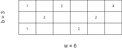
For example Figure 5 indicates the basic functionality in a count min sketch where each item can be hashed into the corresponding slots.
4.2. MDistrib-FIS - Distributed MIDAS using Apache Frequent Item sketch
(anderson2017high) introduces Frequent Item Sketch which belongs to a class of Apache Incubator Datasketches that deals with estimating frequency of items in a streaming environment and is mainly aimed at applications like Heavy-Hitter estimation or estimation of counts of objects in a streaming environment. The Apache Incubator Datasketches framework provide a wrapper api for Frequent Item sketch with the mergeability functionality where two Frequent Item Datasketches and can be merged into one frequent item datasketch with all the frequencies remaining intact .
4.3. : Distributed MIDAS-R
Similar to MDistrib, we take into account the idea of relation attribute used in (bhatia2020midas) for both temporal and spatial relations.
Temporal Relations With the idea of most recent edges being a better representative of the statistic score than previous early edges, for each timestamp id within the partition interval we apply a decay factor where . This is done keeping into consideration the fact that edges from the recent past should compute to the anomaly score calculation as well.
Spatial Relations
As it is also important to capture large group of spatially nearby edges: such as a high out-degree connection from a single source IP address, following MIDAS’s approach we also consider observing nodes with high degree as they occur. For this, we create CMS counters and to approximate the number of edges incident on node at the current time tick and up till respectively. Hence, for a new incoming edge , we compute the anomaly score for edge as well as for node and node and finally take the maximum of the three scores.
4.4. Time complexity Analysis
We focus on time complexity analysis and comparison with respect to MIDAS since MIDAS has performed significantly well in comparison with SOTA models in terms of time complexity.
Considering we have partitions, , where each partition ; belonging to timestamp includes a datasketch. We denote the sketch update time as . If the average number of items during is , then and the total update time for all K partitions under the MIDAS framework would be . Similarly for calculating the sum of the previous edges seen uptil time it can be denoted as where indicates the merge time for two datasketches, Since in both MDistriband MIDASthere is merging of previous current edge sketches, hence remains the same for both.
Comparing the total computation for both the methods, yields
s.t. where denotes the number of total partitions/nodes.
Considering thread allocation time to be very negligible compared to other factors like large number of streaming data points per partition and large number of partitions , it can be seen that is much less than .
Further we also propose reading items per partition to be distributed across various subthreads instead of sequential reading, since each edge under a particular partition/ timestamp can be processed independently of the other. As a result, update time for denoted by can be further reduced to where thus resulting in much faster execution time.
4.5. Better theoretical guarantees
Count Min Sketch Error Estimate
Lemma 4.1.
The error estimate encountered via querying edge counts in MDistrib is less than that of MIDAS by a factor of ()
Proof 1.
MDistribCMS has the same sketch architecture as MIDAS, but however presents with a better theoretical guarantee as shown below:
As per Therrem 1 (cormode2005improved), the estimate from a CMS has the following guarantees: with some probability ,
| (2) |
where the values of these error bounds can be chosen by and , and being the dimensions of the CMS. indicates the total sum of all the counts stored in the data structure. Again considering partitions , let where denote the partition . As per MIDAS the sum sketch for time tick is computed by summation of all previous current edge sketches uptil . Hence for partition , can be written as follows.
For MDistrib-, however since for the partition we have CE sketches, instead of merging them for computing the same, we can individually query each of the sketches instead of merging them. Hence in this case,
Hence, as per Equation. (2) we compare the estimates of the count retrieved from the current Sum CMS sketch of partition for MDistrib and MIDAS.
| (3) |
| (4) |
Since such counts stored in the CMS being non-negative
| (5) |
Hence, taking the inequality from 5 we can conclude that the error bound in the estimate provided by MDistrib is much less than that provided by MIDAS.
| (6) | |||
∎
Apache Frequent Item Sketch Guarantees In case of a Frequent Item Sketch with configuration , where indicates the maximum map size in power of 2 and being the total weights stored in the map, the error in the estimate of the frequency of a particular edge is always bounded within some , , where can be as follows, given is the load factor :
| (7) |
Since Frequent Item Sketch has a similar structure as a Count Min Sketch in terms of the error estimate, the proof for the false positive probability bound also holds here.
Lemma 4.2.
The error estimate encountered via merging two sketches , is the same as that obtained in an original sketch which contains frequencies all items that have been inserted to and as a whole.
Establishing for Count Min Sketch
Considering count min sketches and having dimensions each and inserting an item with actual frequency in both the sketches, then the error estimate of a particular item can be represented as follows
| (8) |
| (9) |
where and indicate the total sum of all the counts stored in CMS and respectively.
By combining Equations. (8) and (9), and since all the elements involved are (), we get the following.
| (10a) | |||
| (10b) | |||
| (10c) | |||
where indicates the total estimated frequency of that particular item, had that item be inserted into the sketch having same dimension which is a combination of and . Hence by this we showcase that the error estimate remains the same even after merging two Count Min Sketches compared to an original Count Min sketch which represents a summation of the two other sketches.
4.6. Why Distributed MIDAS using Apache Frequent Item sketch is better than MIDAS using CMS
Frequent Item Sketch only stores those items at any point that’s larger in freq than the global median frequency, whereas CMS keeps on storing Estimation Errors. Dimitropoulos et al. have introduced the concept of transient keys, which are items that are not active and have low frequency relative to the group, much earlier (dimitropoulos2008eternal).
4.7. Space Complexity
Constant Space for MDistrib-CMS
Considering distributed partitions in our system, at any point we have only current Edge CMS sketches. After the end of partitions, again when we consider the next partitions, in order to store the previous iteration’s sum we maintain another CMS. Hence the total space complexity where and indicate the number of hash functions and buckets in the CMS structure.
Constant Space for MDistrib-FIS
Similarly for Frequent Item Sketch, the total space complexity can be denoted as where is the maximum map size of the data sketch.
4.8. Proofs
Proposition 1 : False Positive Probability Error is more tightly bound in case of MDistrib
Count Min Sketch
As we know for a particular partition , our chi-square statistic can be written as
Theorem 1 (False Positive Probability Bound)
Let be the -quantile of a chi-squared random variable with 1 degree of freedom. Then:
| (11) |
(bhatia2020midas) mentions that the motivation of the above theorem proposal is to show that with a threshold of , as a test statistic results in a false positive probability of at most .
For CMS guarantees 2 we have the following
| (12) |
where is shortened as
We define an adjusted version of our earlier score for the total summation score :
| (13) |
By combining Equations. 11 and 12 by union bound, with probability of at least , we obtain the following.
We denote and as the chi-square test statistic for MIDAS and MDistrib methodologies respectively.
| (14a) | |||
| (14b) | |||
We simplify the equation for MDistrib as it holds the same for MIDAS. From Equation. (13), Equation. (14b) can be simplified as follows.
| (15) | |||
Considering under the assumption that the current edge count is always an estimation of the previous mean plus some positive weight factor,
| (16) | |||
which can be simplified as considering large value of , that is for higher timestamps.
| (17) |
| (18) |
As per Lemma 4.1, we know that
Hence, by combining both the equations, we get
5. Experiments
In this section, we evaluate our proposed anomaly scoring algorithm MDistrib and address to answer the following questions:
- Q1.
Accuracy: How accurately does MDistrib and its variants detect real-world anomalies compared to baselines, as evaluated using the ground truth labels?
- Q2.
Scalability: How does it scale with input stream length? How does the time needed to process each input compare to baseline approaches?
- Q3.
Execution Time: How fast does the proposed method perform with respect to baseline methods while generating anomaly scores in the offline phase?
Baselines: MIDAS-R, SedanSpot, PENnimer, F-Fade
Datasets
In this section, we evaluate performance of MDistrib as compared to other baselines in Table 3 based on 5 real world datasets : DARPA (lippmann1999results) and ISCX-IDS2012 are popular datasets for graph anomaly detection. According to survey [52], there has been proposal of more than 30 datasets and it has been recommended to use CIC-DDoS2019 and CIC-IDS2018 datasets. We also showcase the same for CTU-13 dataset.
| Datasets | |V| | |E| | |T| |
|---|---|---|---|
| DARPA | 25,525 | 4,554,344 | 46,567 |
| ISCX-IDS2012 | 30,917 | 1,097,070 | 165,043 |
| CIC-IDS2018 | 33,176 | 7,948,748 | 38,478 |
| CIC-DDoS2019 | 1,290 | 20,364,525 | 12,224 |
| CTU-13 | 371,100 | 2,521,286 | 33,090 |
Table 2 shows the statistical summary of the datasets. |E| corresponds to the total number of edge records, |V| and |T| are the number of unique nodes and unique timestamps, respectively.
5.0.1. Hyperparameters chosen for baselines
We hereby mention the hyperparameters used by the corresponding baselines.
Spotlight
- •
sample size = 10000
- •
num walk = 50
- •
restart prob = 0.15
MIDAS The size of CMSs is 2 rows by 1024 columns for all the tests. For MIDAS-R, the decay factor = 0.6.
PENimer
- •
ws =1
- •
ms =1
- •
alpha = 1
- •
beta =1
- •
gamma =1
F-Fade
- •
embedding size = 20
- •
= 720
- •
= 120
- •
alpha = 0.999
- •
M =100
For , we always use the timestamp value at the 10th percentile of the dataset.
All methods output an anomaly score corresponding to the incoming edge, a high anomaly score implying more anomalousness. As part of the experiments, we follow the same suite as the baseline papers in reporting the Area under the ROC Curve (using the True Positive Rate TPR and the False Positive Rate FPR) and the corresponding running time. All experiments for calculating the AUC are averaged for 8 runs and the mean is reported along with its spread.
5.1. Experimental Setup
All experiments are carried out on a Intel Core processor, RAM, running OS . We used an open-sourced implementation of MIDAS, provided by the authors, following parameter settings as suggested in the original paper ( hash functions, buckets). We implement MDistrib in python using dask framework. We follow the same parameter settings as MIDAS ( hash functions, buckets).
5.2. Q1. Accuracy
Table 3 includes the AUC of edge anomaly detection baselines along with our two proposed methods and . PENimer is unable to finish in large datasets like CIC-DDos and CIC-IDS within 10 hours range, thus we do not report the result. Among the baseline results and both provide better accuracy results than the baselines on datasets like DARPA, CIC-DDoS and ISCX-IDS.
AUC vs Running Time Figure 6. plots accuracy (AUC) vs. running time (log scale, in seconds) on the Darpa dataset. As we can see both and achieve higher accuracy results than the base lines in considerable less time.

| Methods | DARPA | CIC-DDoS | CIC-IDS | CTU-13 | ISCX-IDS |
|---|---|---|---|---|---|
| -R | 0.953 0.001 | 0.986 0.003 | 0.979 0.01 | 0.908 0.002 | 0.806 0.001 |
| Spotlight | 0.89 0.001 | 0.67 0.002 | 0.42 0.003 | 0.74 0.002 | 0.63 0.001 |
| MIDAS-R | 0.95 0.005 | 0.984 0.003 | 0.96 0.01 | 0.973 0.005 | 0.81 |
| PENimer | 0.87 | - | - | 0.604 | 0.51 |
| F-Fade | 0.91 0.005 | 0.72 0.02 | 0.61 0.03 | 0.802 0.001 | 0.62 0.004 |
| -R | 0.98 0.0004 | 0.986 0.001 | 0.96 0.0005 | 0.92 0.004 | 0.93 0.0001 |
| Methods | DARPA | CIC-DDoS | CIC-IDS | CTU-13 | ISCX-IDS |
|---|---|---|---|---|---|
| -R | 857ms | 971ms | 741ms | 436ms | 3.7s |
| Spotlight | 129.1s | 697.6s | 209.6s | 86s | 19.5s |
| MIDAS-R | 1.4s | 2.2s | 1.1s | 0.8s | 5.3s |
| PENimer | 5.21hrs | 24hrs | 10hrs | 8hrs | 1.3hrs |
| F-Fade | 317.8s | 18.7s | 279.7s | 19.2s | 137.4s |
| -R | 832ms | 962ms | 764.8s | 441ms | 3.1s |
‘
5.3. Q2. Scalability

In Figure 7 we showcase how via distributed processing of individual nodes and computing the sketch results in significant time improvement of execution. We plot the wall clock time needed to run the first number of edges of the DARPA dataset for both MDistrib and MIDAS. At the same time, we showcase that the number of edges increase exponentially, MDistrib shows linearity of increase in execution time similarly as compared to MIDAS for number of partitions = 1463.


5.4. Q3. Execution : GPU based Execution
In addition to our proposed solution, we also extend MDistrib to a GPU setting. For this we created a dask cluster hosted on Saturn cloud11 1 https://saturncloud.io/ and ran our analysis on the same. We use Python’s JupyterLab for running our experiments with server configuration of T4-XLarge, with 4 crores, 16GB of RAM and 1 GPU. In addition we use cuDF22 2 https://docs.rapids.ai/api/cudf/stable/, python’s GPU dataframe library to store our data. We showcase here the experiments done for the DARPA dataset here. Using the above configurations and setting , we achieved an execution time of 672ms which is times faster than MDistrib in non-GPU environment.
As a separate experiment, we increased the number of workers to 10 and achieved execution time of 438ms on DARPA dataset. Further we showcase the GPU utilization and the task status for each of the 10 worker threads. Fig. 9(a) shows the GPU utilization for MDistrib using partitions = 1463 and number of workers = 10.
Figure.8(a) and Figure.10 shows the task status for worker numbers =3 and 10 respectively. Each of the task status depicts the number of underlying processes involved like reading data from a partition and processing it and writing it. Figure 9(b) thus depicts the resources like number of threads or cpu cycles being utilized during the program execution by each of the 10 workers.
6. Conclusion
In this paper, we proposed MDistribwhich uses a distributed strategy to detect anomalous edges in an offline setting. We further showcase that through our distributed sketch architecture, we achieve a better false positive theoretical guarantee and as well as better performance in terms of running time as compared to state of the art methods for large graphs (billion number of edges). We also extend our method to GPU enabled environment to showcase the applicability of our system in high performance computing environments. Lastly we showcased a generalized model of our framework that can use any frequency based sketch and achieve good accuracy results in detecting suspicious anomalies.
References
- [1] Daniel Anderson, Pryce Bevan, Kevin Lang, Edo Liberty, Lee Rhodes, and Justin Thaler. A high-performance algorithm for identifying frequent items in data streams. In Proceedings of the 2017 Internet Measurement Conference, pages 268–282, 2017.
- [2] Siddharth Bhatia, Bryan Hooi, Minji Yoon, Kijung Shin, and Christos Faloutsos. Midas: Microcluster-based detector of anomalies in edge streams. In AAAI 2020 : The Thirty-Fourth AAAI Conference on Artificial Intelligence, 2020.
- [3] Monowar H Bhuyan, Dhruba Kumar Bhattacharyya, and Jugal K Kalita. Network anomaly detection: methods, systems and tools. IEEE Communications Surveys & Tutorials, 16(1):303–336, 2013.
- [4] Varun Chandola, Arindam Banerjee, and Vipin Kumar. Anomaly detection: A survey. ACM computing surveys (CSUR), 41(3):1–58, 2009.
- [5] Yen-Yu Chang, Pan Li, Rok Sosic, MH Afifi, Marco Schweighauser, and Jure Leskovec. F-fade: Frequency factorization for anomaly detection in edge streams. In Proceedings of the 14th ACM International Conference on Web Search and Data Mining, pages 589–597, 2021.
- [6] Graham Cormode and Shan Muthukrishnan. An improved data stream summary: the count-min sketch and its applications. Journal of Algorithms, 55(1):58–75, 2005.
- [7] Xenofontas Dimitropoulos, Marc Stoecklin, Paul Hurley, and Andreas Kind. The eternal sunshine of the sketch data structure. Computer Networks, 52(17):3248–3257, 2008.
- [8] Jeff Donahue, Philipp Krähenbühl, and Trevor Darrell. Adversarial feature learning. arXiv preprint arXiv:1605.09782, 2016.
- [9] Dhivya Eswaran, Christos Faloutsos, Sudipto Guha, and Nina Mishra. Spotlight: Detecting anomalies in streaming graphs. In KDD, 2018.
- [10] Q He, YJ Zheng, CL Zhang, and HY Wang. Mtad-tf: Multivariate time series anomaly detection using the combination of temporal pattern and feature pattern. Complexity, 2020, 2020.
- [11] Richard Lippmann, Robert K Cunningham, David J Fried, Isaac Graf, Kris R Kendall, Seth E Webster, and Marc A Zissman. Results of the darpa 1998 offline intrusion detection evaluation. In Recent advances in intrusion detection, volume 99, pages 829–835, 1999.
- [12] Rui Liu, Siddharth Bhatia, and Bryan Hooi. Isconna: Streaming anomaly detection with frequency and patterns. arXiv preprint arXiv:2104.01632, 2021.
- [13] Murugaraj Odiathevar, Winston KG Seah, and Marcus Frean. A hybrid online offline system for network anomaly detection. In 2019 28th International Conference on Computer Communication and Networks (ICCCN), pages 1–9. IEEE, 2019.
- [14] Guansong Pang, Chunhua Shen, Longbing Cao, and Anton Van Den Hengel. Deep learning for anomaly detection: A review. ACM Computing Surveys (CSUR), 54(2):1–38, 2021.
- [15] Thomas Schlegl, Philipp Seeböck, Sebastian M Waldstein, Georg Langs, and Ursula Schmidt-Erfurth. f-anogan: Fast unsupervised anomaly detection with generative adversarial networks. Medical Image Analysis, 54:30–44, 2019.
- [16] Ya Su, Youjian Zhao, Chenhao Niu, Rong Liu, Wei Sun, and Dan Pei. Robust anomaly detection for multivariate time series through stochastic recurrent neural network. In Proceedings of the 25th ACM SIGKDD International Conference on Knowledge Discovery & Data Mining, pages 2828–2837, 2019.
- [17] Nguyen Thanh Tam, Matthias Weidlich, Bolong Zheng, Hongzhi Yin, Nguyen Quoc Viet Hung, and Bela Stantic. From anomaly detection to rumour detection using data streams of social platforms. Proceedings of the VLDB Endowment, 12(9):1016–1029, 2019.
- [18] Houssam Zenati, Chuan Sheng Foo, Bruno Lecouat, Gaurav Manek, and Vijay Ramaseshan Chandrasekhar. Efficient gan-based anomaly detection. arXiv preprint arXiv:1802.06222, 2018.
- [19] Yu Zheng, Ming Jin, Yixin Liu, Lianhua Chi, Khoa T Phan, and Yi-Ping Phoebe Chen. Generative and contrastive self-supervised learning for graph anomaly detection. IEEE Transactions on Knowledge and Data Engineering, 2021.