Topology optimization of stiff structures under self-weight for given volume using a smooth Heaviside function
P. Kumar 11 1 pkumar@mae.iith.ac.in; prabhatkumar.rns@gmail.com
Department of Mechanical and aerospace Engineering, Indian Institute of Technology Hyderabad, 502285, India
Department of Mechanical Engineering, Indian Institute of Science,
Bengaluru, 560012, Karnataka, India
Published22
2
This pdf is the personal version of an article whose final publication is available at Structural and Multidisciplinary Optimization in Structural and Multidisciplinary Optimization,
DOI:10.1007/s00158-022-03232-x
Submitted on 19 November 2021, Revised on 09 March 2022, Accepted on 14 March 2022
Abstract:
This paper presents a density-based topology optimization approach to design structures under self-weight load. Such loads change their magnitude and/or location as the topology optimization advances and pose several unique challenges, e.g., non-monotonous behavior of compliance objective, parasitic effects of the low-stiffness elements, and unconstrained nature of the problems. The modified SIMP material scheme is employed with the three-field density representation technique (original, filtered, and projected design fields) to achieve optimized solutions close to 0-1. A novel mass density interpolation strategy is proposed using a smooth Heaviside function, which provides a continuous transition between solid and void states of elements and facilitates tuning of the non-monotonous behavior of the objective. A constraint that implicitly imposes a lower bound on the permitted volume is conceptualized using the maximum permitted mass and the current mass of the evolving design. Sensitivities of the objective and self-weight are evaluated using the adjoint-variable method. Compliance of the domain is minimized to achieve the optimized designs using the Method of Moving Asymptotes. The Efficacy and robustness of the presented approach are demonstrated by designing various 2D and 3D structures involving self-weight. The proposed approach maintains the constrained nature of the optimization problems and provides smooth and rapid objective convergence.
Keywords: Topology optimization; Self-weight; Design-dependent loads; Heaviside projection function; Compliance minimization
1 Introduction
Topology optimization (TO) is gaining popularity constantly as a design tool to find optimized material distributions for a wide range of problems, including single- and/or multi-physics concepts (Sigmund and Maute 2013). Problems involving their self-weight loads, design-dependent forces (Kumar et al. 2020), provide various distinctive challenges (Bruyneel and Duysinx 2005), e.g., (1) non-monotonous characteristics of the compliance objective with respect to the design variables, (2) tendency to lose constrained nature of the compliance optimization problems with given volume constraints and (3) the parasitic effects of low-stiffness elements. Note that parasitic effects are also observed in the eigenvalues maximization problem with the Solid Isotropic Material with Penalization (SIMP) (Pedersen 2000). Civil engineering structures typically encounter self-weight loads and thus, their performances are directly associated with the location of optimized material distributions (Bruyneel and Duysinx 2005). In addition, consideration of the self-weight may be essential for designing large-scale structures. Herein, the motif is to present a density-based TO approach covering all the aforementioned challenges to optimize 2D and 3D structures subjected to self-weight. In a typical density-based TO approach, each finite element (FE) is assigned a design variable (material density) that is assumed to be constant within the element. and indicate the solid and void phases of the element, respectively.
Design-dependent loads typically alter their location, magnitude and/or direction as TO progresses and therefore, their sensitivities with respect to the design variables need to be considered within TO formulation (Kumar et al. 2020; Kumar and Langelaar 2021). In such loading scenarios, the overall sensitivities of the compliance objective with respect to the design variables no more remain always negative (see Sec. 3.2) and hence, compliance loses its most cherished monotonic characteristics in a TO setting with self-weight (Bruyneel and Duysinx 2005). In addition, when the effects of self-weight dominate, the optimization problem becomes unconstrained, and the corresponding optimized designs may be nonsensical in the mechanical viewpoint. Further, as per Bruyneel and Duysinx 2005, the parasitic effects are due to low-stiffness elements wherein the ratio between---gravity force to design variables and stiffness to design variables tend to become unbounded. The proposed approach offers a solution to the above-mentioned anomalies while providing optimized solutions close to 0-1 and subduing parasitic effects. A schematic diagram for a 2D structure33 3 2D structure diagram is taken for simplicity. experiencing self-weight (gravity load) and also, an external constant load, F, is depicted in Fig. 1(a). Presence of an external load may not always essential though. A possible solution to the problem (Fig. 1(a)) is displayed in Fig. 1(b). It can be noted that location and magnitude of the gravity load change, which pose challenges in a TO formulation. Next, we review TO approaches presented for designing structures subjected to self-weight.
In a structural optimization framework, self-weight was accounted first by Rozvany 1977. Subsequently, several researchers have presented different TO approaches including self-weight. Bruyneel and Duysinx 2005 identified challenges to include self-weight in continuum-based TO settings. With a linear mass density interpolation, they found that when the design variables attain their lower bounds then the ratio between the mass density (gravity load or self-weight) and the material stiffness obtained by using the classical SIMP formulation tends to infinity. Consequently, displacements become unbounded and that in turn makes compliance unbounded. As per them, the optimizer tries to avoid unboundedness of the displacement field by providing design variables in , i.e. gray elements. To subdue such unrealistic gray material, they altered the SIMP formulation using a threshold density value and regarded material stiffness linear below , which introduces non-differentiability in the material model. This paper however shows that with the modified SIMP formulation (Sigmund 2007), a smooth material (stiffness) interpolation scheme, in conjunction with the three-field density technique (Lazarov et al. 2016), one can circumvent parasitic effects.
Ansola et al. 2006 proposed a modified evolutionary structure optimization approach to design structures under self-weight. They presented a correction factor to compute the sensitivities of the objective and to enhance the convergence of the optimization. Huang and Xie 2011 used the bi-directional evolutionary structural optimization approach with the RAMP material model (Stolpe and Svanberg 2001) for designing structures subjected to self-weight. Xu et al. 2013 proposed the guide-weight approach using the optimality criteria method. They employed the SIMP and the RAMP material models to demonstrate their approach. Chang and Chen 2014 presented a modified gradient projection method to solve problems involving density-dependent forces. Holmberg et al. 2015 employed the non-linear semi-definite programming for the worst-case TO with self-weight. A closed B-splines-based approach was proposed by Zhang et al. 2017 to avoid parasitic effects of low-density regions for design-dependent loads. Félix et al. 2020 employed a power-law function for the material density interpolation to reduce the parasitic effects. Fernandez et al. 2020 presented a design optimization approach using the three-filed technique for simultaneously optimizing material, shape and topology. They used level-set functions to implicitly represent the boundaries and considered design-dependent pressure (Kumar et al. 2020) and self-weight loads. Novotny et al. 2021 proposed a topological derivative-based TO approach using a regularized formulation for imposing feasible volume constraints for structures under self-weight.
This paper presents an approach using the standard density-based TO with the modified SIMP scheme (Sigmund 2007) in conjunction with the three-field density representation technique (original, filtered and projected design fields, cf. Lazarov et al. 2016) for the design problems involving self-weight. The parameter associated with the three-field technique is updated using a continuation scheme to achieve optimized designs close to 0-1. A novel mass density interpolation strategy is presented using a smooth Heaviside function. This interpolation scheme provides a continuous transition between the void and solid states of the element and controls the non-monotonous behavior of the objective. A constraint is formulated using the maximum permitted self-weight (proportional to the given volume fraction) and the current self-weight of the evolving design. This constraint implicitly imposes a lower bound on the permitted volume. Consequently, the tendency to lose constrained nature of the problem is subdued. Load sensitivities are evaluated using the computationally cheap adjoint-variable method. Compliance is minimized to obtain optimized material layouts for various structures subjected to self-weight with different boundary specifications. We use the Method of Moving Asymptotes (Svanberg 1987) to solve the formulated optimization problem. The approach can be readily extended for three-dimensional problems, which is demonstrated by solving two 3D numerical examples.
In summary, this paper offers the following new aspects:
- •
A density-based topology optimization approach using the three-field (original, filtered and projected) representation technique in conjunction with the modified SIMP scheme to design stiff structures subjected to self-weight.
- •
Formulation of a novel mass density interpolation strategy using a smooth Heaviside function. The interpolation helps tune/control the non-monotonous behavior of the objective by using suitable mass density parameters (Sec. 2).
- •
Conceptualization of a new constraint within the optimization formulation that implicitly provides a lower bound on the permitted volume fraction for the given problem. When the effects of self-weight dominate, this constraint is necessary to retain the constrained nature of the problem (Sec. 3).
- •
Demonstration of the efficacy and robustness of the presented approach by designing various structures subjected to self-weight. Optimized solutions are close to 0-1 with smooth objective and constraints convergence, and thus parasitic effects are subdued (Sec. 4).
- •
Extension of the approach for 3D topology optimization design problems including self-weight (Sec. 4).
The layout of this paper is structured as follows. Section 2 describes the modeling of self-weight and the proposed mass density interpolation scheme. Problem description including the topology optimization formulation and sensitivity analysis is presented in Section 3. Next, numerical examples for various 2D and 3D design problems involving self-weight are presented in Section 4. Pertinent discussions and a study with different parameters are also presented. Section 4.3 demonstrates three-dimensional results. Lastly, conclusions are drawn in Section 5.
2 Self-weight modeling
Self-weight arises due to the gravitational acceleration , which acts vertically downward. In a continuum setting, can be determined as
| (1) |
where () is mass density of the material used, () represents volume of the domain, and , where g and , a unit vector, directs in positive and directions for 2D and 3D settings respectively.
In a discrete setting, the elemental self-weight is evaluated as (Cook et al. 2007)
| (2) |
where . is the identity matrix in , indicates dimension of the domain. and for 2D and 3D cases, respectively. is the mass density of element . Nno is the total number of nodes per element employed to discretize the design domain. We use four-noded quadrilateral and eight-noded hexahedral finite elements (FEs) to describe the two- and three-dimensional design domains respectively, i.e, Nno (for 2D) and Nno (for 3D).
In a typical TO framework, each finite element displays solid () and void ( ) material phases; denotes the physical design variable of element (see Sec. 3). Herein, the mass density of each FE is related to . Elements with and have (mass density of void FE) and (mass density of solid FE) mass density respectively. A smooth Heaviside function is employed to evaluate the mass density of each FE using its both states that offers continuous transition between the phases of the element as TO progresses. In addition, the proposed interpolation scheme not only provides the load sensitivities readily (see Sec. 3.2), it offers a way to tune the non-monotonous behavior of the objective using the proper mass density parameters (3) as described below. Mathematically, the mass density interpolation is written as
| (3) |
where is used; is termed the mass density contrast. The smooth Heaviside projection function is defined using the physical design variables as (Wang et al. 2011)
| (4) |
where both and are adjustable parameters that provide the position of step and the slope. and are called the mass density parameters herein. Fig. 2 depicts mass density interpolation function for different and . For higher more sharpness i.e. sharp transition from the void state to solid phase can be noted (Fig. 2).
In view of shape functions of quadrilateral (2D) and hexahedral (3D) elements in association with the Gauss-quadrature points, (2) in light of (3) gives (Cook et al. 2007)
| (5) |
where and
for 2D and 3D settings respectively, and (for 2D), (for 3D). , , and represent the length, width, height and thickness of the design domain. The derivatives of gravity force with respect to can be readily evaluated as
| (6) |
where
Finally, the elemental forces are assembled to determine the total (global) gravity load experienced by the design in a discrete setting and thus, compliance of the domain and are evaluated.
As per (6), , i.e., is a function of physical design variable at desirable and thus, alters as TO progresses. This is expected to help the exploratory characteristics of the TO process (Kumar et al. 2020). Fig. 3 depicts different plots of with respect to , where is the component of , at the same sets of those are used in Fig. 2. determines the location of the peak of the derivative curve on -axis whereas, controls the sharpness of the curve at (Fig. 3). Elements with design variables lower than have mass density close to (Fig. 2). A higher can give a relatively sharper peak at and thus, it can jeopardize the TO process. Therefore, for a given design problem, is selected so that used initial guess for the design vector, typically taken equal to the given volume fraction, remains at a proper distance from towards the right side on -axis wherein the derivatives of are relatively much lower (Fig. 3). In this way, the non-monotonous behavior of the objective can be tuned for the given problem. Consequently, the optimization process becomes smooth and gives mechanical sensible designs (see Sec. 4). We provide a recommendation to decide for a given design problem in Sec. 4.2.2 based on the numerical experiments performed therein. Next, the problem formulation is presented.
3 Problem formulation
The density-based topology optimization in conjunction with the three-field density formulation (Lazarov et al. 2016) is used in the presented approach. For the Young’s modulus interpolation, the modified SIMP formulation (Sigmund 2007) is employed that relates modulus of elasticity of element to its physical design variable using the power law as
| (7) |
where and are Young’s moduli of the void and the solid phases of element , respectively. The material contrast, i.e. is set and , the SIMP penalty parameter, is set to 3 that guides TO convergence towards ‘0-1’ designs.
In the three-field () density representation technique (Lazarov et al. 2016), , and denote vectors containing the original design variables , filtered design variables and physical design variables respectively. The chain of transformation between these variables can be denoted via (Lazarov et al. 2016).
The filtered variables , determined using a mesh-independent density filtering scheme (Bruns and Tortorelli 2001), is given as
| (8) |
where indicates the total number of neighboring elements of element , is the volume of the element . , the weight function, is determined using the Euclidean distance between the centroids and of elements and as
| (9) |
where is the employed filter radius. One can write (8) in the matrix form as
| (10) |
where represents the set of neighboring elements for element within the given filter radius . We compute filter matrix once in the beginning of the algorithm, store it as a sparse matrix and use it within the optimization loop to evaluate the filtered design vector . The derivatives of with respect to is calculated as
| (11) |
The physical design variable , determined using corresponding filtered variable and a smooth Heaviside function which is analogous to (4), is given as
| (12) |
where controls the sharpness of the Heaviside function . Typically is increased in a continuation fashion from its initial value to maximum value to achieve the solution close to 0-1 (Wang et al. 2011). In turn, parasitic effects of the low-density element can be suppressed. Herein, is set, and is doubled after every 25 optimization iterations. With and , one achieves the minimum length scale on the void and solid phase respectively (Wang et al. 2011), and also, attains the Heaviside approximation given by Guest et al. 2004 and Sigmund 2007 respectively. One determines the derivative of with respect to as
| (13) |
Using the chain rule, the derivative of a function with respect to the actual design variable can be determined in view of (11) and (13) as
| (14) |
wherein can be determined for the given objective function (see Sec. 3.2).
3.1 Topology optimization formulation
The compliance (strain energy) of the structures subject to self-weight and/or external constant load is minimized to obtain the optimized topologies. The optimization problem is formulated as
| (15) |
where represents the objective function, i.e., compliance of the structure, and are the global force vectors arise due to the self-weight and external loads respectively, and indicates the strain energy. is a user defined scalar quantity. and are the global stiffness matrix and the displacement vector respectively. and are constraints. and are the design volume and permitted volume respectively. , where is the permitted volume fraction. (vector), (scalar) and (scalar) are the Lagrange multipliers corresponding to the state equations, g1 and g2 respectively.
Herein, constraint g2 is applied such that a lower bound on the volume fraction can implicitly be realized. It is formulated using the maximum permitted mass determined using the given volume fraction, , and the intermediate mass of the evolving design, wherein indicates mass of element e. Sec. 4.1 and Sec. 4.1.3 substantiate the requirement of this constraint for a given volume when the effects of self-weigh dominate via numerical examples. This constraint helps retain the constrained nature of the problem. For the finite element analysis, the small elastic deformation is assumed herein.
3.2 Sensitivity analysis
A gradient-based optimization technique, the Method of Moving Asymptotes (MMA, cf. Svanberg 1987), is employed to solve the optimization problem mentioned in (15). Thus, derivatives of the objective and constraints with respect to the design variables are required. The derivatives of objective are determined via the adjoint-variable approach. For that, the augmented response is defined using the objective and the state equations as
| (16) |
where is the Lagrange multiplier vector. We henceforth for brevity omit the arguments from the vector and the matrix quantities. Differentiation of (16) with respect to yields
is selected such that 44 4 This is the adjoint equation corresponding to the state equation (15). that yields, and thus, with and at the equilibrium state, one writes
| (17) |
In (17), self-weight sensitivities, appear and they are evaluated using (6). Next, the chain rule (14) is employed to evaluate the objective sensitivities with respect to the design vector, i.e., . Finding sensitivity of constraint g1 is straightforward (Sigmund 2007), whereas that of constraint g2 can be evaluated using (6). Moreover, it can be noted that compliance objective sensitivities can either be negative or positive (17), i.e., they alter their sign as per the different design variables. This shows the non-monotonous behavior of compliance when self-weight is considered. This behavior is controlled herein by the proposed mass density interpolation scheme. The selected (Sec. 4.2.2) mass density interpolation parameters controls (Fig. 3) of , and thus, the non-monotonous behavior. Note that when self-weight effects dominate, always gives positive quantities. Sec. 4.2.2 provides a recommendation for choosing for the given optimization problem based on the numerical examples solved therein. Next, we solve various structure problems subjected to self-weight and provide pertinent discussions.
4 Numerical Examples and Discussions
Herein, the efficacy and robustness of the proposed method are demonstrated by optimizing various structures with self-weight and/or constant external loads. Both 2D and 3D designs are considered. The design domains with boundary conditions are displayed in their respective section. , and are used to indicate length in , and directions respectively. Thickness of the domain is represented by which is set to for the presented 2D design problems. We use bilinear quadrilateral finite elements to describe the 2D design domains, whereas 3D domains are represented via hexahedral FEs. , and denote the total number of FEs employed in , and directions respectively to parameterize the design domain. One can also use honeycomb tessellation (Kumar 2022) to describe the design domain for 2D problems. A density-based TO approach is employed wherein each element is assigned one design variable which is considered constant within the element. TO process is initialized using the given volume fraction. The Youngs’ modulus and mass density of the material are set to and respectively (Xu et al. 2013). The total number of the MMA iterations is set to 250 unless otherwise stated. As mentioned earlier, (12) is doubled after every 25 MMA iterations until it reaches its maximum value 256 and thereafter, it remains so for further iterations. We display the optimized material layouts of the solved numerical examples using their physical design vector (Sigmund 2007). Note that design problems with self-weight have non-convex nature (Bruyneel and Duysinx 2005) and thus, we can neither ensure convergence to the global optimum nor avoid dependence of final solutions on the starting guesses.


4.1 2D design problems
We first present various 2D design-problems experiencing self-weight herein.
4.1.1 Self-weight loadbearing arch geometry
The design domain for the self-weight loadbearing arch structure is depicted in Fig. 4(a). Both ends of the bottom edge are fixed (Fig. 4(a)), and no external force is applied (i.e ). and are taken. The external move limit of the optimizer is set to 0.1. Filter radius is set to . The mass density parameters and are used (4). The permitted volume fraction is set to 0.25.
Qualifying constraint
Problems exclusively with self-weight (when self-weight effects dominate) under a volume constraint lose their constrained nature (Bruyneel and Duysinx 2005). To prevent this tendency, additional constraint g2 which implicitly ensures a lower bound on the resource volume is considered in conjunction with the presented mass density interpolation scheme (3) and the three-field representation technique (Lazarov et al. 2016). The constraint is qualified and substantiated its importance by optimizing the arch design (Fig. 4(a)) with self-weight (15) using different cases and also, by optimizing the MBB beam design in the next section.
To parameterize the design domain, (i) FEs and (ii) FEs are used. This is done to record the behavior of the approach with respect to different mesh sizes. In addition, though the problem is symmetric, the full model is considered to note any tendency to lose the symmetry in the optimized designs. Four cases namely, (i) CASE I: FEs without constraint g2, (ii) CASE II: FEs with constraint g2, (iii) CASE III: FEs without constraint g2, and (iv) CASE IV: FEs with constraint g2 are considered.


The optimized results for all the cases are displayed after 250 MMA iterations in Fig. 5. When constraint g2 is not taken into account, for example in CASE I and CASE III, the optimization problem becomes unconstrained as evident from their volume constraint convergence plots (see Fig. 6(a) and Fig. 6(b)). The optimized design of CASE I contains gray elements (marked in red circles in Fig. 5(a)). On the other hand, with constraint g2 (CASE II and CASE IV) the optimization problem retains its constrained nature and at the end of TO, volume constraint g1 stays active (Fig. 6(a) and Fig. 6(b)). Steps in volume fraction convergence curves are due to updation scheme (12) which is performed to achieve 0-1 optimized solutions. Constraints’ convergence plots for CASE II and CASE IV are displayed in Fig. 7(a) and Fig. 7(b) respectively. Constraints are active at the end of optimization. The optimized designs of CASE II (Fig. 5(b)) and CASE IV (Fig. 5(d)) are close to 0-1 solutions. Topologies of these solutions resemble those reported in (Bruyneel and Duysinx 2005; Huang and Xie 2011; Novotny et al. 2021). Furthermore, these solutions (Fig. 5(b) and Fig. 5(d)) are symmetric with respect to the central axis of the domain and thus, symmetry nature of the problem is retained. We henceforth report convergence history for constraint g1 only in view of Fig. 7.


4.1.2 Arch structure
The design domain (Fig. 4(a)) is described using FEs. The volume fraction is set to 0.40. The external move limit of the MMA is set to 0.05 herein and used henceforth. and are considered. Filter radius is set to . Constraint g2 is considered within the optimization formulation. Other design parameters are same as those employed in Sec. 4.1.1.
The optimized result is depicted in Fig. 8(a), and the corresponding convergence curves for the volume fraction the objective are displayed in Fig. 8(b) and Fig. 9 respectively. The design evolution at different intermediate stages are also shown in Fig. 9. The objective convergence is smooth and relatively rapid. This implies that no unbounded displacements exist and thus, parasitic effects of the low-stiffness elements are circumvented. As increases, the boundaries of the solution become crisp, and the solution moves towards 0-1 design (Fig. 9). The volume constraint is active and satisfied at the end of optimization and thus, constrained nature of the problem is maintained. As (12) is updated at every 25 MMA iterations, corresponding steps in volume fraction can be noted (Fig. 8(b)).


4.1.3 MBB beam design
A Messerschmitt-Bolkow-Blohm (MBB) beam design subjected to self-weight as well as an external load is studied in this example.
In view of symmetric nature of the problem, the right symmetric part (Fig. 4(b)) with dimension and is considered. Magnitude of the external load, applied as shown in Fig. 4(b) in the negative direction, is set to . Different is taken herein. The boundary conditions of the problem are as depicted in Fig. 4(b). The domain is parameterized using FEs. The filter radius is set to . Other parameters are same as those used in Sec. 4.1.1. In this study, three cases are considered.
First, the beam is optimized with , i.e, only self-weight and with different volume fractions, e.g., . The problem is solved with constraint g2. The optimized results are displayed in Figs. 10(a)-10(c), which are very close to 0-1 with similar topologies. Each optimized design has a horizontal bar-typed slender member which is expected with such boundary conditions. As volume fraction increases more material get accumulated near the support in the optimized structures (Figs. 10(a)-10(c)). This occurs to reduce the bending moment of self-weight of the material placed by the optimizer. Convergence curves of the objectives and the volume fractions are depicted in Fig. 11(a) and Fig. 11(b) respectively. The objective convergence is smooth and rapid (Fig. 11(a)) that is also noted previously. Parasitic effects of the low-stiffness elements/regions are not observed. Constrained nature of the problem is preserved as the respective volume constraint is active at the end of optimization (Fig. 11(b)). Moreover, the trends of volume fraction convergence plots are similar as the employed continuation is same for them. The steps in volume convergence curves (Fig. 11(b)) are associated with updation. Figure 12 displays the material layout plots of original (Fig. 12(a)), filtered (Fig. 12(b)) and physical (Fig. 12(c)) fields of the optimized result shown in Fig. 10(a). Fig. 12(a), Fig. 12(b) and Fig. 12(c) have similar typologies. Gray elements can be noted in Fig. 12(a) and Fig. 12(b), however the result in Fig. 12(c) (Fig. 10(a)) is close to 0-1.

Second, we solve the MBB beam design with different magnitudes of F, i.e., with different and constraint g2. The desired resource volume is set to . Other parameters are same as above. The optimized results are shown in Fig. 13. One can note that as decreases, the material gets transferred from the center region to the lateral sides of the domain so that the optimized designs experience less bending moment due to the self-weight. The central structures which support the external load disappear eventually as magnitude of F decreases. The geometry of the optimized layout gradually changes to two connected arch structures facing towards each other. The final compliance decreases as decreases that is as expected. The convergence of objective is found to be smooth and rapid. The volume fractions are satisfied and remain active for all .

Third, the MBB beam design problem is solved without constraint g2 for different (Fig. 14). The corresponding optimized results are displayed in Fig. 14. We note that for (Figs. 14(b)-14(h)) the volume constraint of the problem is although satisfied, is not active at the end of optimization, i.e, the constrained nature of the problem is not retained. On the other hand, the final material volume with is 0.25, i.e., the volume constraint remains active at the end of optimization. Therefore, mere presence of an external load with self-weight for a design problem cannot help retain the constrained nature of the problem unless the magnitude of the applied external load is relatively large (Fig. 14(a)) or a lower bound on the permitted material volume is employed (implicitly/explicitly) (Fig. 13). In other words, as long as the effects of self-weight are prominent in the optimization process, we need constraint like g2 within the optimization formulation to retain the constrained nature of the problem. We henceforth solve all problems with constraint g2.
4.1.4 Tower design
For this example, a design domain for tower structure is considered with self-weight and an external load.
The design domain is displayed in Fig. 15(a). Both ends of the bottom edge are fixed. is taken. Filter radius is equal to . In light of the vertical symmetry, only a symmetric half design domain is consider for simulation and optimization. FEs are employed to parameterize the symmetric half domain. Volume fraction is set to 0.25. Magnitude of the external load is taken equal to the self-weight. The load is applied at the center of the top edge of domain in the negative direction. Other design parameters are same as above.
The optimized tower structure is shown in Fig. 15(b). The objective and the volume fraction convergence plots are displayed in Fig. 15(c). A rapid and smooth convergence for the objective can be noted. The parasitic effects of the low-stiffness regions do not exist. The volume fraction is satisfied and remains active at the end of optimization. The optimized structure is close to 0-1. A vertical slender structure appears in the optimized design (Fig. 15(b)) to contain the applied external load. By and large, the optimized design resembles a typical tower design.


4.1.5 House arch design
In this example, the presented approach is demonstrated by designing a structure resembling a typical house arch structure.
The design domain and boundary conditions are shown in Fig. 16(a) wherein . A non-design void region of size (Fig. 16(a)) is present in the design domain to facilitate entry and exit. The structure is considered under self-weight only, i.e., . Though a vertical symmetry exists, we take full domain to analyze and optimize so that any deviation from symmetry can be noted in presence of a non-design domain. The domain is parameterized by FEs. The permitted volume fraction is 0.40. Filter radius is set to . Other parameters are same as those used above.
The optimized result is displayed in Fig. 16(b). The optimized design is constituted via two pillars and an arch structure on the top. The corresponding convergence plots are depicted in Fig. 16(c). As noted earlier here too the objective convergence is rapid and smooth. One can note that the volume constraint is active at the end of optimization (Fig. 16(c)). The steps in volume fraction convergence curve are due to updation. This indicates that method works well when non-design domains are present.


4.2 Parameter study
In this section, we present the effects of different parameters on the optimized designs with self-weight.
4.2.1 Volume fraction
Herein, different volume fractions ranging from 0.1 to 0.9 are used to solve the arch structure (Fig. 4(a)). FEs is used to represent the design domain. and are considered. Filter radius is set to . Other design parameters are same as those used in Sec. 4.1.1.
Fig. 17 displays a Pareto curve between compliance and volume fractions. As volume fraction increases, self-weight of the optimized design increases and thus, corresponding compliance increases. The optimized results are shown in Fig. 17 for every volume fraction. It is noted that the volume constraint for each case remains active at the end of optimization, and the corresponding objective convergence is rapid and smooth. The optimized design with volume fraction 0.1 is disconnected, which is constituted via two pillars (see Sec. 4.2.2). Compliance with is obtained higher than that with .
4.2.2 Mass density parameters
This study demonstrates the effects of different mass density parameters on the optimized designs with self-weight.
The design domain for this study is shown in Fig. 4(a). Volume fraction is set, and filter radius is taken equal to . FEs is employed to describe the design domain. Note that, controls the slope of material density interpolation (Fig. 2). For higher , elements with act as solid FEs.
The optimized designs with various are depicted in Fig. 18. Topologies of the optimized designs are similar in Fig. 18(b) and Fig. 18(c) but having different final objective values. The obtained final objective value with is lower than those of all other cases considered, which suggests and confirms that indeed an arch-shaped structure is the actual optimized design for the problem shown in Fig. 4(a). Optimized designs shown in Fig. 18(a), Fig. 18(d) are disconnected, and their final compliance are higher than the other two in Fig. 18. The optimized design displays in Fig. 18(b) is asymmetric (central region). A possible reason may be the numerical noise during optimization. Note however that with a suitable choice of , one can also retain symmetric nature of the problems in their optimized designs (Fig. 18(c)) as progress of the optimization process is relatively stable i.e less noisy due to lower non-monotonous behavior of the objective. For the tuning the latter, should be sufficiently far and towards left on design variable axis from the given volume fraction (Fig. 2). When decreasing and increasing , the region of transitions from void to solid reduces (Fig. 2) and in those cases, the optimized designs are found to be connected and sensible. Relatively moderate and offers smoother optimization problem, however the final obtained designs may be disconnected. Thus, in general, and can be chosen such that a suitable trade-off between the differentiability and transition i.e a suitable span of transition from void to solid phases for the given problem can be obtained (Fig. 2) and also, non-monotonous behavior of the objective is reduced (Fig. 3). By and large, based on our experience, less than and equal to and between ensure the desired trade-off. To demonstrate that indeed the recommended values work, we solve the problem for permitted volume fractions 0.1, 0.15, 0.5 and 0.6 with as their . Fig. 19 shows the optimized design. These designs are connected and sensible. We also notice that choosing and work fine, for all the cases reported with the respective , which simplifies while retaining the novelties of the proposed mass density interpolation scheme (3) to or . In addition, the volume constraints for all cases are found to be satisfied and active at the end of optimization.




4.3 Three-dimensional examples
This section demonstrates that the proposed approach can without much difficulty be extended for 3D problems including self-weight. TO is performed using an in-house MATLAB code wherein the conjugate gradient method in association with incomplete Cholesky preconditioning is employed to solve the linear systems from the equilibrium and adjoint equations.
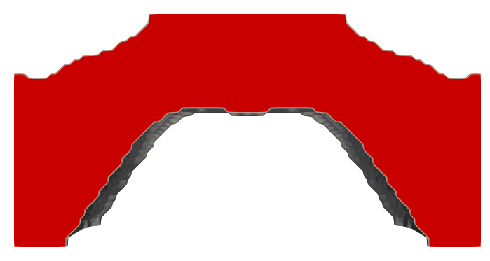
Two 3D problems are solved: (i) an arch structure problem with only self-weight and (ii) a tower structure with self-weight and a central constant load. Their design domains are displayed in Fig. 20. For the arch structure, we exploit one symmetry axis for the analysis and optimization (Fig. 20(a)), whereas for the tower problem both symmetry axes are exploited (Fig. 20(b)). The symmetric parts used for optimization are shadowed using light cyan color (Fig. 20).
and are considered for the arch design (Fig. 20(a)) and the tower design (Fig. 20(b)) respectively. The half symmetric part of arch domain (colored shape in Fig. 20(a)) is parameterized via hexahedral FEs, whereas the quarter part of the tower domain (colored shape in Fig. 20(b)) is described via FEs. The permitted volume fractions, filter radii and material density parameters for arch and tower design problems are set to 0.35 and 0.1, and , and and respectively. Other design parameters are the same as those used in the above sections.
Figure 21 and Fig. 22 show the optimized arch and tower designs in different view directions respectively. An isosurface with the physical density value at 0.90 is taken to plot the optimized results. The results in an isoview direction are displayed in Fig. 21(a) and Fig. 22(a) respectively. It can be noted that direction view of the optimized 3D arch result (Fig. 21(c)) resembles that obtained for the 2D arch structure (Fig. 8(a)). For both designs, the optimizer has succeeded in providing the optimized shape which can be more advantageous for the compliance objective. The material distribution pertaining to different cross-sections for the arch and tower structures are shown in Fig. 23(a) and Fig. 23(b) respectively. It can be noticed that the material distributions at the cross-sectional areas are close to 1.0 indicating that the optimized results are closed to binary. In addition, the results render clear design interpretation. We can expect relatively more detailed features in the optimized tower design with much finer mesh which can be efficiently obtained using fully parallelized framework, which forms one of the future works.
5 Closure
This paper presents a novel density-based topology optimization approach to optimize continua involving self-weight. The robustness and versatility of the approach are demonstrated by optimizing various 2D and 3D structures subjected to self-weight. The compliance of the structure is minimized using the Method of Moving Asymptotes with a given volume constraint and a conceptualized constraint.
When the effects of self-weight dominate, the optimization problem tends to become unconstrained. We conceptualize a constraint using the maximum permitted mass and intermediate mass of the design domain that implicitly imposes the lower bound on the given volume fraction. With this constraint, the given volume fraction for the problem gets satisfied and remains active at the end of the optimization, i.e., the constrained nature of the problem is retained. With self-weight, the optimized results are significantly different and thus, it should not be neglected in design problems wherein effects of self-weight prevail. The mass density of each element is proposed to interpolate using a smooth Heaviside projection function that offers continuous transition between the phases of elements as topology optimization advances. Using the proper mass density parameters, the non-monotonous behavior of the objective is tuned/controlled. The mass density parameters are selected a priori to the optimization that affect the optimized topologies. The recommended range of values for them are provided based on the numerical examples solved.
The modified SIMP material interpolation method is employed in conjunction with a three-field density representation technique. Parameter is increased using a continuation scheme such that the optimized designs can be steered toward close to 0-1 solutions. The presented approach works well with designs containing non-design domains, which is demonstrated via a house arch design containing a non-design void region. The approach maintains symmetric nature of problem in the optimized structures. The approach is easily extended to 3D problem settings that is demonstrated by solving two three-dimensional problems (a 3D arch structure experiencing only self-weight and a 3D tower structure experiencing both self-weight and external load). It is noted that convergence of the objective is smooth and rapid while obtaining the solutions close to 0-1, i.e. the parasitic effects are subdued. The optimized results provide clear design interpretation. Design problems with self-weight have non-convex nature and therefore, convergence to the global optimum and dependence of the optimized solutions on the starting guesses cannot be ensured. Extending the approach with advanced constraints, e.g., stress constraint, bucking constraint forms future research directions.
Acknowledgment
The author would like to thank Professor G. K. Ananthasuresh for fruitful discussions, Professor Krister Svanberg for providing MATLAB codes of the MMA optimizer and acknowledge financial support from the Science & Engineering research board, Department of Science and Technology, Government of India under the project file number RJF/2020/000023.
References
- Ansola et al. (2006) Ansola R, Canales J, Tarrago JA (2006) An efficient sensitivity computation strategy for the evolutionary structural optimization (eso) of continuum structures subjected to self-weight loads. Finite elements in analysis and design 42(14-15):1220–1230
- Bruns and Tortorelli (2001) Bruns TE, Tortorelli DA (2001) Topology optimization of non-linear elastic structures and compliant mechanisms. Computer methods in applied mechanics and engineering 190(26-27):3443–3459
- Bruyneel and Duysinx (2005) Bruyneel M, Duysinx P (2005) Note on topology optimization of continuum structures including self-weight. Structural and Multidisciplinary Optimization 29(4):245–256
- Chang and Chen (2014) Chang C, Chen A (2014) The gradient projection method for structural topology optimization including density-dependent force. Structural and Multidisciplinary Optimization 50(4):645–657
- Cook et al. (2007) Cook RD, Malkus DS, Plesha ME, Witt RJ (2007) Concepts and applications of finite element analysis. John wiley & sons
- Félix et al. (2020) Félix L, Gomes AA, Suleman A (2020) Topology optimization of the internal structure of an aircraft wing subjected to self-weight load. Engineering Optimization 52(7):1119–1135
- Fernandez et al. (2020) Fernandez F, Barker AT, Kudo J, Lewicki JP, Swartz K, Tortorelli DA, Watts S, White DA, Wong J (2020) Simultaneous material, shape and topology optimization. Computer Methods in Applied Mechanics and Engineering 371:113321
- Guest et al. (2004) Guest JK, Prévost JH, Belytschko T (2004) Achieving minimum length scale in topology optimization using nodal design variables and projection functions. International journal for numerical methods in engineering 61(2):238–254
- Holmberg et al. (2015) Holmberg E, Thore CJ, Klarbring A (2015) Worst-case topology optimization of self-weight loaded structures using semi-definite programming. Structural and Multidisciplinary Optimization 52(5):915–928
- Huang and Xie (2011) Huang X, Xie Y (2011) Evolutionary topology optimization of continuum structures including design-dependent self-weight loads. Finite Elements in Analysis and Design 47(8):942–948
- Kumar (2022) Kumar P (2022) HoneyTop90: A 90-line MATLAB code for topology optimization using honeycomb tessellation. Optimization and Engineering
- Kumar and Langelaar (2021) Kumar P, Langelaar M (2021) On topology optimization of design-dependent pressure-loaded three-dimensional structures and compliant mechanisms. International Journal for Numerical Methods in Engineering 122(9):2205–2220
- Kumar et al. (2020) Kumar P, Frouws J, Langelaar M (2020) Topology optimization of fluidic pressure-loaded structures and compliant mechanisms using the darcy method. Structural and Multidisciplinary Optimization 61(4)
- Lazarov et al. (2016) Lazarov BS, Wang F, Sigmund O (2016) Length scale and manufacturability in density-based topology optimization. Archive of Applied Mechanics 86(1-2):189–218
- Novotny et al. (2021) Novotny A, Lopes C, Santos R (2021) Topological derivative-based topology optimization of structures subject to self-weight loading. Structural and Multidisciplinary Optimization 63(4):1853–1861
- Pedersen (2000) Pedersen NL (2000) Maximization of eigenvalues using topology optimization. Structural and multidisciplinary optimization 20(1):2–11
- Rozvany (1977) Rozvany GI (1977) Optimal plastic design: allowance for self-weight. Journal of the Engineering Mechanics Division 103(6):1165–1170
- Sigmund (2007) Sigmund O (2007) Morphology-based black and white filters for topology optimization. Structural and Multidisciplinary Optimization 33(4-5):401–424
- Sigmund and Maute (2013) Sigmund O, Maute K (2013) Topology optimization approaches. Structural and Multidisciplinary Optimization 48(6):1031–1055
- Stolpe and Svanberg (2001) Stolpe M, Svanberg K (2001) An alternative interpolation scheme for minimum compliance topology optimization. Structural and Multidisciplinary Optimization 22(2):116–124
- Svanberg (1987) Svanberg K (1987) The method of moving asymptotes–a new method for structural optimization. International journal for numerical methods in engineering 24(2):359–373
- Wang et al. (2011) Wang F, Lazarov BS, Sigmund O (2011) On projection methods, convergence and robust formulations in topology optimization. Structural and Multidisciplinary Optimization 43(6):767–784
- Xu et al. (2013) Xu H, Guan L, Chen X, Wang L (2013) Guide-weight method for topology optimization of continuum structures including body forces. Finite Elements in Analysis and Design 75:38–49
- Zhang et al. (2017) Zhang W, Zhao L, Gao T (2017) Cbs-based topology optimization including design-dependent body loads. Computer Methods in Applied Mechanics and Engineering 322:1–22