Perturbing Isoradial Triangulations
Abstract.
We consider infinite, planar, Delaunay graphs obtained by locally deforming the coordinate embedding of a general, isoradial graph , with respect to a real deformation parameter . We study three operators on : the Beltrami-Laplace operator , a conformal Laplacian , and the David-Eynard Kähler operator . The determinant of the later appears is the model of random Delaunay triangulations proposed by [DE14], where it was conjectured to be a discrete version of the Faddeev-Popov determinant in Polyakov’s theory of 2D gravity (Liouville gravity).
All three operators coincide in the limit with R. Kenyon’s critical Laplacian on , whose Green’s function is known. Using Kenyon’s exact and asymptotic results for we calculate the first and second order terms in the -expansion of the log-determinant of , and , and then study the large distance asymptotics of the bi-local part in the second order term. This entails a careful analysis of edge flips induced by the deformation and the Delaunay constraints.
We show that scaling limits of the second order bi-local term for both and exist and are independent of the choice of initial isoradial graph , while such a scaling limit does not exist in general for (due to the formation of curvature dipoles). Moreover we find that the scaling limits for and coincide.
We define a discrete analogue of the stress-energy tensor for each of the three operators, and interpret the scaling limits of the bi-local term for and as an operator product expansion (OPE) in a corresponding conformal field theory (CFT).
This OPE, for , is consistent with a CFT of central charge (an expected result), but, for , is at odds with the value of expected by Polyakov’s 2D gravity.
Furthermore, while the stress-energy tensor associated to has a well-defined scaling limit, the stress-energy tensor associated to involves some terms (depending on the local geometry of the graph) which are not meaningful in the scaling limit (although its OPE makes sense).
Connections of our work with some discrete statistical models at criticality are also explored.
1. Introduction
1.1. Purpose and motivation
This paper studies deformations of infinite isoradial planar graphs and triangulations, and the effect of these deformations on three discrete Laplace-like operators defined on these graphs, and on their determinants.
Our initial motivation for this study is to better understand the relation between a model of Random Delaunay Triangulations (RDT) in the plane, proposed in [DE14] by B. Eynard and the first author (FD), and the field theory model of two-dimensional gravity (Liouville gravity) proposed first by A. Polyakov in [Pol81]. The random triangulation model of [DE14] is a model where any (finite) distribution of points in the plane (or the Riemann sphere) is weighted by the determinant of a discrete operator defined from the Delaunay triangulation associated to (hence the terminology Random Delaunay Triangulation Model). This discrete model has very interesting properties. Thanks to [Riv94] and [DE14], it can be viewed as a model of invariant embeddings of random abstract discrete rhombic surfaces into the Riemann sphere, and thus is related to random planar maps models and discrete 2d gravity. As shown in [CDE19], it also provides an alternative description of the moduli space of the punctured sphere equipped with the Weil-Petersson metric, since defines a Kähler form on the space of Delaunay triangulations.
The authors of [DE14] pointed out a similarity between the discrete operator of the RDT model and the continuous gauge fixing Faddeev-Popov operator in Polyakov’s model [Pol81] (see Appendix A.4 and references therein for details), whose determinant gives the famous Liouville action for the conformal factor (the Liouville field, see Appendix A.4). Like the discrete RDT model, Liouville gravity is a conformal field theory (CFT), invariant under PSL(2,) transformations on the sphere. We therefore want to probe this analogy further, and find discrete analogs of CFT structures in the RDT model, such as a stress-energy tensor , some short distance operator product expansion (OPE), and whether such an OPE has a discrete central charge which can be compared to the central charge of the ghost sector of Liouville gravity, famously known to be .
The operator on a general Delaunay triangulation is a special case of discretized Laplace-like operator (elliptic operator) defined on graphs. These operators can be viewed as discretizations of differential operators defined on Riemannian spaces, with respect to some metric, and are related to some quantum field theories (QFT), in particular some CFT’s. They are interesting objects in their own right, both in mathematics (index theorems, Seeley-DeWitt heat kernel expansions, trace formulas) and in physics (conformal field theories, quantum gravity, string theory, statistical mechanics, etc.). The simplest and perhaps most notable example is the scalar Laplace-Beltrami operator acting on functions over a Riemannian manifold with metric and given by
| (1.1) |
with the standard derivative w.r.t. the local coordinate acting on scalar functions. The operator is related to the massless scalar quantum free field theory (i.e. the Gaussian free field, or GFF) on a manifold , see Appendix A.3 for details. Its functional determinant (properly defined), is related to the GFF partition function through
| (1.2) |
with the free field (a random scalar real function) and the GFF action (see A.14). Both the action and the partition function depend explicitly on the metric on and the effect of varying the metric in the action is encoded in the so-called stress-energy tensor . For a CFT such as the GFF, one has to consider the holomorphic and antiholomorphic components and of which encode specifically the effect of changing the metric by an infinitesimal anti-analytic diffeomorphism
| (1.3) |
with an anti-analytic function of the complex coordinates on (see Appendix A.2 for details). The OPE for
| (1.4) |
with the central charge of the CFT, is of special importance. It implies (see A.2) that the second variation of the logarithm of the partition function of the CFT, , under 1.5 is
| (1.5) |
In the cases we are interested in, the central charge is real, and this can of course be rewritten as the double integral of the real part of .
Accordingly, we shall try to define: (i) a discrete analog of the diffeomorphisms 1.5 for Delaunay triangulations, (ii) a discrete stress-energy tensor associated to the operator of the RDT model, (iii) an analog for of the OPE 1.4 and of formula 1.5. This requires us to introduce and study an appropriate “scaling limit” (in the QFT sense) of the RDT model.
This program turns out to be very difficult for general random Delaunay triangulations. As a first step we shall study deformations of a very specific subclass of Delaunay triangulations, namely isoradial Delaunay triangulations. One reason for this restriction is technical. The analysis is much simpler and explicit calculations can be done, thanks to the fact that on isoradial triangulations, the operator is proportional to the critical Laplacian considered by Kenyon in [Ken02] (to be defined later). Thanks to the methods of discrete analyticity, both the determinant and the Green’s function (the propagator) take simple explicit forms in terms of the geometry of the isoradial triangulation. A second reason is that isoradial triangulations can be viewed as analogs of “discrete flat metric” (see section 1.2.1). It is therefore natural to study the operator and the associated measure for triangulations which are close to but not exactly isoradial, as a means of understanding the relationship between the RDT model and 2d gravity, as suggested in [DE14].
This work is rather technical, limited in scope, but it represents a first step in this general program. In addition to studying the operator , we carry out a similar analysis for two related operators, also defined for Delaunay graphs: (i) the discrete Laplace-Beltrami operator , and (ii) a conformal Laplacian with PSL(2,) invariance properties.
Several issues require a lot of attention: (1) Under deformations, the Delaunay constraints (defined precisely in 2.1.1) cause the incidence relations of the graph to change (by edge flips). These flips are a potential source of discontinuities and singularities for the operators and the determinants we are interested in. (2) We want uniform estimates for the variation of operators and determinants, independent of the initial isoradial Delaunay graph. This is not always possible. (3) We also look for the existence of “scaling limits” (in the usual sense of statistical mechanics and quantum field theory), in particular for the discrete analogs of the OPE 1.4 and of formula 1.5, in order to recover a continuous QFT interpretation of our results.
Point (1) is treated thoroughly. Whitehead flips are under control for the operators and , but are shown to induce discontinuities for .
For point (2), uniform estimates are obtained for all three operators, for which we get discrete analogs of the stress-energy tensor . For the OPE 1.4 1.5 holds with central charge , as expected. For an OPE holds as well, and unexpectedly we obtain a central charge too. We do not, however, recover formulas 1.4 and 1.5 (specific to CFT’s) for the conformal Laplacian .
For point (3), good scaling limit results are obtained for (this was to be expected), we prove similar results , but they are valid under some restrictions. This program fails for .
Let us now be more specific, and summarize: (1) the main concepts and tools used in this paper, (2) the main results, and (3) the detailed plan and content of the paper.
1.2. The concepts
1.2.1. Delaunay graphs
Delaunay triangulations in the plane are models of discrete space which has been studied by many authors, in particular in high energy physics [CFL82] and well as in statistical physics, condensed matter and soft matter physics. Anticipating the precise definitions and details given in section 2, we highlight some notions which are important:
A polyhedral graph G is a planar graph (with finitely or infinitely many vertices) equipped with an embedding of its vertex set such that edges are mapped to straight line segments and faces are mapped to convex, cyclic polygons. Accordingly we can associate with each face of G the circumcircle , the circumdisk , and the corresponding circumradius of its cyclic polygon with respect to the embedding.
A Delaunay graph is a polyhedral graph G such that, under the embedding, (1) the interior of the circumdisk of each face of G contains no vertices, and (2) no two faces share the same circumdisk. Equivalently the dual of Delaunay graph G is the Voronoi complex V associated to the set of (embedded) vertices of G.
A weak Delaunay graph is a polyhedral graph G such that condition (1) is satisfied.
A (weak) Delaunay triangulation T is a (weak) Delaunay graph whose faces are all triangles.
Following [DE14], we associate to an oriented edge “North” and “South” faces and along with angles and where and are the respective circumcenters of and , as depicted in fig. 1. Reversing the orientation of interchanges the roles of North and South. The conformal angle associated to the unoriented edge is defined as 11 1 Note that the conformal angle considered in [DE14] is twice the conformal angle defined here by 1.6 (i.e. ). We choose definition 1.6 for compatibility with Kenyon’s notations in [Ken02].
| (1.6) |
The c.w. orientability of the north and south triangles enforces
| (1.7) |
The Delaunay condition ensures that
| (1.8) |
while the weak Delaunay condition ensures that .
Finally, as explained in [DE14] and in section 2, to each plane Delaunay graph G we can associate an abstract rhombic surface obtained by gluing rhombi associated to the edges of G according to the incidence relations of G. Each rhomb has unit edge length and has a corresponding rhombus angle . We view as a discretized Riemann surface with curvature concentrated at the vertices. This rhombic surface will be “flat”, i.e. can be isometrically embedded in the plane, if and only if for each face of G, the sum of the conformal angles of the edges which form the boundary of equals
| (1.9) |
Equivalently, the Delaunay graph G is isoradial, i.e. the circumradii are all equal. Alternatively a Delaunay graph G is isoradial if and only if coincides with the planar bipartite kite graph discussed in section 2.1. Isoradial Delaunay graphs are also referred to as flat graphs or critical graphs.
1.2.2. The random Delaunay triangulation model
The David-Eynard model of [DE14] is a theory of random (finite) Delaunay graphs which are sampled (with Lebesgue measure) according to the conformal angle values of the corresponding edges. By the Voronoi construction, a configuration of distinct marked points in the extended plane is equivalent to a Delaunay graph G with vertex set and embedding . This correspondence between point configurations and graphs is equivariant in the sense that the incidence relations which define the Delaunay graph are invariant under the action of by Möbius transformations. In this formulation the relevant measure on the space of configurations of marked points is, fixing three points thanks to PSL(2,) invariance
| (1.10) |
where is the David-Eynard discrete Kähler operator of the graph G as defined in 1.13 below, and is the principal minor of with row and column set , see [DE14]. We view as a reduced determinant which suppresses the effect of the zero modes of . As shown in [CDE19], the measure in 1.10 is invariant and coincides with the Weil-Petersson measure on . Points configurations whose corresponding Delaunay graph is a triangulation form a Zariski open subset and consequently the subspace of non-triangulations has measure zero. For this reason we speak of the David-Eynard model as a theory of random triangulations.
1.2.3. The operators , and
In this paper, we are interested in the three discrete operators defined on generic polyhedral graphs G: the Beltrami-Laplace operator , the conformal Laplacian , and the David-Eynard Kähler operator . All three operators act on the space consisting of complex valued functions supported on the vertices of the graph G.
The discrete Beltrami-Laplace operator is defined for by
| (1.11) |
This is a standard discretization of the Laplacian in the plane, both in physics (see e.g. [CFL82]) and in mathematics. It is a symmetric real operator.
The conformal Laplacian , that we introduce here, is defined as
| (1.12) |
It is invariant under global conformal transformations of the graph embedding for . It’s worth noting that can be viewed as the discrete Laplace-Beltrami operator defined, not on the planar graph G, but rather on the image of G inside the rhombic surface (i.e. the black vertices of where two black vertices are joined by an edge if and only if they lie on a common rhomb). We point the reader to a related construction in [Mer01]. As such, is a discretization of the Beltrami-Laplace operator on a Riemann surface with respect to a non-flat metric. It is also a symmetric real operator.
The Kähler operator , which we are interested in, has been introduced in [DE14]. It is defined in terms of the geometry of the graph G as
| (1.13) |
where and are the circumradii of the north and south faces and adjacent to respectively. It is a Hermitian complex operator. Although not obvious from this definition 1.13, the operator transforms covariantly under global conformal PSL(2,) transformations of the graph embedding, and (even less obviously) it defines a Kähler metric on the space of Delaunay graphs in the plane.
These three operators can be defined for any polyhedral graph G. The weak Delaunay condition on G ensures that the three operators are positive semi-definite. If G is isoradial (with common circumradius ) then the operators , and all coincide, and agree with the critical Laplacian considered in [Ken02] and defined by
| (1.14) |
This coincidence occurs because for any (oriented) edge in the isoradial case. The Green’s function of the critical Laplacian (see section 3) turns out to be accessible and can be written explicitly in terms of the graph’s local structure; furthermore, the log-determinant of the critical Laplacian can be computed as a finite sum of local contributions if in addition one assumes the graph is periodic.
1.3. The main results of this paper
1.3.1. Asymptotics of the critical Green’s function
The asymptotic behaviour of is essential to us. The leading asymptotics has been worked out by Kenyon in [Ken02]. Our first result is a refinement of Kenyon’s estimate, which entails isolating subleading terms. We shall make use of this series development later in the proof of Theorem 1.
Proposition 1.
Remark 1.
Proposition 1 sharpens Kenyon’s Theorem 7.3 in [Ken02] by identifying and obtaining a uniform bound on the first non-constant subdominant term
Proposition 4 in section 4 extends these asymptotics to all orders of the large distance asymptotic series expansion of the Green’s function, and gives uniform bounds for those terms. Proposition 1 follows from Proposition 4.
1.3.2. Deformations of critical graphs
We introduce a scheme for deforming Delaunay graphs (and general polyhedral graphs) and study the response of the corresponding operators supported on the deformed graph.
Definition 1.
A Delaunay deformation of an initial Delaunay graph is defined as follows. We start by deforming the initial vertex embedding for by
| (1.16) |
where is a real parameter, and where is a displacement function with finite support . Provided the mapping is one-to-one, the corresponding Delaunay deformation of is defined to be the unique Delaunay graph with vertex set and planar graph embedding . For a generic polyhedral graph G, the lattice closure of is
| (1.17) |
We first need to control the geometry of the deformed graph in term of the deformation parameter . This is ensured by Lemmas 7, 8, 10 and Prop. 5, which we summarize in the following Proposition.
Proposition 2.
Let be an isoradial Delaunay graph, and a displacement function as above. There is a threshold such that whenever
- (1)
is an embedding
- (2)
there is an inclusion of edge sets
- (3)
the edge sets are stable, i.e. whenever
Prop. 2 ensures the existence of a right-sided limit graph when which is weakly Delaunay, namely
Definition 2.
The refinement of determined by is the weak Delaunay graph with vertex set and embedding whose edge set is given by
Note that will be a weak Delaunay graph precisely when the inclusion of edge sets is strict, otherwise and will coincide. It will be convenient to complete to a (weak) Delaunay triangulation by maximally saturating with additional non-crossing edges (see Def. 11). The choice of these additional edges (referred to as chords, introduced in Def. 6) will not affect our calculations because the weights assigned to these edges by the operators , , and always vanish. We want to emphasize that whenever is a triangulation.
Our chief interest is when the initial graph is a critical graph, i.e. an isoradial Delaunay graph with isoradius . A Delaunay deformation (corresponding to some ) supports a Kähler operator , as well as a Laplace-Beltrami operator and a conformal Laplacian . All three of these operators degenerate on the critical graph when
where is the critical Laplacian of Kenyon on .
Let denote either , , or . Accordingly will denote the corresponding operator on the perturbed Delaunay graph while will denote the operator on the critical graph . We introduce the variation of operators
| (1.18) |
and formally expand the log-determinant using the Green’s function of the critical operator as
| (1.19) |
The trace terms occurring on the right-hand side of equation 1.19 are well defined owing to the fact that the support of the perturbation is compact; consequently the difference is well defined and takes a finite real value.
Our most significant results concern the second-order term arising from a bi-local version of the deformation given in (1.16), executed simultaneously at two distant sites and controlled by a pair of independent deformation parameters. These results are mainly given by Prop. 11 for , Prop. 12 for , while the analysis of is handled in Sects. 6.3 and 6.4. The following theorem summarizes these results.
Theorem 1.
Consider two complex functions and whose supports and in the vertex set are finite and disjoint (hence at finite distance), and a bi-local deformation of the embedding given by
where is a pair if independent deformation parameters.
As functions of and , , , are analytic within the range .
Furthermore, the cross-term in the perturbative expansion of , denoted , is obtained from . It takes the asymptotic form
| (1.20) |
where is a triangle having at least one vertex in , whose center has coordinate , and whose area is with . Formula 1.20 makes use of the discrete derivative operators introduced in [DE14] for polyhedral triangulations T; see Def. 19.
Likewise, the cross-term in the expansion of , , is obtained from and takes the same asymptotic form as formula 1.20.
For the conformal Laplacian , the cross-term in the expansion of , , does not in general have an asymptotic form given by 1.20. “Anomalous” chord-to-edge and chord-to-chord terms have to be added to Formula 1.20 in order to obtain the correct asymptotics. They can be interpreted as “curvature defects” arising from the deformation of the graph.
1.3.3. Smooth deformations and scaling limits
In this paper we are interested in the existence and the form of the continuum limit of the results in Theorem 1. For this purpose we shall consider smooth Delaunay deformations implemented by test functions, defined below. We aim for results independent of the initial critical graph , and which reconstitute the continuous formula 1.5 expected from CFT’s.
Definition 3.
Let be a smooth (non-holomorphic) function with compact support , and consider its restriction to an initial Delaunay graph by declaring
| (1.21) |
where is a vertex.
The smooth Delaunay deformation of corresponding to is the Delaunay deformation of given by Def. 1 with the function given by 1.21.
Moreover, we shall incorporate a parameter into our deformation rubric 1.21 by rescaling the displacement function accordingly:
| (1.22) |
Using the construction above, we obtain a rescaled, deformed embedding and corresponding Delaunay graph together with an attending refinement and completion . We shall denote by , , and the discrete Beltrami-Laplace operator, Kähler operator, and conformal Laplacian on the graph respectively.
The following estimate (see Appendix B for proof) explains why and should be considered as discrete analogues of the holomorphic and anti-holomorphic derivatives and .
Lemma 1.
Given a smooth function and a triangle with vertices , , (listed in counter-clockwise order), circumcenter , and circumradius , we have the following estimate
| (1.23) |
where is the disk bounded by the circumcircle of
| (1.24) |
Using Lemma 1 we are able to obtain a smooth version of Theorem 1 involving a scaling parameter whose continuum limit is consistent with formula 1.5
Theorem 2.
Consider two smooth complex functions and whose supports and in the plane are compact and disjoint(hence at finite distance), and a bi-local deformation of the embedding given by
Remark 3.
Whenever contains finitely many chords (see Def. 6), the scaling limit of the bi-local formula for the cross-term in of the conformal Laplacian (as presented in section 6.3.1) agrees with the limit value in formula 1.25 of Theorem 2. In general this is not the case, and a scaling limit does not exist. If it exists, the effect of the anomalous terms may be present in the scaling limit, which is not universal. An example is given in Appendix C.
Formula 1.25 in Theorem 2 implicitly involves a nested limit where the deformation parameters are first taken to zero, and subsequently the scaling parameter is taken to . An interesting question is whether the limit and the limits can be interchanged.
To study this question, one needs uniform bounds on the variations and (see 1.18) with respect to the space of isoradial Delaunay graphs. Since the bound in Proposition 2 depends on the graph, we cannot hope to make a stable deformation simultaneously for all Delaunay graphs. This requires us to work with Delaunay deformations beyond the threshold, and take into account the occurrence of Whitehead flips as the graph is deformed. This is addressed in Sect. 8.
Bounding the variation of the circumradii
In order to bound the operator variations and it is necessary to track the circumradius of each face of as a function of .
In Proposition 13, we bound the radius uniformly for all faces and all initial isoradial Delaunay graph with isoradius .
Specifically, we show there exists , and two functions and such that for
| (1.26) |
and
| (1.27) |
The quantities , and depend only on and on the smooth displacement function . They are given explicitly in Prop. 13.
Results for interchanging the and limits
The matrix entries of the operators and are continuous functions of , and using the bounds and of 1.26, we can show that the derivatives and with respect to are piecewise continuous functions of and obtain uniform bounds on their matrix entries. This leads us to the following conjecture for .
Conjecture 1.
Let be an isoradial, Delaunay triangulation with embedding , let be two smooth displacement functions with disjoint, compact supports, and let be the corresponding scaled and deformed embedding with respect to a pair of independent parameters and . Then
| (1.28) |
Conjecture 1 is a special case of Prop. 18, which relies on the rigorous estimates obtained in Sect. 8, and also on Conjecture 3, the later of which stipulates a bound on for critical lattices (where is defined in 16 and appears already in Prop. 1).
For we do no get such a strong result, but only the following weaker conjecture, which follows from Propositions 20 and 21.
Conjecture 2.
Let be an isoradial, Delaunay triangulation with embedding , let be two smooth displacement functions with disjoint, compact supports, and let be the corresponding scaled and deformed embedding with respect to a pair of independent parameters and .
In general the limit
| (1.29) |
does not exist for non-zero .
The double “simultaneous” limit exists, where and such that with staying constant. Its value is
| (1.30) |
1.3.4. Interpretation in terms of discrete stress-energy tensors and discrete central charge
The results presented above can be formulated in the language of CFT in terms of an action, a stress-energy tensor and a central charge. This is done in Sect. 9.2. For the Laplace Beltrami operator the associated discrete action is
| (1.31) |
where are Grassmann fields supported on vertices of the Delaunay graph G. The corresponding functional integral is
| (1.32) |
A general deformation of the coordinate embedding induces a deformed action , which we can develop as . Using the variation of given by Prop. 6, the linear term reads explicitly as
| (1.33) |
In analogy with the countinuous case, the components of the discrete stress-energy tensor can be identified as
| (1.34) |
while is traceless, namely . See 9.6 for details. Taking vacuum expectation values of the components of the stress-energy tensor we recover our results (Prop. 8 and Th. 1) for the first and second order variations of , in the case of a critical lattice . In the scaling limit, the discrete given in 1.34 becomes the continuum stress-energy tensor for the CFT of a free Grassmann field (see Appendix A for details).
Theorem 2 shows that, when perturbing a critical lattice, the scaling limit for the second order variation of the Laplace-Beltrami operator exists, and can be calculated in term of the connected vacuum expectation values
| (1.35) |
This implies that in the scaling limit, we recover a short distance operator product expansion for ,
| (1.36) |
which is the OPE for a CFT with central charge (through 1.4). This is the expected result for a complex Grassmann field, which is indeed a conformal field theory with central charge (see Appendix A and e.g. [DFMS97]).
The same analysis is carried out for the Kähler operator . From the variation of given by Prop. 7, we can isolate the components of the corresponding discrete stress-energy tensor (see 9.10)
| (1.37) |
where is the radius of the face , and is a geometrical factor given in formula 5.48, which depends on the shape and orientation of the face . Note that is no longer traceless. has no obvious scaling limit , independent on the details of the Delaunay lattice, so we cannot associate a stress-energy tensor for some continuum QFT to the discrete , as we did for by replacing with .
Surprisingly, Theorem 2 also shows that, when perturbing a critical lattice, the scaling limit for the second order variation of the Kähler operator still exists, and can still be calculated in term of the connected vacuum expectation values
| (1.38) |
Moreover, we recover a short distance OPE for which is identical to the OPE for given by 1.36
| (1.39) |
and therefore we can associate a “central charge” with the same value as the central charge for (see Sect. 9.2 for a more thorough discussion).
Finally, a similar analysis is taken in 9.2.3 for the conformal Laplacian , and leads to a discrete stress-energy tensor . The trace term vanishes, and the discretized holomorphic (and anti-holomorphic) component (and ) can be written explicitly as
| (1.40) |
The coefficients depend in a non-trivial way on the geometry of the face and its three neighbouring faces in , and have no meaningful continuum limit. This is reflected in the fact that the second order variation has no scaling limit in general, as stated in Remark 3.
1.4. Plan of the paper
This paper is organised as follows:
The present section 1 is the introduction.
Section 2 presents basic concepts about the geometry of planar graphs which are relevant to the paper. Most of the material is standard, however we introduce the notion of a chord (see Def. 6) which allows us to slightly broaden the definition of an isoradial triangulation (given in [Ken02]) to accommodate configurations with four or more cocyclic vertices. Section 2.1 gives definitions and sets notation for polyhedral graphs, edges and chords, (weak) Delaunay graphs, isoradial graphs, etc. and makes precise the notion of the abstract rhombic surface associated to a polyhedral graph G alluded to in Section 1.2.1. Section 2.2 addresses geometrical concepts and properties of rhombic graphs, mainly following the presentations of [Ken02] and [KS14]. In order to help establish the asymptotic formula in Prop. 1 we undertake in Proposition 3 a careful analysis of the interval of possible angles taken by any path in the rhombic graph of an isoradial Delaunay graph.
In section 3 we review the and operators of [DE14] and how they are used to obtain “local factorizations” of the Laplace-Beltrami and Kähler operators and for a general polyhedral triangulation; see remarks 3.19 and 3.20. We remark that the conformal Laplacian however does not admit a simple, local factorization. Following this, we recall two approaches used to define the (normalised) log-determinant of a Laplace-like operator such as , , and for infinite polyhedral graphs which are either (1) doubly periodic or (2) obtained as a nested limit of finite graphs each with Dirichlet boundary conditions. Formulae 3.25 and 3.26 serve respectively as definitions in these two cases. We end the section by discussing Kenyon’s local formula in [Ken02] for the normalised log-determinant of the critical Laplacian for doubly periodic, isoradial (weak) Delaunay graphs, as well as its formal extension to the non-periodic case.
In section 4 we derive the long-range asymptotic formula for the Green’s function of the critical Laplacian (associated to an isoradial Delaunay graph) as stated in Proposition 1. We rely on the methods of [Ken02] along with some added improvements, in particular for non-periodic graphs. Among other things our analysis provides uniform bounds on the coefficients of the asymptotic expansion (see 4 and 4.10) thus sharpening the results and approximations in [Ken02].
Section 5 addresses deformations of Delaunay graphs and corresponding operators. In section 5.3 we introduce the notions of Delaunay and rigid deformations: In both cases the coordinate embedding of the graph is perturbed by a local displacement function together with a deformation parameter . Delaunay deformations modify the incidence relations (i.e. the edge and face sets) so that the Delaunay constraints are maintained while rigid deformations always fix the incidence relations of the initial graph (and so the resulting graph may cease to be Delaunay). In the case of a Delaunay deformation, we explain in Lemma 10 how to regulate the parameter so that the edges of the initial graph are stable and do not undergo Lawson “flips”. A generic Delaunay deformation, however, can break the cyclicity of faces having four or more vertices in the initial graph and introduce new edges which subdivide these faces. Nevertheless these additional edges are shown to be stable for values of which are bounded appropriately. This follows from Prop. 5 which also proves the existence of a (weak) Delaunay limit graph whose redaction coincides with the initial Delaunay graph . In Sect. 5.3 we study the first order variation of the Laplace-Beltrami and Kähler operators, when the underlying polyhedral triangulation is subject to a rigid deformation. Results are given in Props. 6 and 7 respectively. The conformal Laplacian does not admit a local factorization of the kind presented in Props. 6 and 7 and for this reason there is no analogous formula for its first order variation. Section 5.4 sets up notation.
The calculations of the first and second order variations of the log-determinant for the Beltrami-Laplace operator, the Kähler operator, and the conformal Laplacian are undertaken in Section 6. The first order variation formulae are entirely local, i.e. expressed as sums of weights of edges. The second order variations, on the other hand, involve long-range effects of the critical Green’s function associated to pairs of distant vertices and, in principle, register aspects of the global geometry of the initial isoradial Delaunay graph .
In Propositions 8 and 10 of Section 6.1 we present formulae for the first order variations of the Beltrami-Laplace and Kähler operators which are valid uniformly for all isoradial Delaunay graphs. The first-order formula for the conformal Laplacian incorporates an additional term which accounts for the effect made by chords in and is given in Proposition 9. The second order formulae for the variation of the log-determinant of the Beltrami-Laplace and Kähler operators are calculated separately in Propositions 11 and 12 of Section 6.2 respectively; this is the content of Theorem 1. In both cases, our approach relies on the asymptotics of the Green’s function in Proposition 1 and Lemma 12; the latter makes use of the operator factorisations in Propositions 6 and 7 as well as a novel estimate presented in Lemma 11.
Formula 1.20 of Theorem 1 is not valid for the conformal Laplacian and it must be modified by defect terms which take into account the effect of chords in . See formulae 6.61 and 6.62. We propose that these defects are indicative of a discrete curvature anomaly arising from the perturbation. This is examined in Section 6.4.
Section 7 handles the proof of Theorem 2, which deals with the existence and value of the scaling limit given by formula 1.25 for the Beltrami-Laplace and Kähler operators. Sections 7.1 and 7.2 address some technical points about bi-local deformations, scaling limits, and re-summation. In Section 7.3 we prove the existence of the scaling limit of 1.20 in the case of a continuous bi-local deformation and settle Theorem 2. The basic idea is to interpret 1.20 as a Riemann sum with a mesh controlled by the scaling parameter. The scaling limit considered in Section 7.3 is taken with respect to an isoradial refinement associated to a (scaled) deformation of our initial, isoradial Delaunay graph . In effect the result is a calculation of a nested limit: First we take the deformation parameter limit (bringing us to ) and then we subsequently take the scaling limit.
In section 7.4 we ask whether these two limits can be interchanged. This question is related to whether the scaling limit in Theorem 2 exists for a Delaunay graph (not necessarily isoradial) which is obtained as a small deformation of an isoradial Delaunay graph. We return to this issue in Section 8.
Section 7.5 addresses the issue of the uniform convergence in the “flip problem” for smooth, scaled deformations. A first attempt is offered in Lemma 14, where we introduce a lower bound on the range of conformal angles for an isoradial Delaunay triangulation. This constraint ensures that no flips occur whenever the deformation parameter is bounded above by a threshold which is uniform both with respect to the scaling parameter and this proper subclass of isoradial Delaunay triangulations.
In Section 8 we return to the general case of deformations of Delaunay graphs which may incur edge flips. We look for uniform bounds on the variation of the corresponding operators and for small but non-zero values of the deformation parameters. In order to get uniform bounds with respect to the choice of the initial graph we obtain in Prop. 13 estimate for the variation of the radius of an arbitrary triangle of as the deformation parameter varies. We deduce strong results (summarized in Conj. 1) on the uniform convergence of the scaling limit for (Prop. 16) and of the scaling limit of the second order bi-local term (leading to the OPE) (Prop. 17); the later result depends on a conjectural, uniform estimate (Conj. 3) on and in terms of the radius of a face and the scaling parameter. We finish the section by showing that there is a qualitative difference between and , and we obtain a weaker but interesting “simultaneous convergence” result for the scaling limit of the second order bi-local term for (Prop. 21), summarized in Conj. 1.
Section 9 summarizes our results, and presents them from a more statistical physics point of view. After reviewing the aims of the paper in 9.1 we discuss in 9.2 the first order variation of the log-determinant for the three operators , and vis-à-vis the Gaussian Free Field. We show that formula 6.4 for the Laplace-Beltrami operator can be re-expressed in terms of the vacuum expectation value of a discrete stress-energy tensor for a Grassmann free field theory (for convenience we opt for a fermionic analogue of the Massless Free Field (GFF)) supported on and whose scaling limit coincides with the standard continuous free field. This is not a surprise. Our results for and are similarly expressed using discrete stress-energy tensors and however neither formula 6.8 nor formula 6.5 have a obvious continuous limit relating it to the continuous free field.
In 9.3 we discuss the bi-local second order variation formula and the universal form of its scaling limit for and in terms of their respective discrete stress-energy tensors. Furthermore we address the (in general) non-existence of a scaling limit for .
In 9.4 we discuss the relation and differences between: (i) the model and the questions addressed for Delaunay graphs in our work, and (ii) previous studies made by Chelkak et al. on the O() model and by Hongler et al. on the GFF and the Ising model on the hexagonal and square lattices respectively.
Finally, in 9.5 we briefly list some open questions and some possible extensions of this work.
Some standard material, technical derivations of results and matters not central to this work are relegated to appendices.
Appendix A presents some standard notations and reminders about QFT, CFT and the stress-energy tensor, in particular for the free boson and the ghost theory.
Appendix B gives the derivation of Lemma 1, which is instrumental for Theorem 2 and the derivation of the scaling limit.
Appendix C examines the conformal Laplacian on a particular critical Delaunay graph G as well as the anomalous terms associated with chords in which arise in the second order variation of the log-determinant formula for addressed in 6.3.1. The graph G is sufficiently regular and has a sufficient density of chords to ensure that these anomalous terms have a convergent scaling limit, which is computed explicitly in Proposition 22.
2. Planar graphs and rhombic graphs
2.1. Definitions and properties of the basic objects
Let us first introduce the basic geometrical objects that we shall consider: plane triangulations, plane polyhedral graphs (whose faces are cyclic polygons), Delaunay graphs, rhombic graphs, etc. Most of the notations and properties are standard, and can be found in for instance [dBCvKO08],[Gal13] or [AKD13]. Some notations and concepts on isoradial graphs come from [Ken02] and [KS14].
2.1.1. Plane graphs and Delaunay graphs
Definition 4.
An embedded planar graph will be – for the purpose of this article – a graph G given by a set of vertices and a set of edges , together with an injective map . For a vertex we shall denote its complex coordinate by ; if there is no risk of confusion we shall sometimes denote the complex coordinate by the vertex label itself. Each edge is embedded as a straight line segment joining its end-points and while the oriented edge corresponds to the displacement vector . We require that for any pair of edges the corresponding line segments are non-crossing (i.e. do not share any interior points). The embedding determines an abstract set of faces and we require that each face is embedded as a convex polygon endowed with a counter-clockwise orientation (so that no face is folded onto an adjacent face). Furthermore the set of faces must cover the plane and they must not accumulate in any finite region of the plane (i.e. each open disk must contain only finitely many faces). We shall sometimes elide between the description of G as a abstract combinatorial entity (i.e. vertices, edges, faces and their incidence relations) and its description as an embedded object in the plane (points, segments, and polygons with the geometrical restrictions described above).
Definition 5.
A polyhedral graph will be an embedded planar graph such that each face is a cyclic polygon, i.e. all the vertices of the face lie on a circle (the circumcircle of the face ), in cyclic order. Two faces may have the same circumcircle.
Definition 6.
An edge of a polyhedral graph G is a chord if the two faces and of G adjacent to share the same circumcircle (i.e. the circumcenters of and coincide). An edge which is not a chord is said to be a regular edge of G. If no ambiguity arises, we shall use the term edge for regular edges only, and chords for the others.
Definition 7.
A chordless polyhedral graph is a polyhedral graph without chords, i.e. no pair of faces share the same circumcircle. Obviously chordless polyhedral graphs correspond to a special class of circle patterns in the plane. In a general polyhedral graph, a face which does not share its circumcircle with another face will be said to be a chordless face.
Definition 8 (Redacted graph).
Given a polyhedral graph G, let be the graph with the same vertex set , the same embedding , and with edge set , where is the set of all chords in G. We call the redaction, or redacted graph, of G.
Definition 9.
A weak Delaunay graph is a polyhedral graph G such that for any face , the interior of the circumdisk (the closed disk whose boundary is the circumcircle ) contains no vertex of G. The circumcircle itself contains the vertices of , and possibly other vertices. A Delaunay graph is a chordless weak Delaunay graph 22 2 Note that in the literature the term Delaunay graph often denotes what we call here a weak Delaunay graph.
Definition 10.
A triangulation is an embedded planar graph T such that each face is a triangle. Obviously, a triangulation is a polyhedral graph. A Delaunay triangulation is a triangulation which is a Delaunay graph. A weak Delaunay triangulation is a triangulation which is a weak Delaunay graphs.
Definition 11.
A triangulation T is called a completion of a weak Delaunay graph G if . Such a triangulation is necessarily weakly Delaunay, and is obtained by saturating G with a maximal collection of non-crossing chords. Clearly the redactions and coincide. Throughout the paper will denote a choice of completion of a weakly Delaunay graph G.
Remark 4.
The concepts of a polygonal and Delaunay graph can be extended to finite graphs embedded in the Riemann sphere. This is done in [DE14] for instance. Such a graph can be visualized either on the sphere or as an embedded planar Delaunay graph together with edges (represented as infinite rays) joining vertices on the boundary of the convex hull of the graph to a vertex situated at (if present). Likewise, the Voronoi construction, as well as the Lawson flip algorithm [Law77], can be adapted to construct a unique embedded Delaunay graph from any finite configuration of points in the Riemann sphere. A similar approach can be undertaken for (finite) graphs embedded in a compact Riemann surface; for example, this is done implicitly in [Ken02] for the torus.
Möbius transformations preserve the Delaunay property for finite graphs embedded in the Riemann sphere, and so one can incorporate the symmetry into the model, as done in [DE14]. Our situation is different: We are chiefly interested in infinite Delaunay graphs in the plane which are locally finite, i.e. having are only finitely many vertices in any open ball. Although the application of a transformation preserves the Delaunay property, the resulting graph may cease to be locally finite, since a neighborhood of can be mapped to a finite radius ball containing an infinite number of vertices. This is not a problem for our study, since we shall consider graph deformations which are implemented by bounded functions with compact support.
2.1.2. Isoradial graphs
Definition 12.
An isoradial graph is a polyhedral graph G such that the circumradii (the radius of the circumcircle of ) of all the faces of G are equal.
Definition 13.
Following [Ken02], a face whose circumcenter is inside or on the boundary of (considered as a cyclic polyhedron) is called a regular face. A polyhedral graph such that all its faces are regular is called a regular graph.
Remark 5.
Given an oriented edge of a polyhedral graph we define the corresponding north and south angles and through figure 1 in Sect. 1.2.1. By the inscribed angle theorem does not depend upon the choice of vertex in the north face. Likewise is independent of the vertex in the south face. Note that reversing the orientation of exchanges the roles of north and south and so the conformal angle is independent of the choice of edge orientation, hence the notation .
Remark 6.
Given an edge with vertices the value of the conformal angle equals the argument of the following cross-ratio involving the (coordinates of the) vertices , , , :
| (2.1) |
Consequently the conformal angle is -invariant owing to the fact that the cross-ratio is invariant.
Remark 7.
We want to reiterate the comments in Sect. 1.2.1, and stress that the Delaunay condition as stated in Def. 9 is equivalent to the condition that for any edge of a polyhedral graph its conformal angle is postive and bounded between
The weak Delaunay condition holds for a polyhedral graph if and only if for any edge of the graph the conformal angle is non-negative and bounded between .
Remark 8.
In a weak Delaunay graph, an edge is a chord iff
i.e. iff the conformal angle vanishes. However in this case, the north and south angles and need not to be both zero. The special case
occurs only if the edge is a diameter of the circumcircle of the cyclic quadrilateral
Remark 9.
Note that is the intersection angle between the c.w. oriented north and south circumcircles and . In a polyhedral graph we have iff lies outside the circumdisk of , or equivalently iff lies outside the circumdisk of .
2.1.3. Some properties
Regular graphs will be useful when discussing rhombic graphs (following Kenyon’s treatment, see [Ken02]) in section 2.1.4, thanks to the following simple result.
Lemma 2.
Let be a planar, isoradial Delaunay graph with common circumradius . Then is regular.
Proof.
Suppose by contradiction there exists an irregular face . There exists an edge with an orientation such that and such that the face is contained in the intersection of the disks of circles and , where is the circle of radius obtained by reflecting about the line determined by the edge . In virtue of isoradiality, the vertices with must all lie either (1) on the portion of the circle residing in the interior of the disk of circumcircle or else (2) on the circumcircle . Case (1) is impossible because then any vertex of this kind would violate the Delaunay property with respect to the face because edge would form a chord between faces and . Likewise case (2) is impossible because edge would form a chord between faces and . So must be regular. ∎
Corollary 1.
By Lemma 2 the redacted graph is an isoradial, regular Delaunay graph whenever G is isoradial and weakly Delaunay.
2.1.4. Rhombic graphs and abstract rhombic surfaces
We now consider the bipartite kite graph built from the vertices and the face centers of a Delaunay graph, as well as the associated concept of rhombic surface.
Definition 14 (Kite graphs ).
For a Delaunay graph G let denote the bipartite graph whose vertex set consists of all vertices of G (the black vertices ) together with all circumcenters of faces of G (the white vertices ), and whose edges correspond precisely to those pairs for which . We extend the embedding of G to by setting for each face where
| (2.2) |
is the complex coordinate of the circumcenter of the face with any choice of three vertices appearing in counter-clockwise order. As constructed, each face of the graph is quadrilateral (in fact a kite) corresponding to a unique unoriented edge of the graph.
Remark 10.
For any weak Delaunay graph G we define . Clearly if and only if for any two weak Delaunay graphs and .
Definition 15 (Rhombic surface ).
Following [DE14], a rhombic surface can be constructed from a Delaunay graph G in the following way: assign to each unoriented edge a rhombus with unit edge lengths and rhombus angle as depicted in fig. 3.
If two edges and of the graph share a common vertex and simultaneously belong to a common face, then rhombi and are glued together along their common edge. In this way, we obtain an abstract rhombic surface .
A simple example is depicted in the figure 4 below. In this example an explicit isometric embedding in as a tesselated rhombic surface is possible. (a) is a piece of an Delaunay graph G, in blue, with the kites associated to each edge (in orange); (b) is the associated kite graph (in orange). (c) is an isometric embedding in of the associated rhombic surface . In this particular example, the conformal angles for each edge of G equal , and so the faces of are in fact squares, and the embedding (c) is a surface in . In general the rhombic surface cannot be embedded isometrically and rigidly into .
(a) (b)
(c)
A rhombic surface is flat at each vertex associated to a vertex of G but has a potential curvature defect at each vertex corresponding to a circumcenters of a face of G, with scalar (Ricci) curvature defined by
| (2.3) |
If for every face of the graph, G is said to be flat. It is easy to see that this is equivalent to saying that the Delaunay graph is isoradial, namely that all circumradii are equal to some . Note that for every oriented edge of an isoradial, polyhedral graph either or in which case .
When G is isoradial (with common circumradius ) each kite will be a rhombus with side length ; in this case we shall refer to as a rhombic graph. Up to a global rescaling we have . This corresponds to the rhombic graphs discussed in [Ken02].
Remark 11.
Isoradial Delaunay graphs are in bijection with the rhombic graphs of [Ken02].


2.2. Geometry on rhombic graphs
In the following discussion will be an isoradial Delaunay graph with embedding and, if not specified otherwise, we shall assume for simplicity that the value of the common circumradius is . Let us recall some geometrical concepts of [Ken02] and [KS14], with some more material needed in this paper.
2.2.1. Paths on rhombic graphs
A path in is a finite sequence of vertices such that for each the vertices and are joined by an edge of ; in this case we say is a path of length from to . Let be the oriented edge corresponding to , let be the sequence of oriented edges of , and the set of edges of . To each edge of is associated a phase . We denote by the sequence of angles of these phases.

We can regard the rhombic graph as a cellular decomposition of the plane; accordingly vertices, oriented edges, and oriented faces of can be viewed respectively as , , and -chains of a cellular complex with -coefficients. For a path , let denote the -chain in . Two paths and are said to differ by an oriented rhomb if ; see figure 7 for an example. The vanishing of is equivalent to the fact that any two paths and both from a vertex to a vertex must differ by a sum of oriented rhombs.
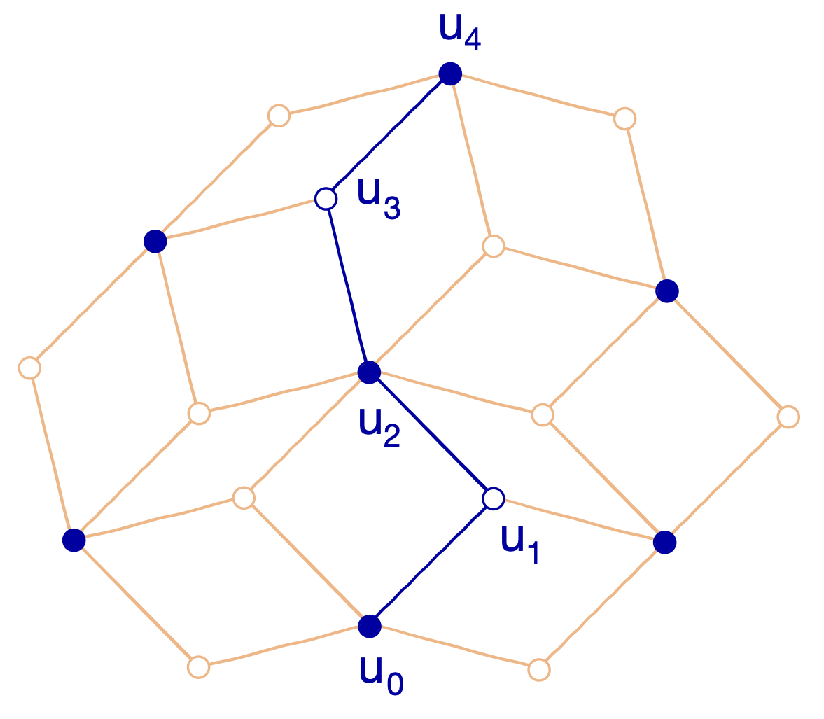
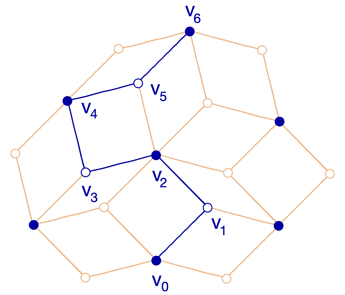
For an integer together with an oriented edge joining a vertex to a vertex set where is the phase of the difference of the coordinates of the vertices; extend this by linearity to 1-chains in , and thus define . Notice that for any oriented rhomb whenever is an odd integer. It follows that for any path , and for any odd integer , depends only on the two end-points of .
Definition 16.
For any pair of vertices and of and for any odd integer , we define where is any path from to .
Note that . In addition .
2.2.2. Train-tracks
Definition 17 (train-track).
A train-track in the rhombic graph is an infinite sequence of rhombs whose consecutive rhombs and are incident along a common edge for each and for which the edges and are parallel for each . We shall denote these parallel edges “train-track tie”, or in short “tie”. We consider train-tracks up to shift and inversion, i.e. is equivalent to if for some . Let denote this set of edges. A train-track has inclination if the ties are parallel to the phase .

Clearly any train-track is determined (but not uniquely) by an initial rhomb together with a choice of one of its edges . For any choice of initial edge in the distance of each edge from the axis determined by is monotonically increasing with ; i.e. the train-track must move forward in the axis perpendicular to .
We say two train-tracks and intersect if for some . Two important features of any rhombic-graph are
Fact 1.
No train-track can intersect itself, i.e. if then for all integers .
Fact 2.
Any two distinct train-tracks are either disjoint or else intersect once.
The notion of train-track is amenable to any quad-graph (a planar graph consisting entirely of quadrilateral faces) and these two properties characterize rhombic graphs within the broader class of quad-graphs; specifically any quad-graph satisfying these two properties is a deformation of a rhombic graph (see [KS14]).
2.2.3. Intersections of train-tracks with paths
A train-track partitions the vertex set into two disjoint subsets and . Specifically, the edge set defines a disconnected subgraph of with two disjoint components; and are the respective vertex sets of these components. Accordingly, we say that two vertices and are separated by if they lie in different components; furthermore we say separates the path if the end-points of the path and are separated by .
Given a path and a train-track let be the set of indices of edges common to both and . If separates then its cardinality must be odd due to the fact the path must begin on one side of and end on the other. If, on the other hand, does not separate then is even (and may in fact be zero if there is no intersection at all).
The edges for are clearly parallel (since they all inhabit the train-track ) but the oriented edges for must alternate in direction and so their phases for must alternate in sign. Consequently, if and is odd then
| (2.4) |
If separates their intersection angle is defined as and is the set of intersections angles of all train-tracks that separate the path . Define the multiplicity for . It follows from equation 2.4 that for odd
| (2.5) |
where and are the beginning and end points of the path . Given a train-track separating with angle of intersection define to be the ray (half-line) starting from in the direction , and be the ray starting from in the direction . It is geometrically clear that must intersect the right hand sides of rays and , without back tracking in the direction orthogonal to (and without intersecting the opposite rays and ). See fig. 9.
For completeness, one should consider the case where lozenges in become infinitely flat, so that goes to infinity in the direction before intersecting (see Fig. 10). Then one can consider that crosses at infinity.
Proposition 3.
Let be a path in , let the direction of the path be . Let us fix the determinations of the angles as real numbers in
| (2.6) |
and let
| (2.7) |
Then
| (2.8) |
In other words, the set and the angle are contained in the open subinterval where .
Proof.
Set . Each is the intersection angle of at least one train-track whose inclination equals (modulo ) and which separates the vertices and .
First let us note that the angle cannot be an element of . Were this the case, there would be train-track joining the righthand sides of the rays and without backtracking. This is impossible, as depicted in figure 11.
Consequently the angles in are in the interval . Consider and . It is enough to prove that . Indeed, suppose instead that . Both and are intersection angles for two respective train-tracks and which separate and . If we attempt to draw and bearing in mind monotonicity and their requisite intersections with the rays , , , and we will observe that the two train-tracks will be forced to intersect at least three times (as depicted on figure 12).
Since two distinct train-tracks may intersect at most once we are forced to conclude that . Finally, by equation 2.5, the difference can be written as
Any positive combination of phases for must lie in the positive cone because . It follows that . ∎
For obvious topological reasons the set only depends on the end-points and of the path . By Proposition 3 if then , which means that if two distinct train-tracks and share the same inclination and both separate then . Consequently the set together with the multiplicities for must only depend on the end-points and of the path as well. This observation is consistent with the fact that the value of depends only on the end-points of .
3. Laplacians and their determinants
3.1. Laplacians and the critical Laplacian
3.1.1. Laplacians associated to polyhedral graphs and triangulations
Given a polyhedral graph G, we denote by , , and
the vector spaces of complex-valued functions supported respectively on the vertices, edges, and faces of G.
The operators , and are associated to a general polyhedral graph G
and were introduced in section 1.2.3.
Each operator is a linear map .
The Laplace-Beltrami operator is defined as
| (3.1) |
The conformal Laplacian is
| (3.2) |
The Kähler operator is
| (3.3) |
, and are respectively the north, south and conformal angles associated to the oriented edge , while and are the circumradii of the respective north and south faces associated to (see figure 1).
Remark 12.
The Beltrami-Laplace operator , the conformal Laplacian , and the David-Eynard Kähler operator on a polygonal graph G agree respectively with , , and when defined on the associated redacted graph (see Def. 8). By definition the vertex sets of G and coincide. So for any pair of vertices the corresponding matrix entries and and are independent of whether we calculate their values with respect to the graph embedding (and incidence relations) of either G or . Likewise , , and operating on G agree with their respective counterparts when defined on any completion of G (see Def. 11).
3.1.2. Areas, angles and circumradii formulas
We recall some basic geometrical formula for these quantities.
Let be a c.c.w. oriented triangle with vertices labelled , , and respective
coordinates , , then the area of the triangle is
| (3.4) |
The circumcenter of the triangle is given by
| (3.5) |
and the circumradius of the triangle is given by the trigonometric relation
| (3.6) |
while the north angle associated to the oriented edge is
| (3.7) |
Furthermore can be written explicitly in coordinates as
| (3.8) |
The derivatives of , and of the angles under a variation of a vertex coordinate are easy to calculate, using for instance
| (3.9) |
and will be discussed later.
3.1.3. Laplacians on critical (isoradial) graphs
The critical Laplacian studied by Kenyon in [Ken02] corresponds to the special case of , with edge weight given by 3.1, defined on a critical graph (according to the terminology of [Ken02]), i.e. an isoradial, Delaunay graph . Accordingly we shall use the following terminology for critical Laplacians, given here.
Definition 18.
Let be an isoradial Delaunay graph. The Beltrami-Laplace operator , the conformal Laplacian , and the David-Eynard Kähler operator (normalized by the squared isoradius of the faces of ) coincide for . This common operator is called the critical Laplacian associated to and is denoted .
| (3.10) |
An explicit formula for is also given in equation 1.14 of Sect. 1.2.3.
3.2. Factorization of Laplacian using and operators
In the case of a planar triangulation T, we present an alternative representation of the operators
and which will be convenient for our calculations.
We follow the definition and the notations of [DE14].
Definition 19.
The operators and are linear operators from the space of complex-valued functions over the set of vertices of T, onto the space of complex-valued functions over the set of triangles (faces) of T.
is defined as follows. Given a triangle (a face of the triangulation T) with vertices , , (listed in ccw order) and complex coordinates for together with a function define
| (3.11) |
corresponds to a discrete linear derivative w.r.t. the embedding because
| (3.12) |
Similarly, its conjugate is defined as
| (3.13) |
and satisfies
| (3.14) |
The transpose of these operators are defined accordingly:
Remark 13.
Note that the discrete derivatives and are defined for general triangulations. Even when the triangulation is isoradial, and do not coincide with the discrete holomorphic and discrete antiholomorphic derivatives and considered in [Ken02] for isoradial bipartite graphs. Indeed and do not even act on the same space of functions than and .
Nevertheless, we shall need to bound the difference between the and the ordinary continuous derivative in the case of a smooth complex-valued function with compact support and its restriction to given by where is the embedding of T. This estimate is explained in Lemma 1 of the introduction and proven in Appendix B.
In addition, the -operator satisfies a discrete analogue of Green’s Theorem
in complex coordinates, namely:
Lemma 3.
Let T be a polyhedral triangulation with embedding , let be a finite collection of triangular faces (each taken with a counter-clockwise orientation), let be the finite subset of (oriented) edges corresponding to the boundary of , and let be a complex-valued function, then
| (3.16) |
Proof.
Use definition 3.11 for and observe that the area defined by 3.4 cancels with the area factor in the denominator of and that for each oriented triangle the term can be reorganized as . Now sum over the faces of . Note that all internal edges count twice with opposite orientations and cancel, and so only the oriented edges on the boundary contributes and give the r.h.s. of 3.16. ∎
The polyhedral condition can in fact be dropped but we assume it to keep the exposition simple. Lemma 3 implies the following corollary which is relevant to our results.
Corollary 2.
Let and be two polyhedral triangulation which share a common redacted graph . Given a face with vertex set let be the set of triangular faces of each of whose vertices are in . Then
| (3.17) |
for any complex-valued function .
Definition 20.
Then we shall heavily use the following local decompositions for the and operators.
Remark 14.
The Kähler operator can be factored as
| (3.19) |
This decomposition is shown in the proposition 2.2. of section 2.6 of [DE14]. Note that and commutes.
Remark 15.
The Laplace-Beltrami operator can be factored as
| (3.20) |
This decomposition can be derived easily using the method of [DE14]. Alternatively one can use the formula 3.4 for and 3.15 to reorganize terms and show that for any one has
| (3.21) |
which amounts to 3.20.
Remark 16.
No similar decomposition holds for the conformal Laplacian , since the weight associated to an oriented edge depends non-additively on the north and south angles and .
3.3. Making sense of the log-determinant for infinite lattices
3.3.1. The problems
As explained in the introduction, we are interested in studying the variation of the under a variation of the coordinates of the triangulation T, where is any of the Laplace-like operators , and . Two potential dangers arise: (1) These operators have zero modes and some care is needed in imposing boundary conditions in order to exclude them. (2) We consider infinite polygonal graphs — and so by any naive account, the log-determinant will be infinite. There is a host of standard methods used to handle these issues; below we discuss two situations where problem (1) and (2) can be side stepped.
3.3.2. Using periodic triangulations:
Consider a polyhedral graph G which is periodic with respect to a lattice with . This means there is an action of the additive group on denoted such that
(1)
(2) and are joined by an edge whenever and
are joined by an edge (moreover the weights of these edges agree)
for all and . Given a choice of an additive subgroup of with , form the quotient graph , which we can view as a finite graph embedded in the torus . Since the edge weights are periodic, the operator descends to an operator on the quotient graph ; moreover if we identify the vertices of with the subset consisting of vertices for which then is a finite dimensional operator acting on vector space of dimension .
We define the reduced log-determinant as the sum of the logarithms of the non-zero eigenvalues of (the non-zero part of the spectrum is real and positive since will be a positive operator in the cases we consider). Then the normalized reduced log-determinant is defined as
| (3.22) |
The normalized log-determinant of , defined for the entire infinite bi-periodic graph G is defined simply as the limit
| (3.23) |
So corresponds to an “effective action” density (free energy density) per vertex on the infinite lattice.
Definition (3.23) agrees with the log-determinant considered by Kenyon in [Ken02] when is the critical Laplacian on a bi-periodic infinite isoradial (critical) graph.
In fact, the limit in formula 3.23 exists and coincides with the following description in terms of matrix-valued symbols: Choose complex parameters and and for each pair define the space of quasi-periodic functions
| (3.24) |
This is a finite dimensional vector space of dimension . Clearly whenever , and consequently the operator restricts to a finite dimensional linear operator on which is called the symbol of . As a matrix the entries of are Laurent polynomials in and , and for generic values of and it will be invertible; indeed the work of Kassel and Kenyon [KK12] implies that its determinant is non-negative for values of and each having unit modulus. One checks that the average value of the log-determinant of this symbol agrees with normalized log-determinant of :
| (3.25) |
Remark 17.
The value of the right hand side of 3.25 can be evaluated using Jensen’s formula (twice) and is independent of the choice of .
3.3.3. Using Dirichlet boundary conditions:
Let us propose the following alternative construction. For a arbitrary polygonal graph G (not necessarily periodic) one can consider a sequence of truncated operators obtained from a nested sequence of domains whose union is : for instance, the sequence of squares ) where is the restriction of the operator to the subset of vertices with Dirichlet boundary conditions imposed on the complement of . This amounts to setting the matrix entry of to zero, whenever . Thus the non-zero part of is a submatrix. Since we choose Dirichlet boundary conditions on the boundary of has no zero modes and is well defined. Then we expect that the normalized -volume log-determinant, defined in analogy with 3.22 by
| (3.26) |
exists, at least in the case of a non-periodic graph G which is sufficiently “regular/homogeneous” (e.g. a quasi-periodic lattice), and agrees with the normalized log-determinant defined above by 3.23 when the graph is periodic. This is to be expected on physical grounds by arguments analogous to those leading to the existence of a unique infinite volume thermodynamical limit for simple classical statistical systems, such as a lattice of classical oscillators, or spin systems, in their high temperature phase, independent of the boundary conditions chosen for the system. We shall not elaborate more, nor attempt to present a complete and fully rigorous proof, since this is not needed for the rest of this work.
3.3.4. Local variation of -volume determinants
The finite variation of -volume determinants (by themselves infinite) under local deformation can be defined properly for the two schemes that we have presented above. Let us explain the idea in the Dirichlet boundary scheme. We begin with a polyhedral graph G and make perturbation by moving some of its vertices inside a finite size compact domain . The operator changes accordingly
If the incidence relations of G do not change, the variation will be an operator supported on the finite set consisting of all vertices in plus their nearest neighbouring vertices (any vertex which shares a common face with a vertex in ). Considering a nested sequence of domains such that , it is clear that one can write the variation series expansion for the restriction of in each
| (3.27) |
In the limit, since the extended to G are equal to , every term in the expansion will converge to its -volume limit, so that we have for any positive integer
| (3.28) |
so that, although and are formally infinite, the difference is finite and one can write
| (3.29) |
We shall study the perturbation around an isoradial, Delaunay graph , where we have seen that (the Green’s function) can be expressed in a simple contour integral form. Moreover we shall consider infinitesimal transformations 1.16, namely
and study the general form of the first order term in 3.29, and some especially interesting terms in the second order term.
3.4. Kenyon’s local formula for
3.4.1. Kenyon’s formula for a periodic infinite lattice
In [Ken02] Kenyon derived an explicit formula for the normalized log-determinant of for periodic, isoradial, Delaunay triangulations . The proof of this result relies only on the structure of the corresponding rhombic graph and indeed works for any rhombic graph. For this reason Kenyon’s formula implicitly extends to all periodic, isoradial, Delaunay graphs . The formula reads
| (3.30) |
where is the volume (number of vertices) of the elementary domain of the infinite periodic graph (see section 3.3.2), the sum runs over all edges in the quotient toric graph, and L is the Lobachevsky function (related to the Clausen function ) defined by
| (3.31) |
3.4.2. Extension to general isoradial (weak) Delaunay graphs
Kenyon’s formula can be formally extended to express the (formally infinite) un-normalized log-determinant for a general isoradial Delaunay graph as a sum over all edges , namely:
| (3.32) |
with for compactness the function of the conformal angles given by
| (3.33) |
We may further generalize this formula to any isoradial weak Delaunay graph obtained from by adding chords inside the faces of , i.e. any graph such that . Indeed, if is a chord in then and where the function is analytically extended to an odd function of over . For any isoradial weak Delaunay graph of this kind, formula 3.32 becomes
| (3.34) |
since the contribution of any chord is zero. This is true in particular for the isoradial, weak Delaunay graphs and mentioned in definition 2 of the introduction. Note that the derivative of is
| (3.35) |
4. The critical Green’s function and its asymptotics
4.1. Kenyon’s formula for the critical Green’s function
The Green’s function studied by Kenyon in [Ken02] is a right-inverse of the critical laplacian characterized uniquely by the following three conditions
1)
2) for
3)
Here is an isoradial Delaunay graph with embedding and its associated rhombic graph (its embedding is also denoted ). Kenyon showed that this critical Green function on is expressed by the explicit integral
| (4.1) |
where is any choice of path from to on and where is the associated sequence of angles. is the meromorphic function in
| (4.2) |
The value of depends only on the end points and of the path; this follows from an argument similar to the proof in demonstrating that the value of for odd positive integers also depends only on the end points and of the path. If we fix and allow the end point of the path to vary then the mapping is an example of a discrete analytic function on as discussed in [Ken02]. By Lemma 5 the restriction of this mapping to vertices may be viewed as a lattice approximation of the continuous exponential function
provided . For this reason is referred to as a discrete exponential function. Finally is any closed, counter-clockwise oriented contour enclosing the finite set of phases . As explained in Proposition 3 the set of angles , and thus , are finite and depend only on the end-points and of the path . The set of poles of the integrand in formula 4.1 is precisely and , so a contour can be chosen which avoids the branch cut of the logarithm; see subsection 4.3 below for details.
Remark 18.
Formula (4.2) is invariant under both global translation and rotation of the graph .
Remark 19.
Let us consider an oriented edge of an isoradial, weak Delaunay graph . There are two possible situations.
- 1:
-
Either is not a chord (see Fig. 13 left) in which case the north and south angles of are equal (and generically non-zero) and both coincide with the conformal angle of the edge .
- 2:
-
Or is a chord (see Fig. 13 right) in which case the north and south angles of are opposite, while the conformal angle of is zero.
In both cases, Kenyon’s formula for the Green’s function for this pair of vertices reads
| (4.3) |
Proof.
Select, for instance, the north face and let be its center. Assume that the isoradius of the critical triangulation is for simplicity. Consider the path . Set and and note that . Then
| (4.4) |
The calculation with the south face gives the same result, regardless of whether or . ∎
4.2. Expansion and bounds for the discrete exponential
Lemma 4.
Consider a finite sequence of angles contained in the closed interval of the form centered about some fixed angle . Using Def. 16), consider
| (4.5) |
Then we have the uniform bound
| (4.6) |
Proof.
Clearly, it is enough to verify the lemma in the case of , otherwise we have where and where .
Begin with the following polynomial and notice that
therefore .
For with the function is clearly continuous and its modulus takes maximal value and so . By construction and so . We now proceed with a yoga of inequalities:
∎
Lemma 5.
Given a finite sequence of angles and the following infinite product expansion of is valid:
| (4.7) |
Proof.
Note that this can be rewritten as
with the the coefficients of a series. ∎
Remark 20.
Let be a finite sequence of angles contained in an interval of the form where is a positive odd integer. Define
| (4.8) |
By Lemma 4 each and is analytic in the unit disk and . Furthermore we have, through the standard combinatorial vinyasas,
| (4.9) |
with the coefficients given by
| (4.10) |
and where the sum is taken over infinite tuples with and such that .
Let and be distinct vertices of and let be a path from to . Translation and rotation invariance of the Green’s function allows us to assume without loss of generality that is situated at the origin and that the phases of the path lie in the open interval ; if not the embedding of may be shifted and rotated to achieve these features; see Proposition 3 for a definition of .
4.3. Contour integral for the expansion
In [Ken02] Kenyon handles the asymptotic behaviour of the Green’s function with respect to the distance using a keyhole contour with a corridor of width avoiding the cut of the logarithm . Paraphrasing Kenyon, this contour runs counter-clockwise along the circle of radius about the origin (connecting ), then travels horizontally above the -axis from to , runs clockwise along the circle of radius about the origin (connecting ), and finally returns horizontally from to below the -axis. Here and (see figure 14). The following lemma allows us to compute the Green’s function by integrating along the cut of the logarithm provided we subtract off the logarithmic divergences.
Lemma 6.
Let be a function which is holomorphic on the extended complex plane outside a subset contained in the interior of the keyhole contour for some values of , , and , and such that then
| (4.11) |
Proof.
where and are the power series expansions of at and respectively. ∎
Corollary 3.
For vertices and in the value of the Green’s function is
| (4.12) |
Proof.
We begin with the observation that for any finite sequence of angles . Since and are vertices in , the length of any path from to in must be even. Thus . Then
∎
4.4. The general asymptotics
Proposition 4.
Proof.
∎
5. Deforming Delaunay lattices and operators
5.1. Setup and problems for deformations of isoradial Delaunay graphs
We start to address the main problem of this work, which is to study geometric deformations of isoradial Delaunay graphs and their associated operators defined in Sect. 1.2.3.
Begin with an initial (not necessarily isoradial) Delaunay graph as defined in Def. 9 with vertex set , edge set , and face set . We deform the initial vertex embedding for by
| (5.1) |
where a positive real parameter and the displacements are implemented by a complex-valued function
with finite support, i.e. a finite subset such that .
If the deformation parameter is unconstrained displaced vertices may potentially collide, i.e. the mapping may fail to be one-to-one. The following simple lemma allows us to avoid this situation.
Lemma 7.
For any pair of distinct vertices the corresponding perturbed coordinates and will always remain distinct provided
| (5.2) |
where
| (5.3) |
Proof.
The mapping has finite support, so the set of pairs such that is finite, and is well defined and finite. The coordinates and are distinct so
provided is non-zero, which is clearly the case whenever . ∎
Definition 21.
Let be a Delaunay graph with embedding and let be a displacement function as above. Let be a value for which the mapping given by 5.1 is one-to-one. The corresponding Delaunay deformation of is the unique Delaunay graph with vertex set for which the map is a planar graph embedding.
Generically, the edge set of differs from the edge set of the initial graph . This is caused by the Delaunay constraints, and this difference can occur spontaneously for . We offer two (not unrelated) examples. Consider first a cyclic face of with vertices. As soon as these vertices may cease to be concyclic. In this case the Delaunay condition imposed on will force the appearance of new edges which will subdivide the initial face into new cyclic sub-faces. An example is depicted on Fig. 15. In the limit these new edges would become chords of the original face if they were adjoined to edge set of (see Def. 6 for the concept of chords and edges of a weak Delaunay graph).
This phenomenon can also occur around intermediate thresholds of the deformation parameter. Two (or more) faces of which are distinct for may become concyclic and merge into a single face (the boundary edges having vanished) when . For this larger face may cease to be cyclic and instantaneously split into sub-faces caused by the appearance of new edges, possibly different from those which existed for . The prototypical example is depicted on Fig. 16. Two triangular faces for merge into a cyclic quadrilateral at and split again along the opposite diagonal of the quadrilateral for . This is, of course, an example of a Lawson flip (well known from flip algorithm used to construct Delaunay triangulations) or, more generally, of a Pachner move on a two-dimensional simplicial complex.
In the next section, we shall discuss how to control this phenomenon of face splittings and edge flips. Let us first introduce two other concepts of graph deformations, which shall be used later.
Definition 22.
Let be an initial, planar triangulation with embedding and let be a displacement function as above. For the triangulation with vertex set and edge set is called a rigid deformation of if the mapping given by 5.1 defines a planar embedding of . In particular this implies that the face set induced by the embedding coincides with the initial face set . Stated simply, no flips are allowed during a rigid deformation.
For a Delaunay deformation the mapping will be an embedding provided it is one-to-one since, by construction, the edges determined by the Delaunay constraints will never cross in the plane. Injectivity can be achieved, for example, by bounding the deformation parameter as prescribed in Lemma 7. For rigid deformations the mapping must be a planar embedding with respect to a predetermined edge set . One way to ensure this is to regulate the deformation parameter so that the area of a triangle given by formula (3.4) remains positive whenever is a triangle of . This is addressed in the following lemma:
Lemma 8.
Proof.
Let us consider a face of with embedding and the deformed face with embedding . Using formula 3.4 for the area of a triangle, and the result 3.15 of Rem. 13, it is easy to show that the area of is related to the area of by
| (5.6) |
is positive and for we have the inequality
| (5.7) |
Therefore implies that , so that the face is c.w. oriented as . This bound is valid for all the faces of . This ends the proof. ∎
Note that the concept of rigid deformation can be extended from triangulations to more general embedded planar graphs, but we shall not need it. We shall, however, use the following concept.
Definition 23.
Let be a Delaunay graph and let a displacement function as above. A Delaunay deformation of as defined in Def. 21 is said to be stable iff is a Delaunay deformation of for all and
| (5.8) |
This means that edges of the initial graph remain edges in and that the deformation creates a common set of new edges in which persist (i.e. do not flip) within the range .
5.2. Keeping control of stable deformations
We now give results which allows controlling stable deformations of Delaunay graphs.
Lemma 9.
Let be an initial planar triangulation with embedding and let be a displacement function with finite support , as in the previous section. Let be a given oriented edge of , and let be its conformal angle defined by 2.1. We do not assume to be Delaunay, so the conformal angle can be positive, zero, or negative. Let and be the adjacent north and south triangular faces of , and let
| (5.9) |
with as in Lemma 7. Take such that
with defined as in Lemma 8 and let us consider the rigid deformation of (which is an embedded planar triangulation by Lemma 8). Let be the deformed conformal angle of the edge in . Then we have the bound
| (5.10) |
with the constant
| (5.11) |
Proof.
Consider the triangulation and an oriented edge with adjacent north and south faces and . Let be the rigid deformation and let
be the corresponding embedding. By 2.1 the conformal angle of the edge in the initial triangulation can be expressed as
| (5.12) |
and the deformed conformal angle in is given by
| (5.13) |
where
| (5.14) |
with
| (5.15) |
and
| (5.16) |
Consider defined by 5.9. Provided that we have
| (5.17) |
Define the function by
| (5.18) |
It is a monotone, convex function on the interval with satisfying
| (5.19) |
Now we use the fact that for any complex number
| (5.20) |
Combining these inequalities, we deduce that
| (5.21) |
We now use this lemma to get our first result for a Delaunay deformation of a Delaunay graph.
Lemma 10.
Let be a Delaunay graph and let be a displacement function with finite support , as above. To each edge of we associate its conformal angle defined by 2.1. Define as
| (5.22) |
and as defined by 5.3 in Lemma 7. Let be the Delaunay deformation of as defined in Def. 21. Then the following bound ensures that the edges of remain edges of , namely:
| (5.23) |
Proof.
The proof uses Lemma 9 and the Lawson flip algorithm.
Given our initial Delaunay graph , let us consider a triangular completion of , as introduced in Def. 11. In otherwords
| (5.24) |
Any completion is a weak Delaunay graph (see Def. 9) and the edges of which are not edges of are chords; consequently
| (5.25) |
for any edge
In general may have multiple (possibly infinitely many) triangular completions. Let T denote the set of triangular completions of , and let us extend the bounds and of Lemma 8 (valid for triangulations) to Delaunay graphs:
| (5.26) |
and then as in Lemma 8
| (5.27) |
Now we start the proof. We choose an arbitrary triangular completion of , and consider the rigid deformation of for bounded by
| (5.28) |
For any edge of notice that
| (5.29) |
and by Lemma 9 we have
| (5.30) |
If the edge of is also an edge of then . Cleary and therefore
| (5.31) |
So the initial edges of still satisfy the Delaunay condition in .
Now we consider whether or not the deformed triangulation is weakly Delaunay, i.e. if
If is weakly Delaunay, it is sufficient to remove all its chords, namely all edges such that . We obtain the redacted graph (see Def. 8) which is a Delaunay graph with the same vertex set as and with embedding . Hence it is the Delaunay deformation of , and it contains the original edges of in light of 5.31. In short
| (5.32) |
If is not weakly Delaunay, there must exist edges of such that
In this case we recursively apply the Lawson flip algorithm to construct from a weak Delaunay triangulation which still completes (see [Law77] and standard textbooks such as [dBCvKO08] or [GH13]). Let us describe the first iterative step.
- (1)
Choose an edge of such that , and consider the quadrilateral made of its north and south faces.
- (2)
Flip the edge , i.e. perform the replacement
so that one obtains a new triangulation .
Some conformal angles in have changed. Specifically
and the conformal angles of the edges , , , and as measured in may differ from their corresponding measures in . The new triangulation is the rigid deformation of another triangular completion of , namely the triangulation with edge set
Therefore and inequality 5.31 is still valid for the edges of , i.e.
The Lawson flip algorithm entails iterating this process: Choose an edge in such that and perform the edge flip to obtain a new triangulation with . Repeat. This process is known to stop after a finite number of iterations, and the final triangulation will have no edge with , and so it will be weakly Delaunay. Clearly is the rigid deformation of a triangular completion of . Now take the redaction by removing any chords. Schematically
The redacted graph is a Delaunay deformation of which coincides with and, to be sure,
as long as the initial bounds 5.28 on are satisfied. ∎
Lemma 10 says nothing about the additional edges which can appear and flip within the initial faces of during the deformation. The following proposition establishes that these additional edges are themselves stable, i.e. undergo no flips, for values of the deformation parameter which are sufficiently small.
Proposition 5.
Let be a Delaunay graph and a displacement function as above. There exists a deformation threshold such that for any the deformation is stable (see Def. 23). As a consequence, the limit of the Delaunay graph when is unambiguously defined, and is denoted
| (5.33) |
is a weak-Delaunay graph sharing the same vertex set and embedding as . Its redacted graph (see Def. 8) is the initial Delaunay graph, i.e. .
Proof.
Let us consider be a triangular completion of (an element of T) and an edge of which is not an edge of (i.e. a chord such that its conformal angle is . Now as in the proof of Lemma 10 consider the rigid deformation of . The deformed conformal angle of is given by
| (5.34) |
with and the north and south vertices for the north and south faces and of the edge in (remember that for this is zero).
is a regular function of (for small enough). We are interested in the values of for which vanishes. Clearly this occurs if ( is taken real)
| (5.35) |
This amounts to solving a quartic real polynomial equation in of the form
| (5.36) |
with
| (5.37) |
P4 has at least one zero (with multiplicity) at , and at most three other zeros, unless it is identically zero. Let us define by
| (5.38) |
For the completion define
| (5.39) |
is strictly positive (possibly infinite) since has finite support on and there are only finitely many chords affected by the deformation. For the initial Delaunay graph define
| (5.40) |
Again has finite support on and since the ’s can only take a finite number of distinct (strictly positive) values it must be the case that is strictly positive.
| (5.41) |
Now define
| (5.42) |
Take within the range
| (5.43) |
and construct according to the proof of Lemma 10. It is weakly Delaunay, hence for each edge. By the argument above, the conformal angles cannot change sign in the interval . Therefore, for any , each conformal angle must stay nonnegative, and so remains weakly Delaunay. This implies that its redacted graph is the Delaunay deformation of and that . In other words, is a stable deformation of .
The graph stipulated in 5.33, exists: it shares the same vertex set and embedding as , while its edge set coincides with for any by stability. In particular each edge of is an edge of while the remaining edges of are all chords. ∎
Remark 22.
The bound (which defines an interval where no flips occur) may be much smaller than . In fact, even for a fixed initial Delaunay graph and a generic displacement function , the threshold may be arbitrarily small w.r.t. . This point will become relevant when discussing the scaling limit and the problem of obtaining uniform bounds with respect to the choice of . We return to this issue in Sect. 8.
Remark 23.
As discussed in the proof of Prop. 5, the edge sets and coincide for . Consequently any stable Delaunay deformation of is also a rigid deformation of the corresponding limit graph within the range . Accordingly the notions of stable and rigid deformation agree for the limit graph provided we work with sufficiently small values of the deformation parameter.
Remark 24.
Since for and since the faces of are cyclic polygons, the conformal angle of any edge is unambiguously defined and strictly positive as varies in the interval .
5.3. Variation of operators under rigid deformations
We now study the variations of the operators , and and of the associated local geometrical quantities arising from rigid deformations (see Def. 22) of triangulations. It will not be necessary to assume that the triangulations are Delaunay at this stage.
Let T be an initial triangulation (possibly Delaunay) with vertex set , edge set and face set (triangles) . Let be the rigid deformation of T induced by the deformed embedding
| (5.44) |
where is a displacement function and where is bounded by the threshold defined in Lemma 8. Recall that and T share the same set of vertices, edges and faces. The deformed discrete differential operators are denoted while the deformed area and radius operators are denoted . They are obtained by making the substitution in formulae 3.11, 3.13, 3.4, and 3.6 respectively. This allows us to unambiguously define deformed versions and of the Beltrami-Laplace and discrete Kähler operators using the factorizations 3.20 and 3.19, namely:
| (5.45) |
We may expand all the relevant operators as (formal) series in (they are in fact meromorphic in ). Up to first order in , the terms in these developments can be compactly expressed using the discrete derivatives and with respect to the triangulation T.
Proposition 6.
The variation of the Laplace-Beltrami operator is
| (5.46) |
Proposition 7.
The variation of the Kähler operator is
| (5.47) |
with the diagonal function and its conjugate which are given for a triangle by
| (5.48) |
Before deriving these two equations, let us note that the variation for is rather simple, while the variation for is more complicated, since we have not found a simple interpretation for the quantities and in terms of the geometry of the triangle .
Proof.
From 3.15, for a pair of vertices and of a triangle in
| (5.49) |
Inserting this in 3.4 gives the variation of the area of the triangle
| (5.50) |
which we can succinctly express as
| (5.51) |
where we view , , and as functions in or, alternatively, as diagonal operators mapping .
Using 3.6 we can write the variation of the circumradius of the face . We write only the leading term of order with the same compact notation and with , and defined by 5.48
| (5.52) |
Similarly, we get the variation of the matrix elements of the operator. At first order
| (5.53) |
When read as operators, formula 5.53 for and its complex conjugate become
| (5.54) |
Combining this with 5.45 and the Leibnitz product rule we get 5.46 and 5.47. ∎
Remark 25.
Remark 26.
There is no such a compact expression for the variation of the conformal Laplacian in the general case. In particular, the variation of the weight associated to an edge will depend on the discrete derivatives of both at the north triangle and the south triangle of the oriented edge , which are a priori independent (see figure 1).
We can, of course, make the substitution in formula 3.7 for the north and south angles (which express the angles as a difference of arguments of edge vectors)
| (5.55) |
where and are the respective north and south vertices of the adjacent triangles and to the edge as depicted on Fig. 1. The order zero and order one terms in the formal series expansion read from 5.49
| (5.56) |
with complex coefficients and given by
| (5.57) |
The corresponding first order variation of the edge weight with can be written explicitly in term of the discrete derivatives and , the coefficients and , and their complex conjugates. We shall not write the formula here, since it lacks the simplicity and geometrical interpretation of our results for and .
5.4. Generic notation for derivatives under graph deformations
We shall use the following compact notation for derivatives and variations of general objects associated to a rigid deformation of a polygonal (Delaunay) graph induced by a deformed coordinate embedding as defined in Def. 22. The object can be a local quantity such as the angle , , associated to oriented edge of G or the area and circumradius of a face . Other objects include the operators , and .
If the object is defined on the unperturbed graph G, the corresponding object on the deformed graph is denoted
| (5.58) |
This is consistent with the notations of Sect. 5.3. The variation of for finite is denoted
| (5.59) |
The initial derivatives w.r.t. are denoted
| (5.60) |
while their evaluations at zero are denoted
| (5.61) |
Accordingly, the Taylor expansion of reads
| (5.62) |
The terms of order obtained in the previous section 5.3 give the explicit formula of the first derivatives for the objects considered there. We do not rewrite them explicitly.
6. Variations of log-determinants
6.1. First order variations of determinants
6.1.1. The setup
Here we compute the first order term in the -expansion of the (formally infinite) logarithm of the determinant of . This first order term is on general grounds
| (6.1) |
The results are each expressed as a sum of local terms over the weak Delaunay graph arising from the critical graph and the displacement function . For both the Laplace-Beltrami and Kähler operators, there is a local term associated to each edge of ; there is an additional local term attached to each face of for the Kähler operator. In the case of the conformal Laplacian the local terms associated to chords of differ from local terms of the regular edges of . For this reason formula 6.5 is expressed as two sums: one over the regular edges and another over the set of chords .
6.1.2. The results for first order variations
We first give the results; their derivations are given in the following sections.
Proposition 8.
Laplace-Beltrami. For the Laplace-Beltrami operator , the first order variation of with respect to the deformation 5.1 can be expressed simply in terms of the variations of the north and south angles and of edges .
| (6.2) |
The function , given by 3.35, is the derivative of the function given by 3.33. and are given by 5.56.
Remark 27.
Owing to the extended form 3.34 of Kenyon’s result for , it is interesting to note that, up to terms of order , can still be written as a sum of local terms involving the local geometry of the deformed Delaunay graph , similar to Kenyon’s result although the graph is not isoradial
| (6.3) |
Remark 28.
Proposition 9.
Conformal Laplacian. For the conformal Laplacian , the first order variation of with respect to the deformation 5.1 can also be expressed simply in terms of the variations of the north and south angles and of edges . However, we must distinguish between the contributions made by regular edges versus chords in . Keep in mind that the set of regular edges coincides with the edge set of the critical graph.
| (6.5) |
where is the derivative of the function
| (6.6) |
and where is the Lobachevsky function defined in 3.31. Remember that is the conformal edge angle for general triangulations.
Remark 29.
Up to order , can still be written as a sum of terms reflecting the local geometry of the weak Delaunay graph . (see 5.1).
| (6.7) |
Proposition 10.
Kähler operator. For the Kähler operator , a local formula also holds at order . It involves the variations of the angles and for edges , but also the variations of the circumradii for faces . We note that .
| (6.8) |
Remark 30.
Up to order , can still be written as a sum of terms reflecting the local geometry of
| (6.9) |
Again, we obtain a nice local expression involving the angles and and the circumradii . Like the conformal Laplacian, the global conformal invariance properties of the Kähler operator are not evident in the result. However, concyclic configurations and chords do not play any special role.
6.1.3. Proof of Proposition 8
We first consider the variation of the Laplace-Beltrami operator under a deformation of the form 5.1. One can use 5.46 to compute explicitly the first order variation of , but it is simpler to start from its definition in terms of angles 1.11. For an edge of
| (6.10) |
This implies that the variation is
| (6.11) |
where and are of order . The limit graph is weakly Delaunay and isoradial so either or . In both case so that at first order
| (6.12) |
It remains to combine this with the propagator which for regular edges of is
| (6.13) |
A similar relation is in fact valid for chords of
| (6.14) |
Thus the first order variation is
| (6.15) |
This, together with 3.34, leads to 6.3, and this ends the proof of Proposition 8.
6.1.4. Proof of Proposition 9
For an edge of the matrix element the conformal Laplacian is
| (6.16) |
This implies that the variation is
| (6.17) |
Keep in mind that the limit graph is weakly Delaunay and isoradial and so either or . The first case corresponds to a regular edge, while the second case corresponds to a chord. Thus to first order in the matrix entry is
| (6.18) |
The first order variation of the log-determinant reads as a sum over the edges of , but it is different for the edges in and the chords of . Combining with 6.13 we get at first order
| (6.19) |
with the function given by
| (6.20) |
6.1.5. Proof of Proposition 10
The variation of the Kähler operator starts from the expression of the matrix elements of an edge in terms of the angles and and of the circumradii and given by 1.12, namely
| (6.21) |
Its variation is therefore
| (6.22) |
For an isoradial triangulation (critical case), , therefore one has . Thus in the critical case, the contribution made by the first term in 6.22 to the variation is
| (6.23) |
The second term’s contribution can be reorganized as a sum over faces of , i.e. counter-clockwise oriented triangles
| (6.24) |
Using the fact that and that for the critical case
and the fact that for a triangle , one has
we obtain
| (6.25) |
6.2. Second order variations
6.2.1. Principle of the calculation
In order to probe the second trace term in the perturbative expansion 1.19, we consider a bi-local deformation of the underlying critical graph with an embedding of the form
| (6.26) |
where is a pair of independent deformation parameters and where are two functions, with finite supports and in and whose respective lattice closures and are disjoint; see 1.17. To insure that is a stable Delaunay deformation, we restrict the parameters within the range where and are the thresholds dictated by Proposition 5. Furthermore we shall assume that the distance between the two supports is large, i.e. where
| (6.27) |
We want to isolate and then examine the long-range behavior of the cross-term occurring within the perturbative expansion of the log-determinant, namely in
The first trace term contributes nothing of order since the lattice closures of the supports and are disjoint. The only non-vanishing contribution comes from the second trace term
| (6.28) |
which is bilinear in the total variation . Accordingly, the coefficient of can be expressed as
| (6.29) |
where and are first order variations of the Laplace-like operator following the notations set in Sect. 5.4. The sum on the left hand side is taken over vertices , , , such that both matrix entries and are non-zero. In particular this implies that is an edge in with vertices . Likewise must be an edge in with vertices .
Provided the two zones of support and are far enough apart, the matrix entries and of the critical Green’s function will only involve pairs of vertices with and . Under these circumstances we may estimate the contributions made by these matrix entries using the asymptotic expansion 1.15 for the Green’s function.
It will be convenient to take a triangular completion of the deformed Delaunay graph as defined in Def. 11. Likewise will be the completion of the limit graph induced from . This will allow us to use the variational formulae 6 and 7 for the Laplace-Beltrami and Kähler operators. In general such a completion will not be unique. Nevertheless the redactions satisfy and regardless of the choice of completion. The Laplace-Beltrami operator, Kähler operator, and the conformal Laplacian will not be affected by this choice, since the weights assigned by the operators to any chords, introduced by the completion, must vanish.
6.2.2. The Laplace-Beltrami operator
The simplest case is the Laplace-Beltrami operator. We shall need two intermediate results.
Lemma 11.
Let be a c.c.w. oriented triangle with circumcenter and circumradius . Define for . Let be the matrix elements of the discrete derivative operator restricted to the triangle . For any integer one has the uniform bounds
| (6.30) |
and
| (6.31) |
Proof.
Using the definition 3.11 of one can rewrite
| (6.32) |
For we can rewrite the numerator as
| (6.33) |
which involves a special case of the following Vandermonde-like determinant:
| (6.34) |
where is the complete homogeneous symmetric polynomial of degree (a Schur polynomial),
| (6.35) |
which consists of monomials. The numerator equals the denominator in the r.h.s. of 6.32 when and since we get
| (6.36) |
when . It is clear that for we have the bound
| (6.37) |
which is saturated when . For or it is clear that . When , we can rewrite
| (6.38) |
by a similar trick. Since we get the bound
| (6.39) |
Thus we get 6.30. To obtain 6.31 one uses simply
| (6.40) |
and 6.30. ∎
Now we can get uniform asymptotic estimates for the discrete derivatives of the Green function.
Lemma 12.
Let be the critical Green’s function on an isoradial, weak Delaunay triangulation , let and be two faces (triangles), and let and be the complex coordinates of their respective circumcenters and . Let be the distance between the centers. Then the discrete double derivatives of the Green function have the following large distance asymptotics
| (6.41) |
and
| (6.42) |
Proof.
Let and be the vertices of and respectively. The triangulation is isoradial, so denote () and (). Use 1.15 to separate the Green function into its leading large distance term (continuous limit term) of order , its subleading large distance correction of order , and the rest of its large distance expansion of order .
| (6.43) |
with
| (6.44) |
Begin by writing
| (6.45) |
and expand the logs and powers of and in formulae 6.44 as power series in and where is large. For example:
The coefficients in these expansions involve the phases and and so the matrix entries in formulae 6.41 and 6.42 can be computed using the basic identities
| (6.46) |
along with values of , and , explicitly given in 3.11 and 3.13). As an illustration:
The vanishing of the coefficients of order is straightforward. We present the calculation of the coefficient of occurring in here:
Thanks to Lemma 11 (or in this case through a direct estimate) its norm is uniformly bounded by a constant independent of the shape of the faces. For , which is a smooth function of the vertex coordinates, these calculations amount to replacing and by their corresponding continuous derivatives and , up to subdominant terms of order . This is in agreement with Lemma 1. The result is that the asymptotics 6.41 and 6.42 are valid for alone.
To end the proof of the lemma, one must show that the corresponding derivative terms for and are . This is clear for , which is itself , hence its discrete derivatives are also . But this is not obvious for which is only . We must use the explicit form of . Let us consider the term
which appears in . One has
So we have to consider three terms. The first term is
In the last step we used the uniform bound from Lemma 4
The second term is
From Lemma 11
hence the second term is of order . By the same argument, the third term is
This ends the derivation of 6.42 (the second equation is the c.c.). The derivation of 6.41 proceeds in a similar way. ∎
We are now in a position to state the main result.
Proposition 11.
The second order variation for the Laplace-Beltrami operator on an isoradial, Delaunay graph is
| (6.47) |
where the double sum is taken over pairs of triangles such that all vertices of reside in and all vertices of reside in .
Proof.
We start from the local form of the operator 3.20, which implies that the first order variation on is
We use the formula for the variation of
as well as the formulae for the variations of the and operators given by 5.54, which read
to get
| (6.48) |
One uses this and the cyclicity of the trace to rewrite the second order variation as
Note that the trace on the l.h.s. is a sum over vertices, while the trace on the r.h.s. is a sum over faces (triangles). Using the large distances asymptotics 6.41 and 6.42, and writing the trace explicitly as a double sum over faces and gives the theorem. ∎
We now consider the other operators. The case of the conformal Laplacian is more complicated, so let us first discuss the Kähler operator.
6.2.3. The Kähler operator
Proposition 12.
The second order variation for the Kähler operator on an isoradial, Delaunay graph has the same form as the second order variation for the Laplacian
| (6.49) |
where the double sum is taken over pairs of triangles such all vertices of reside in and all vertices of reside in
Proof.
The derivation goes along the same line. We start from Prop. 7 which gives the explicit form 5.47 of the first order variation of . The graph is isoradial, so all circumradii are equal and thus
This implies that the first order variation of has the special form
| (6.50) |
with and defined by 5.48. Formula 6.49 follows by repeating the analysis made in the proof of Proposition 11, which relies on the asymptotics of Lemma 12. One can check that the new terms involving and do not change the asymptotics 6.47 obtained for . ∎
6.3. The case of the conformal Laplacian: the anomalous term
6.3.1. Second order variation for the conformal Laplacian
By formula 6.18 in the proof of Proposition 9 the contribution made by regular edges to the first order variation of the conformal Laplacian is identical to the variation of the Laplace-Beltrami Laplacian. There is, however, an additional term in the first order variation coming from the chords of . We call it the “anomalous term” and denote it :
| (6.51) |
The non-diagonal elements of are non-zero only for chords. From 6.18, for vertices , they are
| (6.52) |
Here is an edge of and is an orientation. The graph is isoradial and weakly Delaunay and so for any edge. In particular and so where is the opposite orientation. As for the diagonal terms we have
| (6.53) |
In the case of a chord we may use 5.56 for the angle variations and and re-express the anomalous term given in formula 6.52 as
| (6.54) |
where the functions and are defined in 5.57 and where and are the respective north and south triangles abutting in the triangulation which completes .
The second order variation
| (6.55) |
is the sum of the second order variation made by the Laplace-Beltrami Laplacian, namely
| (6.56) |
along with three anomalous trace terms which we can express (in light of 6.53) as follows:
| (6.57) |
where and are oriented edges of the triangulation whose vertices and lie in and respectively and where
| (6.58) |
Note that where has the reverse orientation. Applying two rounds of formula 3.15 we obtain
| (6.59) |
where is a triangle of , north or south, containing the edge for . By assumption and are separated by a large distance and so we can estimate as presented in formula 6.59 using asymptotic expansions 6.41 and 6.42 of Lemma 12. We end up with
| (6.60) |
where as introduced in Definition 16.
6.3.2. The chord-chord term
Let us begin by examining the chord-chord term of 6.57. It involves the contribution of two (oriented) chords and whose vertices of and are contained in and respectively. Since is a chord for in the corresponding north and south triangles and in are concyclic and therefore share a common circumcenter whose complex coordinate we denote . This is depicted in Fig 17.
Putting things together, we see that the contribution made by a pair of (oriented) chords to the chord-chord anomalous trace term in 6.57 is
| (6.61) |
with and given by 6.54, that we recall for completeness.
with
and a similar form for . Any triangulation which completes the limit graph is itself isoradial and weakly Delaunay consequently the value of which is given by 3.8.
The result 6.61 for the anomalous chord-chord contribution to the variation of does not have the same form as the “regular” contribution 6.56 which is similar to the variation of the Laplace-Beltrami operator , which is a sum over triangles of terms
First, besides harmonic terms in the coordinate of the circumcenters of the form
it contains non-harmonic terms of the form
which are problematic with conformal invariance and an interpretation in term of CFT, as will be discussed in Sect. 9.
Second, from the form of and , it does not contain only terms of the form
but also terms of the form
Third, the geometric terms associated to the faces (the triangles and ) are not simply the area terms and , but they depend of the detailed geometry and orientation of the chords and the triangles through the terms and .
6.3.3. The chord-edge term
We now discuss briefly the chord-edge term present in 6.57 which involves the anomalous variation term of a chord and the ordinary variation term of an edge . It will be simpler to group together the terms made by a single chord and the edges forming the boundary of a fixed (counter-clockwise oriented) triangle and then sum the contributions as the chord in and triangle in both vary; see the illustration in Fig. 18.

Accordingly, the contribution made by a chord-triangle pair is found to be
| (6.62) |
This term is again different from the regular term. Now it is harmonic in the coordinates of the circumcenters, since it does not contain the non-harmonic term
However, it still contains the terms of the form
and it depends on the detailed geometry and orientation of the chord, as for the chord-chord term discussed previously.
6.3.4. A simplification for specific deformations
Finally, let us note that the anomalous term for a chord 6.54 takes a simpler form in the special case when the discrete derivatives of coincides on the north and south triangles and
thanks to the following lemma,
Lemma 13.
Consider two triangles and sharing the edge and the flipped triangles and sharing the edge as depicted on Fig. 19. Let be a function defined on the vertices. Then the four following equalities are equivalent
| (6.63) |
Note that the four points are not necessarily concyclic.
Proof.
In this case, a single pair of discrete derivatives of is associated to a cocyclic configuration of points, namely a simple cyclic polygon () with circumcenter . The variation for a chord is then given by
| (6.64) |
6.4. Curvature dipoles and the anomalous chord term
Let us discuss a possible explanation of the anomalous terms corresponding to deformations of cocyclic vertex configurations. The adjective "anomalous" indicates that these contributions are not present for either the Laplace-Beltrami operator or the Kähler operator , both of which admits a smooth continuum limit consistent with the predictions of conformal invariance.
As discussed in the definition 1.12 the conformal Laplacian for a Delaunay graph G can be viewed as the discretized Laplace-Beltrami operator on the rhombic surface introduced in Def. 15. The construction of is illustrated in Fig. 20 for an isoradial Delaunay graph G and in Fig. 21 for a generic (non-isoradial) Delaunay triangulation G.


It is easy to see that the surface is piecewise flat, with curvature defects (i.e. conical singularities) localized at the vertices associated to circumcenters of faces in G. The defect angle corresponds to a localized curvature defect at and its value is given in terms of the conformal angles of the edges forming the boundary of the face . Recall from 2.3 that the associated scalar curvature at a vertex is
| (6.65) |
or equivalently twice the measure of the defect angle around the circumcenter of the face , i.e. the Gauss curvature
| (6.66) |
For an isoradial Delaunay graph G the rhombic surface coincides with the planar kite graph whose faces, in this case, are all rhombs. Furthermore, the scalar curvature associated to each face in G is zero. For a generic Delaunay graph G the scalar curvature will be non-zero (see Fig. 21). Indeed, consider a cyclic quadrilateral face in an isoradial triangulation depicted in Fig. 22 and the effects of a generic deformation depicted in Fig. 23. In four lozenges meet at where the scalar curvature vanishes.


As illustrated in Fig. 23, as soon as we deform this cyclic quadrilateral, a diagonal edge generically emerges in (infinitesimally a chord in ) which subdivides the quadrilateral into two triangles and , while the circumcenter splits into two circumcenters and . In the deformed rhombic surface a new lozenge appears between and . However this new lozenge is “flat” i.e. to first order in its angles are . Therefore the Gaussian curvatures and have opposite sign and they are both of order , not of order . In terms of the north and south angles of the chord they read
| (6.67) |
Thus the deformation produces a curvature dipole associated to the chord , i.e. neighboring curvature defects with non-zero but opposite signs. Said differently, the smooth deformation manifests a discontinuity in the curvature. Generically when one smoothly deforms a cyclic face of with four or more vertices, a curvature dipole will emerge for each chord which subdivides the face .


Finally, let us stress that a curvature dipole appears if the anomalous term discussed above in 6.3.1 is non-zero. Indeed this anomalous term is proportional to , while the dipole is proportional to . Thus for a chord with , no anomalous term is present and so no curvature dipole appears at first order in the deformation. This occurs iff the circumcenter of the face lies on the edge . Notice that if is a quadrilateral (as in Fig. 23) where the north and south angles of both and the flipped edge are zero then the face is a rectangle. In this case, to first order in , the deformation is , not . These deformations are the ones considered by Kenyon in the seminal paper [Ken02].
7. The scaling limit of variations
7.1. Rescaling smooth deformations
As explained in the introduction, we incorporate a scaling factor into the deformation in order to define and study a continuum limit. We may view the scaling parameter as imparting a resolution on the critical graph, i.e. we get a rescaled embedding of , under which vertices become closer and denser in any compact region of the plane as increases. In particular the area of a face shrinks by a factor of under the rescaled embedding while its circumcenter coordinate is rescaled by a factor of . In this way, the scaling parameter allows us to interpret the critical graph as a planar partition and can be used to define a Riemann sum. More specifically, given any continuous complex-valued function with compact support then
| (7.1) |
Given a smooth complex-valued function with compact support, and a scaling real parameter, we set . When deforming a critical isoradial Delaunay graph (with unit circumradius ), we shall consider the restriction of to (the coordinates of) the vertices of the critical graph. By abuse of notation, we shall write for each vertex . We use to displace the coordinates of the critical graph and define a deformed embedding, namely
7.2. Rescaling bi-local deformations
Our analysis of second order variations (for the log-determinants which we consider) involve a bi-local deformation implemented by two smooth, complex-valued functions and whose respective supports and are compact and have lattice closures and which are disjoint. Set
to be the distance between the supports and . Obviously . The corresponding deformed embedding of the critical lattice is given by
where is a pair of deformation parameters and where we use the notation and by abuse of notation for a vertex and . The results of Lemma 5 still hold for the bi-local deformed embedding ; simply apply the Lemma to and independently and take . Let us denote by the Delaunay graph uniquely determined by the vertex set together with the deformed embedding . As we have seen, the one-sided limit for induces the structure of a weak Delaunay graph on the vertex set with respect to the critical embedding . In general, the edge set will vary as the scaling parameter evolves; nevertheless for all . For each value of select a weak Delaunay triangulation which completes . Because for each we may always perform the following resummation
| (7.2) |
where we combine terms on the left hand side involving triangles of which share a common circumcenter and where is any quantity which depends only upon the circumcenter of . Consequently the choice of triangulation completing will not affect our calculations.
7.3. Scaling limit and derivation of Theorem 2
We now are in a position to study the scaling limit of the bilocal deformation terms 6.47 (Prop. 11) and 6.49 (Prop. 12)) and to derive Theorem 2. For or let denote the subset of faces of G whose vertices belong to the lattice closure of the support for .
7.3.1. The initial finite term
Let denote either the Laplace-Beltrami operator or the Kähler operator on the Delaunay graph . From prop. 11 and 12 the cross-term of is given by the trace term
| (7.3) |
which can be expressed as the following double sum over triangles in
| (7.4) |
where is the circumcenter of for . Both and have compact support so by Lemma 1 we have that where is bounded by a constant independent of both and . We begin by breaking 7.4 into two pieces and evaluate their large limits separately.
7.3.2. The subleading term
The large limit of the second part of 7.4, vanishes as the following computation shows:
| (7.5) |
In the large limit the sum over the triangles becomes a standard Riemann integral
| (7.6) |
Hence
| (7.7) |
7.3.3. The leading term
To evaluate the first part in 7.4 we consider the norm of the difference between the original term with discrete derivative and the corresponding term with continuous derivatives, and use the previous results to get the bounds
In the large limit each sum over triangles becomes a Riemann integral, hence the large limit of the l.h.s. of 7.3.3 is bounded by
| (7.23) |
7.3.4. Summing up
From this it follows that
| (7.24) |
7.4. Controlling the geometry of the lattice for small deformations
7.4.1. The limits we considered
Let us summarize what we did previously, up to sect. 7.3. We begin with an infinite critical graph and two displacement functions and whose respective supports and are compact and whose lattice closures and are disjoint. We construct the stable Delaunay deformation with embedding along with a corresponding deformed operator where is a pair of independent parameters. We then proceed to isolate the coefficient of in the Taylor series of . Since the lattice closures of the supports of and are disjoint the first trace term contributes nothing. The only non-vanishing contribution to comes from the second trace and can be expressed as
| (7.26) |
defined on the weak Delaunay graph (a completion of the isoradial refinement of the initial graph relative to the deformation). We then rescale the deformation by and consider the family of deformations and show the scaling limit of 7.26 exists and is independent of the choice of initial critical graph . Stated simply, we study the nested limit
| (7.27) |
An interesting question is whether these two limits can be interchanged. A positive answer would be a first step in understanding if one can define a continuum limit of (the total variation of) starting from an infinite Delaunay graph which is not isoradial, but rather obtained by a small, smooth deformation of a Delaunay graph which is isoradial. A simpler question is the following: We know that for a given critical graph , the limit 7.27 makes sense when . Is the convergence uniform w.r.t. all critical graphs ? We return to this issue in Section 8.
7.4.2. The problem with flips
The geometrical effects of a finite -deformation of a Delaunay graph G have already been discussed in Sections 5.1 and 5.2. Lemma 9 and Prop. 5 ensure that, for a given initial graph and a given displacement function (with compact support), there exist a strictly positive bound such that no flip occurs in the interval . However depends non-trivially on and on the geometry of . Furthermore it is clear that such a bound cannot be made uniform w.r.t. all critical graphs . This means that given any small value of the deformation parameter, flips will occur in for some critical graph within the class of all critical graphs. Consequently the (matrix entries of the) operators are discontinuous functions of , and it will be difficult to control them as varies.
7.5. A simple restriction to control small deformations: enforcing a global lower bound on the edge angles
A naïve but brutal way to manage the “flip problem” is to consider only a subclass of graphs such that the bound of Prop. 5 can be controlled explicitly, so that no flip occurs. Similar constraints 7.30 on the geometry of have been used in the literature for other problems involving isoradial lattices, see e.g. the paper by U. Bücking [Büc08]. Our solution is given by the following Lemma.
Lemma 14.
Let be a non-zero, smooth complex-valued function with compact support . We define
| (7.28) |
This is a simple modification of the bound of Lemma 7 given by 5.3 which is now independent of the triangulation. For a generic Delaunay triangulation T we define, in analogy with given by 5.22 in Lemma 10,
| (7.29) |
For a fixed, strictly positive , define the subset of Delaunay triangulations
| (7.30) |
and the strictly positive bound
| (7.31) |
with as in Lemma 9.
For any triangulation and any scaling parameter , the Delaunay deformation of T preserves all the edges of T if .
| (7.32) |
In other words, no flip occurs as long as .
Proof.
The mapping is an embedding provided there are no “collisions”, that is whenever are distinct vertices in . Equivalently must not vanish. Apply the fundamental theorem of calculus using .
By construction and taken together with the fact that we can conclude that . As long as we can apply Lemma 10 and conclude that the edge set . Since T is a triangulation no chords appear and hence . We stress that this bound on is valid and independent on all values of the scaling parameter, including .
∎
8. Finite variations, beyond the linear approximation
8.1. Outline of the section
In this section, we now consider deformations of an initial critical lattice implemented by a local diffeomorphism of the plane
for small values of a deformation parameter , and a fixed smooth (but non-analytic) displacement function with compact support. We shall look for uniform bounds for the variation of the operators and with respect to , independent of the particular geometry of the initial critical graph , except for its isoradius .
We therefore need to consider generic Delaunay deformations and take into account the occurrence of edge flips in the deformed Delaunay graph . These flips were avoided in the stable deformation scheme studied in sections 5, 6 and 7 by imposing tight bounds on the parameter .
For a fixed smooth displacement function and a deformation parameter , it will be necessary to compare the corresponding Delaunay and rigid deformations, as explained in Sect. 5. We discuss this in sect. 8.2, as well as the concept of “backtracking a deformation without flips”.
In Sect. 8.3 we give explicit variational formulas for the various operators , , and as well as the circumradii in the case of a rigid deformation of the graph; see Def. 22.
In Sect. 8.4 we derive integral representations of the variations of these objects taking flips into account.
In Sect. 8.5 and 8.6 we give variational formulas for the discrete derivatives and as well as the circumradius of a face. The later result, given in Prop. 13, is important and leads to uniform bounds on the variations of , , and with respect to ; see Prop. 14.
In Sect. 8.7 we deduce strong results on the uniform convergence of the scaling limit for (prop. 15 and 16) and of the scaling limit of the corresponding second order bi-local trace term (which leads to the OPE) (prop. 17).
In sect. 8.8 we finally address the problem of interchanging the deformation limit and scaling limit when evaluating the bi-local trace term of . Specifically we consider the scaling limit of the bi-local term in the variation of for non-zero deformation parameters. The uniformity of this limit depends on a technical bound on the discrete derivatives of the function defined for isoradial graphs by 2.5. We explicate this condition and conjecture that the bound is valid for general isoradial graphs in Conjecture 3. Provided the bound is satisfied, we prove in Prop. 17 that the bi-local trace term has a uniform scaling limit, and that the scaling limit and the deformation parameter limit both exist, are uniform, and commute (see Prop. 18).
Finally, in Sect. 8.9 we address the same questions for deformations of the Kähler operator . Prop. 19 gives a uniform bound on the variation of , but it implies that there is no general scaling limit for for non-zero values of the deformation parameters (Prop. 20). This is different from the situation for . We argue that the best uniform convergence result to be expected for the bi-local trace term is a scaling limit where both and simultaneously, keeping constant (Prop. 21).
8.2. Deforming triangulations with and without flips
We now define and compare Delaunay deformations of graphs and connectivity-fixed deformations of the same graphs.
8.2.1. Delaunay deformations (with flips)
We start from an (isoradial) Delaunay graph and then deform its embedding using a smooth function with compact support to obtain a mapping
| (8.1) |
for vertices of . Using the method for proving Lemma 7, it is simple to prove that the mapping defines an embedding of the vertex set as long as is small enough, namely:
| (8.2) |
Indeed we have
This ensures that if , at least as long as 8.2 holds.
As in Def. 21, the Delaunay graph is obtained by applying the Delaunay construction to the set of deformed coordinates for . The vertices of and are identical by definition, however the edges and the faces of may differ from those of since the Delaunay constraints may force flips to occur during the deformation. Unlike the setup of Lemma 10, the inclusion may now fail. Generically will be a triangulation regardless of whether the initial graph is a triangulation.
, and are the Laplacian operators relative to the lattice , and act on the same space of functions irrespective of since, by construction, the vertex sets agree. Similarly, we denote by and the discrete derivative operators relative to the faces of , both of which are operators . Note that, in general, the set of deformed and critical faces differ, i.e. . Similarly we denote by and the area and circumradius functions for the faces of .
8.2.2. Geometric Back-Deformation: deforming without flip
We define the rigid back-deformation of the Delaunay graph to be the graph whose vertex set and embedding are identical to those of our initial (weak) Delaunay graph , but whose edge and face sets coincide with those of the Delaunay graph obtained from by a Delaunay deformation. The construction of can be seen in two stages:
- (1)
First is the end point of the continuous family of Delaunay deformations
obtained by continuously deforming the embedding of the initial graph over the range while maintaining the Delaunay condition (and performing edge flips as required) at each stage of the deformation.
- (2)
Then, starting with , reverse the deformation by letting move from to
but without performing any edge flips. In general will denote the graph whose vertex, edge, and face sets coincide with but whose embedding is .
More schematically
| (8.3) |
It is clear that is a graph (and in general a triangulation) with the vertex set as the original Delaunay graph , but is generically not a Delaunay graph.
8.2.3. An illustrative example
Let us give a simple but illustrative example of such deformations of a triangulation .
The original triangulation is a biperiodic lattice. Vertices are labelled by with coordinates
Hence the Delaunay triangulation is made of “thin” up and down triangles such that
We choose as deformation function a simple shear parallel to the real axis, so that the deformed coordinates of vertices are
The effect of a Delaunay deformation is depicted on Fig. 24, on the special case of , and for . Note that a flip occurs for every
and that the Delaunay deformation is then periodic
Note also that if
a large number of flips occur, even when is small.
The corresponding no-flip back-deformation which send back is depicted on Fig. 25. It is clear on this figure that no back-flip occurs at , so that an original face of stays a face of . However is a triangulation which is not Delaunay anymore.
8.3. Full variation of operators without flips
8.3.1. Variation of the area
Consider the variation of the triangulation given by deforming the embedding without flips (so that in fact should be denoted with the notations of the previous section). For a triangle the full variation of its area is from 3.4 and 3.15
| (8.4) |
For brevity will denote the scaling factor
| (8.5) |
8.3.2. Variation of the discrete derivatives
The vertex sets and are, by definition, identical and the face sets and agree so long as no flips occur in the deformation . Consequently the nabla operators and (and their conjugates and ) share a common range and domain. Accordingly we have:
| (8.6) |
8.3.3. A word of caution: deformations of functions
Recall that we may restrict a smooth, complex-valued function to the vertex set of the triangulation T using its graph embedding . Bearing some abuse of notation, we define and denote this restriction by for vertices . Some care is needed when restricting a smooth function to the deformed triangulation . The vertex sets of T and are identical but, of course, their respective embeddings and are not, and consequently the functions and do not agree. In order to side step this discrepancy we introduce a deformed, smooth function defined implicitly by
| (8.7) |
for all , where is fixed and sufficiently small. By construction,
| (8.8) |
To stress the role of the deformed embedding we shall define and denote for . When this allows us to write
| (8.9) |
8.3.4. Variation of the circumradii
The full variation of the circumradius of a face is more complicated. For a face with vertices labelled i.e. using 3.6 we get
| (8.10) |
with
| (8.11) |
where for an (unoriented) edge denotes
| (8.12) |
8.3.5. Variation of the operators
Thus we get the variation of the Laplacian operators from
| (8.13) |
| (8.14) |
that we do not write explicitly. Note that all the expression we got are rational functions in , and that when keeping only the first order in in a series expansion, we recover the results of Sect. 5.3.
8.4. Full variation of operators under Delaunay deformations (with flips)
Here we address the case of a critical triangulation with isoradius whose embedding undergoes a deformation
where flips are allowed, so that the deformed graph remains Delaunay. As before the displacement function is the (restriction) of a smooth complex-valued function on the plane with compact support. We consider the full variation of the operators associated to the deformation , namely
| (8.15) |
instead of the instantaneous, first order terms and in the respective -expansions as done in Sect. 5.3 and 6. We shall need uniform estimates for the limit of terms related to the variations and which are independent of the initial critical lattice . Furthermore uniform estimates for the limit will be needed, as this is synonymous with the scaling limit.
Unfortunately, the exact results of the previous section 8.3 cannot be directly applied, since flips generically occur within the continuous family of Delaunay graphs as the deformation parameter moves from zero to . Nevertheless, we may write each variation as the integral of a derivative, and then try to get uniform bounds on the derivatives. This is what we discuss in the remaining part of this Appendix.
Let us first consider the simpler case of the Laplace-Beltrami operator . We can write
| (8.16) |
Indeed, since is smooth with compact support, there is a finite (possibly large) number of flips as increases, and we know that is a continuous function of , and its derivative exists and is continuous in the interval between the flips. Therefore the derivative is bounded and piecewise continuous, so that the integral 8.16 makes sense. For a given value , the first order term in formula 5.46 extends to the case of defined on and w.r.t. the transported displacement function in the plane.
| (8.17) |
with
| (8.18) |
Similarly, we can write the variation of the Kähler operator as
| (8.19) |
The results of Section 5.3 give for the derivative of
| (8.20) |
with
| (8.21) |
and with the and defined by 5.48 for faces the triangulation , namely for a face ,
| (8.22) |
Note that we can decompose as a sum of the terms defined in 8.12 for edges of . Specifically where .
8.5. Uniform bounds under Delaunay deformations (with flips)
8.5.1. Bounds on continuous derivatives
Now we study wether it is possible to give uniform bounds w.r.t. and on the various coefficients , , , and of the previous section 8.4, and on the operators and . From now on, let be a given smooth deformation function with compact support. Let
| (8.23) |
We will consider the transported function defined by 8.9, and the transported version of 8.23
| (8.24) |
By differentiating the functional relation 8.9 between and , one gets the general inequalities
| (8.25) |
valid as long as is small enough, namely
| (8.26) |
which ensures that is not multivalued (and stays smooth with compact support).
8.5.2. Bounds on discrete derivatives
Let be a critical (Delaunay isoradial) triangulation with isoradius , and be the Delaunay triangulation obtained by the -deformation . We shall establish bounds on the norm of the discrete derivatives of on the triangulation , as well as inequalities on the radii of the faces of .
First we define for a generic triangulation T and a generic smooth function with compact support
| (8.27) |
We use Lemma 1, which gives a bound on the difference between the discrete derivative and the continuous derivate of at the circumcenter of . This bound involves the circumradius of and the of the second derivative of inside the circumcircle. Denote the max of the circumradii of the faces of a triangulation T
| (8.28) |
For the initial critical triangulation Lemma 1 implies
| (8.29) |
but for it becomes
| (8.30) |
and we need an estimate of .
8.6. Inequalities for general variations of circumradii (with or without flips)
8.6.1. The problem
In order to get a bound on , we now derive a bound on the variation of the circumradius of the faces, of a triangulation under a deformation .
Let us consider the following general deformation scheme. We start with an initial Delaunay triangulation which need not be isoradial. We deform the embedding of within the range (with defined by 8.2). If at any stage of the deformation the circumradii and of two neighboring faces and agree, we may either (i) perform an edge flip, so that , are replaced by two new faces or (2) not perform the flip. Thus we get a family of triangulations , in general not Delaunay, which share the same vertex set and have vertex embeddings .
Now consider an initial face (triangle) of , with initial circumradius . When deforming from to , we can continuously follow the face , and when it sustains a flip, we choose one of the two faces created by the flip. In this way we get a “continuous” family of faces , so that is a continuous, piecewise differentiable function (this is the crucial point for the following argument).
8.6.2. Bounds on the derivative of and consequences
Now, in between the flips, from 5.51, 5.52 the derivative of the circumradius of this face is
| (8.31) |
Using Lemma 1 again, for this face of the triangulation we get the bound
| (8.32) |
and from the definition of 8.22 we have
| (8.33) |
We thus get the bound
| (8.34) |
Remember that the functions and are explicitly known functions of and the constants and associated to the displacement function .
8.6.3. Bounds on the circumradii .
Using the inequality 8.34 we get uniform bounds on the variation of the circumradius of faces under deformations .
Proposition 13.
The radius of the face satisfy the inequalities
| (8.35) |
with the functions of the radius variable
| (8.36) |
and
| (8.37) |
The inequality 8.35 is satisfied at least if
| (8.38) |
the value of where diverges. Note that and that is positive and well defined for .
Proof.
Let us for simplicity change of variables and consider instead of the variable
| (8.39) |
and the function defined as
| (8.40) |
and denote
| (8.41) |
After some algebra the inequality 8.34 becomes a simple linear inequality
| (8.42) |
The rightmost inequality implies obviously
| (8.43) |
The leftmost inequality gives for the function
| (8.44) |
which is such that , the inequality
| (8.45) |
which implies
| (8.46) |
hence
| (8.47) |
Note that the functions and are the functions which saturate the inequalities 8.42 for with the same initial condition . Going back from to through 8.41, and defining and through
| (8.48) |
we get the results of Prop. 13
∎
Proposition 13 is the main result of this section. Note that it does not require the initial triangulation to be Delaunay or isoradial. It is also completely independent of whether we perform flips or do not perform flips during the deformation. It depends only on the deformation function and on the initial radius of the initial face we start from.
Notice that when the initial radius of the initial face becomes very small 8.35 implies that
| (8.49) |
8.6.4. Final estimates
With Prop. 13 we can complete the estimates of the previous sections 8.5. We start from an initial critical triangulation with initial radius , and deform it into the Delaunay triangulation . The inequality 8.35 implies that
| (8.50) |
hence
| (8.51) |
We can bound the coefficients in the derivative w.r.t. of the Laplace-Beltrami operator (in 8.17), and of the Kähler operator (in 8.20).
| (8.52) |
Using the explicit forms of and given by 8.25, and of and given by 8.36 and 8.37, one deduces that , and are uniformly bounded. More precisely we can summarize the estimates we obtained into the following proposition.
Proposition 14.
Let us choose a smooth displacement function with bounds and associated to its first and second derivatives. Let us also choose strictly smaller than given by
| (8.53) |
for instance ; see formula (8.38) for a definition of . Then consider an arbitrary initial critical triangulations (isoradial and Delaunay) with circumradius , some , the deformed Delaunay lattice obtained from by the deformation , and an arbitrary face of .
Then the factors (given by 8.18), and (given by 8.21) for the face are uniformly bounded over the sets of: (i) initial triangulation with isoradius less or equal to one, (ii) deformation parameter smaller or equal to , (iii) and faces of . Namely, there exist constants , and which depend only of and on the choice of such that
| (8.54) |
Similarily, there exists a constant , which depends only of and on , which uniformly bounds the variation of the radius of the faces
| (8.55) |
8.7. Consequence for the control of the scaling limit of
8.7.1. The Laplace-Beltrami operator
To simplify, we use a block matrix notation. The operator and its -derivative on the deformed lattice reads
| (8.56) |
Remember that , and are defined for the faces of the deformed triangulation , whose vertices have positions , while and acts on the functions defined on the vertices of . Since is obtained by deforming an initial critical lattice , let us rewrite them in terms on objects defined for the “back-deformed” lattice defined by the procedure introduced in sect. 8.2 (see 8.3 and the example illustrated in Figs. 24 and 25).
Again, has the same vertices as , but the edges and faces of . In other words, is obtained from by the deformation , but without flips. We can therefore express the objects relative to the faces of in terms of those relative to the faces of . The area of a face of is related to the area of the corresponding face of by 8.4, namely
| (8.57) |
with from 8.5
| (8.58) |
Note that the operators and refer now to faces of . In a strict sense they should be denoted and . We omit the subscript to simplify notation. The discrete derivative operators on are expressed in terms of those on by 8.6, which can be expressed in the block matrix notation as
| (8.59) |
In particular
| (8.60) |
Again the discrete and refer now to faces of . Including this in 8.56 one gets
| (8.61) |
with the block matrix
| (8.62) |
8.7.2. Scaling limit for
We can now study the scaling limit of the deformed operator . We proceed as follows. As before, we choose a smooth displacement function with compact support . For each (or simply a decreasing sequence of converging to ), we associate an arbitrary critical triangulation of the plane with isoradius . Finally we choose a finite bound such that
| (8.63) |
for the deformation parameter where is given by 8.53 above. The calculations leading to the bounds of Prop. 14 for the deformation can be easily repeated for the double deformations . In particular, the circumradius of each face of is bounded uniformly by
| (8.64) |
with defined in Prop. 14. This allows us to uniformly control the limit of the discrete derivatives and by using Lemma 1 combined with the previous ingredients.
Proposition 15.
Let be a smooth displacement function with compact support, fix , and let be a family of critical triangulations as above. To each point and to each we associate the face of the deformed triangulation which contains . Note that the set of which are either vertices or else belong to an edge of the triangulation is a set of measure zero and can be ignored. Then in the limit, the discrete derivative operators and for the face converge uniformly towards the continuum partial derivative and at the point . More precisely let be a smooth function (or at least of class ) with compact support of the plane. Then
| (8.65) |
Moreover, the limit is uniform: Namely there is a constant independent of , the choice of the family of triangulations, and the value of (but still depending on , on and on ), such that
| (8.66) |
Proof.
It follows that the full variation of the discrete Laplace-Beltrami operator converges uniformly towards a local Laplace-like operator which depend on and , in the following sense.
Proposition 16.
Let , and as in Prop. 15 and be a smooth function (or at least of class ) with compact support of the plane. Then
| (8.69) |
converges uniformly when towards the local quadratic form
| (8.70) |
with the matrix
| (8.71) |
8.8. Scaling limit for the bi-local deformation term for
These arguments can be repeated for studying the scaling limit of the bi-local term
| (8.73) |
for finite deformation parameters and . Again we consider two smooth deformation functions and with disjoint compact supports and . (resp. ) is the variation of the Laplace-Beltrami operator under the deformation (resp. ). As above, instead of considering a fixed initial critical lattice with isoradius , and rescaled deformation functions , with a rescaling parameter, we consider a family of critical lattices with isodradii , fixed deformation functions ’s, and study the limit . This is equivalent since by a change of variable .
For a finite , deforming the initial critical lattice, the bi-local deformation term reads as a double sum over the faces of the two non-isoradial lattices and , which share the same vertices, but not the same faces, with , of the explicit form
| (8.74) |
The trace in the l.h.s. of 8.74 is the “big trace” over the infinite set of vertices of the critical lattice. The trace in the r.h.s of 8.74 is a finite trace over a product of matrices. This appears again as a double Riemann discrete sum over the faces of the triangulations and .
Studying the scaling limit might seem similar to what was done above for . There is, however, a delicate point. is the critical propagator on the critical lattice , given by the explicit Kenyon integral representation. But its elements are not given by the restriction of a smooth function of the positions of the vertices .
Indeed, the large distance asymptotics of on a critical lattice with isoradius given by Prop. 4 implies that the propagator on a lattice can be separated in a dominant smooth part and a subdominant non-smooth part .
| (8.75) |
The dominant smooth part is the continuum propagator (note now the dependence)
| (8.76) |
The subdominant non-smooth part is
| (8.77) |
with the coefficients defined by 4.10. Note that now . From Lemma 4 the ’s are of order O(1) irrespective of , so the sum of the terms given by a fixed is bounded by a in the scaling limit, and is indeed subdominant.
In the scaling limit the sum over triangles in equation 8.74 becomes a Riemann integral.
| (8.78) |
The () in the r.h.s. of Eqn. 8.74 are easy to control since they converge uniformly to given by 8.71. Controling the scaling limit of the discrete derivatives of the smooth part of the propagator is also easy by means of Lemma 1. We get the uniform limit
| (8.79) |
The non-trivial point is to get a uniform bound on the scaling limit of the left+right discrete derivatives of the non-smooth part of the propagator, and to show that it is subdominant. This issue has been discussed in detail in Sect. 6.2 through Lemmas 11 and 12. However Lemma 11 relies on the fact that the discrete derivatives and are relative to the faces of an isoradial triangulation . This is not the case anymore here, since the discrete derivatives are relative to the faces of a non-isoradial triangulation derived from an isoradial one by flips of edges, without moving the position of the vertices.
We can repeat the analysis of Sect. 6.2 for this more general case. The dangerous contribution which could give a term of order is the term in 8.77, which is explicitly proportional to the real part of
The most dangerous contribution comes from applying left+right discrete derivatives to . Generically a naive dimensional analysis shows that each discrete derivative applied on will bring a term of order , so that we will get for a pair of triangles ,
However, we shall see that this estimate is generically not uniform. Namely, the in this estimate can be arbitrarily large ! One should remember that from Lemma 11 if and are faces of the original isoradial triangulation then this is bounded by .
This is a technical point which comes from the fact that generically, if we start from an isoradial Delaunay triangulation with isoradius , and consider an arbitrary triangle which is not a face of , this triangle may have a circumradius very large (), and an area arbitrarily small (). “Experimental mathematics” studies of such singular cases and some analytical estimates lead us to the following conjecture.
Conjecture 3.
Let be an isoradial Delaunay triangulation of the plane with isoradius and let be the function defined by
for any pair of vertices of where is a path in the rhombic lattice going from to (see Def. 16 and 2.5).
For any non-degenerate triangle in (not necessarily a face, as illustrated in Fig. 26), let and be the discrete derivatives of the function evaluated at the triangle , where the vertex is fixed, according to Defs. 3.11 and 3.13.
Then there is a uniform bound
| (8.80) |
where the circumradius of the triangle given by formula 3.6, and is a number of order independent on the choice of critical triangulation and of the triangle . Among the examples we have studied, we found .

Assuming the validity of the conjecture, it is easy to adapt the arguments of Sect. 6.2, and to use that fact that the circumradii of the faces and of the deformed-back-deformed non-isoradial triangulations and are uniformly bounded for and small enough by 8.64. This leads to
Lemma 15.
Combining the previous results, we can state the following proposition about the existence of the scaling limit of the bi-local term
Proposition 17.
Assuming Conjecture 3, the bi-local term defined on critical triangulations converges uniformly in the scaling limit towards the bi-local term
| (8.82) |
Note that this term depends on the fours derivatives , , , and their c.c., and contains both the analytic term , the anti-analytic term , and the mixed term .
Finally, from the explicit expression 8.71, the limit of exists and is uniform.
| (8.83) |
Together with Prop. 17, this leads to the commutation of limits result for .
Proposition 18.
Assuming Conjecture 3, the limit and the scaling limit for the bi-local term exist, are uniform, and commute. One recovers the result obtained previously for the scaling limit of the OPE on the lattice for .
| (8.84) |
The Conjecture 1 in the introduction is a special case of Proposition 18. We simply repeat the arguments given at the beginning of Section 8.8, which show that one can equivalently define the scaling limit by choosing a given deformation function , and letting the isoradius of the critical graphs go to zero , or fixing the isoradius of the critical graph , but then instead introducing the rescaled displacement function and letting go to infinity .
8.9. About the scaling limit of the Kähler operator
We now discuss briefly the deformations of the Kähler operator, without giving details of the calculations. In the block matrix representation, the Kähler operator and its -derivative read
| (8.85) |
with and the areas and circumradii of the faces of the deformed lattice , while and are given by 8.21 and 8.22. In order to study at finite epsilon and to compare it to , and its scaling limit, one can try to repeat the argument for presented in the previous section. It is enough to consider . We start from a critical lattice with isoradius , perform the deformation , and reexpress , defined on the deformed Delaunay lattice , on the back-deformed lattice . We can thus rewrite under a block form similar to 8.61
| (8.86) |
with a block matrix made of diagonal matrices relative to the faces of , defined implicitly by 8.86. The matrix extracted of relative to a face , , can be computed explicitly out of the and , and of the geometry of the face , but the result will be quite long and not very illuminating at this stage. The difference with the previous case of is that for a face (let us denote its vertices ) will depend explicitly of the circumradius of the face, and of the phases associated to the unoriented edges , and of , defined by 8.12. Indeed the coefficient depends explicitly of , and the coefficient depends also of the coefficients . Moreover the variation of these coefficients under the back-deformation depends also of these .
We can now use Pro. 14 which bound the and and , and the fact that since the are phases so that , to bound uniformly the coefficients of the matrices ’s w.r.t the deformation parameter (small enough) and the triangulations . More precisely
Proposition 19.
Let be a displacement function, a family of critical triangulations labelled by their isoradius , and with defined by 8.63. There is a constant which depends only on and the choice of such that there is a uniform bound for the matrix elements of the matrices
| (8.87) |
with the standard operator norm on matrices (for instance).
Proof.
The proof relies on writing explicitly the matrix . This is lengthy but not difficult. Note that the factor, where is the isoradius of the initial lattice , comes from the in the initial definition of 8.85. ∎
If we look now at the limit , keeping fixed, denoting as in Prop. 15 the face of which contains the point by , there is for a generic family no reason that the ratio and the coefficients and converge towards fixed values , , in the scaling limit . Indeed, these quantities depend explicitly on the detailed local geometrical structure of the lattices in the neighborhood of the point , for each value of . Only for some very specific sequences of , for instance iterative isoradial refinements of the initial lattice for , can we expect strong correlations leading to the existence of a limit for these quantities. We can therefore state:
Proposition 20.
Under the hypothesis of Prop. 19 the matrix has generically no local scaling limit for finite when .
| (8.88) |
Of course one must have , since otherwise this limit exists and is zero. The same is obviously true for the non-existence of the limit of the bi-local term at finite ,
| (8.89) |
Therefore, the existence of a scaling limit for could make sense in a much more limited setting than for . Remember that we want to compare (i) the limit , which, for as well as for , has the effect of keeping only the terms linear in , and their c.c.; (ii) the scaling limit ; which allows replacing the discrete derivatives , by continuous derivatives and , and in particular 8.79. In fact the best result we obtain so far concern the “simultaneous limit" when and go to zero, and is stated in the following proposition.
Proposition 21.
Let be a displacement function, a family of critical triangulations labelled by their isoradius , and defined by 8.63. We consider the “simultaneous limit" where
| (8.90) |
Assuming the validity of Conjecture 3, the bi-local term of 8.89 converges uniformly towards its continuum limit given in Th. 2.
| (8.91) |
9. Discussion and Perspectives
9.1. The aim of the study
In this work we study properties of the measure on planar graphs introduced by [DE14] in order to better understand the relationship between this discrete model and continuum models of random geometries on the plane arising from Conformal Field Theories (CFT), in particular Quantum Liouville Theory.
The model is defined as an integral over the space of all Delaunay graphs of the plane.
We do not study as a whole the global properties of this integral and its associated measure.
Rather, we study the measure in the neighborhood of very specific graphs, namely isoradial Delaunay graphs.
Our motivation is twofold
: (i) isoradial graphs can be viewed as a discretization of flat geometry, so this should amount to some “semiclassical limit”; (ii) deforming the geometry is a way to introduce a stress-energy tensor into the statistical model, whose properties are crucial for conformal theories.
The measure of the model is a Kähler measure (in fact equivalent to the Weil-Petersson measure) and its density can be written as the determinant of a Laplacian-like Kähler operator (defined on the Delaunay graphs), with specific global conformal invariance properties under PSL() transformations. In order to compare our result with other cases, we study in parallel the Kähler operator , the ordinary discrete Laplace-Beltrami operator (which is not PSL() invariant), and the conformal Laplacian which, like , also enjoys a global PSL() invariance property.
9.2. The first-order variations and discretized CFT
9.2.1. The Laplace-Beltrami operator
The calculation for the first order variation for the discretized Laplace-Beltrami is easy to discuss in the framework of discretized CFT on the lattice. We refer to Appendix A for a reminder of the definitions and properties of CFT which are needed in this discussion.
Our result 6.4 in Prop. 8 states that
| (9.1) |
with
| (9.2) |
and where the operators are defined in formulae (3.11) and (3.13) respectively. Equation (9.1) can be read as the discretized version of the first order variation of the partition function under a diffeomorphism for a CFT (see A.10) given by
where the sum over faces discretizes the integral over the plane, and the derivatives and serve as discrete versions of and .
| (9.3) |
The term is given by the vacuum expectation value (v.e.v.)
| (9.4) |
of a discretized stress-energy tensor for a theory with Grassmann fields attached to the vertices of the triangulation with discretized action
| (9.5) |
and where
| (9.6) |
for a face (triangle) of the triangulation .
Note that this definition 9.6 for the discrete stress-energy tensor follows directly from 9.5 and the variation of the discrete Laplace-Beltrami operator given by Prop. 6 and eq. 5.46.
The above discussion is valid regardless of whether we consider the variation of the Laplace-Bletrami operator defined on an isoradial Delaunay graph or instead on a general Delaunay graph G. Indeed, 9.6 follows from the general equation 5.46 for the variation of on generic triangulations. Note also that the absence of a term in the variation of means is zero, and that the discrete Laplace-Beltrami operator has a discrete conformal invariance property.
The interesting result, relevant for the discussion here, is that for an isoradial Delaunay graph the term , i.e. the v.e.v. of the discretized stress-energy tensor , depends only on the local geometry of the graph, i.e. on the shape of the triangle , as stated in prop. 8. This is not true when G is not isoradial; in that case, will depend on the full geometry of the lattice.
9.2.2. The Kähler operator
The first order variation for the Kähler operator is given by 6.8 in Prop. 10.
The first term in 6.8 is the same as the first order variation for in 6.2, which is rewritten in 9.1 as a sum over the triangles of the lattice involving the discrete derivatives of the deformation and .
The second term in 6.8 involves the first order variation of the circumradii of a face, which can be obtained from 5.51 and 5.52.
The final result is
| (9.7) |
with the geometrical factor for a triangle given by 5.48, while is given by 9.2, and corresponds to the v.e.v. of the discretized stress energy tensor defined by 9.6 for the Laplace-Beltrami theory.
Like for the Laplace-Beltrami operator, the variation 9.7 can be written in term of a discretized stress-energy tensor for a theory with discretized action
| (9.8) |
| (9.9) |
where the components of the discretized stress-energy tensor are
| (9.10) |
One should note the nonzero term in 9.7 and the non-vanishing of the v.e.v. of the trace of a discrete stress-energy tensor . This follows from the fact that the dimension of the matrix elements of is .
The definition 9.10 and the variation formula 9.9 remain valid if we replace the isoradial Delaunay graph by a generic Delaunay graph G. The additional term in 9.10, which depends explicitly on the local geometry of the graph in the neighborhood of the triangle . This term cannot be written simply in the continuum limit in terms of continuous derivatives and of a “smooth” complex Grassmann field in the flat continuum plane . This implies that has no direct interpretation in a continuum field theory setting, in contrast with .
9.2.3. The conformal Laplacian
The result given by Prop. 9 for admits a similar interpretation. Again the absence of a
term signals the conformal invariance of , which in this case is ensured from start, before one takes the scaling limit.
The first order variation can still be written as a sum over triangles, of the form
| (9.11) |
but now the local face term differs from when one or several of the edges of the triangle are chords, owing to the additional terms in 6.5. More precisely, the contribution for a chord can be separated into equal contributions for its adjacent “north” and “south” triangles, so that one writes
| (9.12) |
with the anomalous term for a (counter-clockwise oriented) face expressed as a sum over its (oriented) edges which are chords
| (9.13) |
and where is defined in 5.57. These explicit results are valid when deforming an isoradial Delaunay graph .
Again, for a deformation of a generic triangulation , the variation 9.11 can be written in terms of a discretized stress-energy tensor a theory for a Grassmann field with action
| (9.14) |
One has generically (conformal invariance). The discretized analytic and anti-analytic components and can be written explicitly, using Section 5.3 and in particular 5.56 in Remark 26. We get a generic form for involving all possible binomials of discrete derivatives of the fields
| (9.15) |
The coefficients , , and depend not only on the geometry of the triangle , but also of its three neighbouring triangles , and , since they depend explicitly of the conformal angles of the three edges , and of . See Fig. 27. Like , the discrete stress-energy tensor is quadratic in the local derivatives of the fields . However, it involves not only the term but three other terms. Furthermore the coefficient of the term is nonconstant and depends on the geometry and its neighbours.
9.3. The second order variations and discretized CFT
We now discuss along the same line our result for the second order variation and its scaling limit.
9.3.1. The Laplace-Beltrami operator
Here we consider the Beltrami-Laplace operator of the Delaunay graph obtained through a bi-local deformation of the critical embedding of an isoradial Delaunay graph . The cross-term of can be calculated exactly using Proposition 5.46 and expressed using the limit graph and any weak Delaunay triangulation which completes it. This gives
| (9.16) |
Using formula 9.6 for the discrete stress-energy tensor and applying Wick’s theorem we can express the two-point v.e.v.’s
| (9.17) |
and the c.c. So far we do not require the initial graph to be isoradial: We may in fact replace the critical graph with any Delaunay graph equipped with its corresponding Beltrami-Laplace operator and Green’s function , and the variational formula 9.16 and the double correlator identity 9.17 remain valid. If, however, we incorporate a scaling parameter and consider the bi-local smoothly deformed embedding then the isoradial property (as manifest in the asymptotic expansion 1.15 for the critical Green’s function ) is sufficient to establish the convergence of the scaling limit of formula 9.16, which is consistent with the OPE of a CFT with the expected central charge , namely
| (9.18) |
As we have seen and (and their complex conjugates) must decay in accordance with Lemma 12 in order for 9.18 to hold. Our result is, of course, not surprising, and should be viewed as a check of the validity of our approach.
9.3.2. The Kähler operator
Prop. 12 and its scaling limit given in Section 7.3 are the novel results of the paper. They state that the scaling limit of the bi-local second order variation for and are identical.
| (9.19) |
This result is interesting for two reasons.
The operator has a different form and even a different scaling dimension than . Its variation 5.47 and the associated stress-energy tensor 9.10 are different. However the second order variation has exactly the same OPE as the second order variation for , and it corresponds to a CFT with the same central charge
This value for the central charge is in our opinion somehow unexpected, and this is interesting per se. Indeed it was suggested by one of us (F.D.) in the original paper [DE14] that the measure over triangulations given by (later shown in [CDE19] to coincide with the Weil-Petersson metric over marked complex curve), had a direct relation with the gauge fixing Fadeev-Popov determinant in two-dimensional quantum gravity. If true, it should be related to the so-called b-c ghosts system in Polyakov’s formulation as Liouville theory of 2D gravity and non-critical strings (see [Fri84]). Then one could have expected a different value for the central charge, since the central charge for the b-c system is , and the central charge for the corresponding Liouville quantum gravity (at i.e. ) is .
9.3.3. The conformal laplacian
For the conformal Laplacian operator , we do not have such a simple result, and the corresponding OPE cannot be interpreted as coming from a CFT.
There are additional contributions that come from the chords, which have been studied in section 6.3, and are the chord-chord term given by 6.61 and the chord-edge term given by 6.62.
The later chord-edge term has the expected harmonic form (depending only on and its c.c.), but with a local geometry dependent coefficient involving both and terms.
The chord-chord term is even more involved and contains a non-harmonic term, proportional to , with a more complicated geometrical dependence in the geometry of the faces and the chords.
In Appendix C we give an explicit example of a critical lattice with a finite density of chords where these additional “anomalous” terms give a macroscopic anomalous contribution to the second order variation, which precludes an interpretation in terms of conformal field theory in the scaling limit.
Of course this comes from the anomalous terms in the expression of the discretized stress-energy tensor (of general schematic form given in 9.15), which does not have a simple universal field theoretical interpretation in the scaling limit. This is also a new - although somehow negative - result.
9.4. Relations and differences with other discrete models
The operators that we study here are defined on planar isoradial Delaunay graphs.
Isoradial graph embeddings play a very important role in the study of two-dimensional models of statistical mechanics in theoretical physics and in mathematics.
In particular they are an essential tool in the proof of the conformal invariance of the Ising model at its critical point, and in the study of the conformal invariance of other critical models. They are very important in our study too, since they afford control of the large distance properties of the respective Green’s functions.
However, we stress that there is an important difference in terms of perspective. In studies of critical statistical models on such graphs, the underlying graph is fixed and the proofs of the existence of a scaling limit and of its conformal invariance are undertaken for a fixed lattice. The random triangulation model of [DE14] is a statistical model of planar graphs, rather than a statistical model on a planar graph. The planar isoradial graphs that we consider here are just some special “semi-classical” configurations, which minimize a “local curvature functional”, as discussed in the Sect. 2.1.4, Formula 2.3.
There are nevertheless relations between our work and some recent works, especially in regard to defining a notion of a discrete stress-energy tensor. Let us briefly discuss two of them.
9.4.1. Discrete stress-energy tensor in the loop model of Chelkak et al.
In [CGS18] Chelkak, Glazman and Smirnov study the famous critical O() loop model [DMNS81] [Nie87] [Kos89] on abstract discrete surfaces with boundaries (denotes ) made by gluing together equilateral triangles and rhombs of unit length where each rhomb has an independent acute angle selected in the range , as depicted in Fig. 28. The surface has in general conical singularities at all of its vertices. A discrete surface may admit more than one tessellation into triangles and rhombs if some vertices are flat (no conical defect). Two tessellations are equivalent (i.e. they describe the same surface) if one can be transformed into the other by applying a sequence of the following three kinds of local operations: (i) Yang-Baxter transformations which flips a flat hexagon made up of three rhombs sharing a common vertex, (ii) pentagonal transformations which interchange a triangle and a rhomb which form a flat pentagon with a triangle and two rhombs, (iii) split transformations which dissect a rhomb into a pair of equilateral triangles sharing a common edge; this is depicted in Fig. 29.
,
The states of the loop model for a tessellated surface are configurations consisting of non-crossing loops and strands (joining boundary components, if present) drawn on the surface which can be obtained by concatenating local arrangements of arcs, one for each triangle and rhomb in . A local weight is associated to each face of which depends on the configuration of the loops on , the geometry of the face (hence of angle if is a rhomb), and on a parameter (related to the temperature). A factor (loop fugacity) is associated to each closed loop. The local weight (that we do not discuss here) are taken to have a very specific form in order to satisfy the Yang-Baxter and pentagonal relations ensuring that the model is the same for equivalent tessellations of the surface.
The partition function for the loop model on a fixed surface equipped with a boundary condition (specifying which boundary edges are joined by arcs), is given by the sum over states (loops+arcs configurations ) by
| (9.20) |
In addition, when the specific relation between (the loop fugacity) and (the temperature parameter)
holds, then the loop model is critical.
In [CGS18] Chelkak et al. consider a planar version without conical defects where all rhombs have angle , and such that the discrete surface is a compact, connected domain of the triangular lattice. In this planar case, they define a discrete stress-energy tensor as the response of the model to an infinitesimal -deformation of the original planar surface into a non-planar surface with conical defects. More precisely, two deformations are considered: (i) replacing two adjacent equilateral triangles (forming a rhomb ) by a rhomb with angle , (ii) replacing two aligned edges by a “almost flat” rhomb (see Fig. 30).
The variation of the logarithm of the partition function under such -deformations defines the e.v. of discrete stress-energy tensor associated to edges or to midlines m (of the honeycomb lattice built from the original triangular lattice), and out of these related real objects, a discrete complex stress-energy tensor can be associated to the vertices and the faces of the lattice (with relations). In [CGS18] it is conjectured that this object is approximately discrete-holomorphic and converges to the stress-energy tensor of the corresponding CFT in the scaling limit.
9.4.2. Similarities and differences
There are similarities but also important differences with the approach and results of our study. The discrete conformal Laplacian defined in 1.12 is also defined with respect to a rhombic tessellated surface naturally associated to a Delaunay graph G in the plane (see Sect. 2.1 and especially Def. 15). However is constructed only out of rhombs associated to edges of G, and contains no equilateral triangles. Moreover, the rhombic surface is bipartite, with black and white vertices corresponding to vertices and faces of G respectively. Finally, and most importantly, the black vertices of must be flat (they do not carry a conical singularity), while the white vertices may carry a conical singularity (corresponding to a non-zero Ricci curvature given by 2.3), see Fig. 31.
Thus our model considers only a subspace of the space of tessellated surfaces of [CGS18].
Like [CGS18], the stress-energy tensor in our study is defined in terms of deformations. However an important difference is that we consider deformations of which are induced from deformations of the underlying Delaunay graph G in the plane. This space of deformations differs from those considered in [CGS18] in two respects. First, our deformations preserve the flatness of the black vertices of . Second, and this is essential, our discrete stress-energy tensor has a specific invariance properties under global continuous analytic transformations of the plane, i.e. Möbius transformations. This holds a priori, independent of the specific geometry of the Delaunay graph G.
In [CGS18] as well as in other studies, the framework is different. One looks for a discrete stress-energy tensor on an isoradial critical graph G which has some specific invariance properties under the discrete analytic and anti-analytic transformations of G. Discrete analyticity is a very special and powerful property, but it depends explicitly on the critical graph considered. It is only in the scaling limit that discrete analyticity can be shown to “converge” (this is a crude presentation of beautiful and precise results) towards the usual analyticity in the continuum (i.e. in the complex plane ).
Another difference is that our setting includes deformations of “flat rhombs” (corresponding to chords) which are not deformations of aligned edges, as considered in [CGS18] and depicted in Fig. 30. These deformations induce the appearance of the “curvature dipoles” discussed in Sect. 6.4, which complicate the analysis of .
The overlap between our work and the results of [CGS18] is restricted to the case of the operator, which is related to the GFF. Strictly speaking the authors of [CGS18] consider the critical O() loop model for , but it is known that the GFF can be related to the model, and that there is some relation between the Laplace-Beltrami operator on a graph and the model.
On the other hand, the Laplace-Beltrami operator and the Kähler operator , which we would like to study on a general Delaunay graph G, are not defined in terms of the abstract rhombic surface . We do not know how to relate precisely, and in general, their corresponding discrete stress-energy tensors to the construction of the stress-energy tensor given by [CGS18].
9.4.3. Stress-energy tensor constructions through lattice representations of the Virasoro algebra
In an approach taken by Hongler et al. in [HKV22], a stress-energy tensor for some lattice models is defined implicitly by identifying its modes through an action of the Virasoro algebra on an appropriately defined vector space of lattice local fields (modulo null fields) supported on the graph. This construction avoids interpreting the stress-energy tensor as a response to a deformation of the graph embedding. Instead an intermediate action of the Heisenberg algebra is introduced using a discrete holomorphic current along with a technique of discrete contour integration and a notion of discrete half-integer power functions. Only the special cases of the discrete GFF and of the Ising model on the square lattice with mesh size are handled in [HKV22]. However, we expect that most of their technology (e.g. the notions of medial and corner graphs, discrete power functions, and discrete contour integration) is readily adaptable to arbitrary isoradial graphs (and their rhombic graphs where the theory of discrete holomorphicity is well behaved). The space of lattice local fields of [HKV22] depends on the translation properties of . Specifically consists of fields which can be constructed as polynomial expressions of elementary fields together with their translates for in some fixed, finite set of admissible displacements. For a general isoradial graph one would need to specify an adequate vector space of lattice local fields on which a representation of the Virasoro algebra could be supported. Bearing this, it would be natural to examine whether the stress-energy tensor(s) for the operator(s) considered in our paper can be realized by such putative Virasoro algebra action(s). For older references of representations of Virasoro algebra in lattice models, see the references in [HKV22].
9.5. Open questions and possible extensions
1: We would like to reiterate the problem of settling Conjecture 3 of Sect. 8.6, or in lieu of that, finding another adequate bound on uniform in the faces of and the scaling parameter (or ), in order to complete the proof of props. 17 and 18 as well as 21.
2: Instead of using an isoradial Delaunay graph, we could instead begin with a Delaunay graph which is “smoothly non-isoradial”, in the sense that the circumradii of the faces vary slowly with the position of the faces in the plane. Studying the Laplace-like operators , and and their deformations on such a graph is an interesting problem which might entail finding asymptotic expansions of the corresponding Green functions.
3: The properties that make a general isoradial graph G so useful as a starting point in our analysis are a reflection of the underlying notion of discrete analyticity supported on the lozenge graph . Chelkak, Smirnov and others [Che18] have introduced the concept of s-holomorphicity and s-embeddings of graphs, and one can try to develop a theory of deformations for such graphs and their associated operators.
4: In the scaling limit, random planar graphs are known to be related to Liouville conformal field theory. Finding a notion of discrete Liouville local field, with good properties in the scaling limit, for the model of random Delaunay triangulations is still an open problem. A solution could lead to an alternative discrete stress-energy tensor on a Delaunay graph, different from the one considered here, and with different properties under geometrical deformations of the graphs; in particular having a discrete central charge different from (possibly ).
5: It should also be interesting to study the existence and description of a stress-energy tensor for other discrete models on Delaunay graphs, such as Dirac Fermions, the Ising model, the O(N) model, etc. using the approach of our work. It would be fruitful to compare the results with the approaches taken in [HKV22] and [CGS18] (see section 9.4).
Acknowledgements
The authors thank for hospitality Universidad de los Andes, Bogotá, Colombia, where this work was started, as well as the Chebyshev Laboratory at St. Petersburg State University, Russia, the Perimeter Institute, Waterloo, Canada, and the Institute of the Mathematical Sciences of the Americas, U. of Miami, USA, where part of this work was done. In addition to these institutions, J. S. also thanks Institut Henri Poincaré in Paris, Institut des Hautes Études Scientifiques in Bures-sur-Yvette, and Institute de Physique Théorique of Saclay for their hospitality; the later for several visits during the course of this project.
The authors thank Dmitry Chelkak for discussions at IHES hosted by Hugo Duminil-Copin. F. D. thanks Bertrand Eynard and Philippe di Francesco for discussions. J. S. would also like to thank Peter Zograf and Gaëtan Borot: Peter Zograf for the opportunity to present a short lecture course addressing preliminary results of this paper at the Chebyshev Laboratory, and Gaëtan Borot for inviting and hosting J. S. at the 2017 IHP trimester program “Combinatorics and interactions” and later at the Max-Planck-Institut, Bonn for a short visit to discuss aspects of the project. We are very grateful to the reviewer of this paper, for their perceptive remarks and questions, which led to many improvements.
This paper is partly a result of the ERC-SyG project, Recursive and Exact New Quantum Theory (ReNewQuantum) which received funding from the European Research Council (ERC) under the European Union’s Horizon 2020 research and innovation programme under grant agreement No 810573.
Appendix A Reminders: the stress-energy tensor in QFT and the central charge in 2D CFT
A.1. The stress-energy tensor
For completeness, we recall some textbook material of quantum field theories (QFT) and conformal field theories (CFT), which can be found for instance in [DFMS97]. A central concept in field theory is the stress-energy tensor (also denoted the energy-momentum tensor in the literature). Firstly, can be viewed (in flat space) as the conserved current associated to space-time translation invariance, and is defined through Noether’s theorem by the action of an infinitesimal local change of coordinates
| (A.1) |
on the action (classical or quantum) of the theory. Secondly can be viewed (in a general curved space) as the “response of the theory” to an infinitesimal variation of the classical “background metric”
| (A.2) |
of the space-time where the theory “lives”. More precisely is defined classically by the functional derivative of the action
| (A.3) |
For a quantum theory (i.e. a local QFT), is now a quantum operator. Its vacuum expectation value (the vacuum-vacuum matrix element) is given by the first order variation of the logarithm of the partition function of the QFT under an infinitesimal variation of the metric
| (A.4) |
Similarly the first order variation of the vacuum expectation of an observable , for instance a product of local operators , gives by the connected correlator of times
| (A.5) |
where the so-called “contact terms” are present in A.5 when the position of coincides with that of some local operators in .
These two definitions of the stress-energy tensor are closely related, and in fact equivalent (with the proper definitions of ), since a diffeomorphism A.1 induces a change of metric
| (A.6) |
with the covariant derivative and .
These definitions extend to the higher order terms in and give expectation values of products of (correlators). For instance, the second-order term in the variation of gives the two-point connected correlator
| (A.7) |
and so on.
A.2. The stress-energy tensor in two-dimensional CFT
In two dimensions, it is standard to work in complex coordinates , , so that the flat metric is
An infinitesimal diffeomorphism thus amounts to a variation of the metric
| (A.8) |
For QFT’s in two dimensions (in particular for CFT’s), especially important are the holomorphic and antiholomorphic components of the stress-energy tensor , which are denoted and in the literature (see e.g. [DFMS97]). In the flat metric they are
| (A.9) |
The variation of A.4 reads
| (A.10) |
where .
Conformal invariance in 2D implies that identically vanishes. For a quantum theory (a CFT) this requires a proper definition of the renormalized stress-energy tensor, and this identity is valid up to very specific contact terms. The law of conservation for the current reduces to , , hence the terminology holomorphic and anti-holomorphic components. This is valid for a CFT in a flat metric.
For a 2D CFT defined on a general surface with a non-flat metric , one can still use (local) conformal coordinates where the metric reads , so that the analyticity property of and are preserved. is the conformal factor of the metric. A most important property is that the trace of the stress-energy tensor does not vanish anymore. Its expectation value is given by the trace anomaly
| (A.11) |
with the central charge of the theory, and the scalar curvature of the metric . The trace anomaly is a quantum anomaly, caused by short distance quantum fluctuations and renormalization effects. See e.g. [Fri84] for details. It can be derived from the short distance operator product expansion (OPE) for the stress-energy tensor, which takes the form (for the holomorphic component )
| (A.12) |
A.11 can be obtained from A.12 e.g. by writing as the functional derivative and comparing with the classical (see e.g. [Fri84] or [DFMS97]).
For a discrete statistical model, corresponding to a lattice regularized QFT, conformal invariance is expected to hold only at a critical point and in the large distance scaling limit (a famous example is the Ising model). The scaling limit of the model corresponds to a CFT. The discretized stress-energy tensor can be defined, but it contains in general short distance UV divergent terms, proportional to negative powers and logarithms of the short distance regulator (the lattice mesh) or powers the high momentum/energy cut-off . By dimensional analysis
| (A.13) |
The definition of the continuum limit () requires a renormalization prescription in order to define a renormalized stress-energy tensor with the correct properties for conformal invariance (OPE, trace anomaly).
A.3. The two-dimensional boson and the theory
Finally we recall that our results for the Laplace-Beltrami operator can be interpreted in the framework of the standard free boson CFT (which has central charge ). Indeed, for the classical free boson, the action and the stress-energy tensor are (on a closed Riemannian manifold )
| (A.14) |
with stress-energy tensor
| (A.15) |
In two-dimensional flat space, using complex coordinates, . The action and the components of the stress-energy tensor are
| (A.16) |
| (A.17) |
The last identity shows that the two-dimensional free boson is indeed conformally invariant. The partition function for the boson is related to the determinant of by the functional integral
| (A.18) |
with the properly defined functional determinant of , taking into account renormalization and the zero mode.
Formally is the partition function of the “ components” free boson CFT, with . Equivalently, a standard trick is to write as the partition function of a theory for a scalar complex Grassmann field: A spin zero field obeying Fermi-Dirac statistics, described by a pair of conjugate Grassmann (anti-commuting) fields , where the ’s and ’s are the generators of an infinite dimensional Grassmann (or exterior) algebra. The partition function is given by a Berezin functional integral (see e.g. [DFMS97], [DEF+99] and the original reference [Ber66]). It reads, using the Berezin integration notation
| (A.19) |
with the action (here a degree 2 element of the Grassmann algebra) which is simply the Grassmann version of the action for a complex bosonic scalar field
| (A.20) |
Of course, unlike the bosonic case, the Berezin functional integral cannot be thought in terms of probabilistic averages over random real or complex fields “living” on a space-time manifold, but as an algebraic construction. In the fermionic theory, the two-point functions (the propagator) are (note the anti-commutivity)
| (A.21) |
The stress-energy tensor components are
| (A.22) |
As explained in the discussion section 9, our results for the variations of the discretized Laplacians , and the Kähler operator (defined on a triangulation T) can be easily formulated in terms of discretized stress-energy tensors attached to the faces of T. However, only for the Laplace-Beltrami operator can the discretized stress energy tensor be given a simple continuum limit formulation as the stress-energy tensor of a continuum QFT.
A.4. The conformal ghost-antighosts theory
For completeness we recall what is the ghost-antighost CFT theory for two-dimensional gravity. Two dimensional gravity is a quantum theory for the Riemannian 2d metric tensor on a Riemann surface (e.g. the sphere). It must be invariant under local diffeomorphisms
| (A.23) |
with a vector field, and the covariant derivative in the metric . In Polyakov’s formulation (see the original article by Polyakov on the bosonic string [Pol81], and the Les Houches lecture notes by Friedan [Fri84] for details), the diffeomorphism local invariance is fixed by the conformal gauge. A background classical metric is chosen and the metric are fixed to be conformal w.r.t. , i.e. of the form
| (A.24) |
This amounts to enforcing the local gauge fixing condition
| (A.25) |
The variation of the gauge fixing term under a general diffeomorphism A.23 is, when deforming a conformal metric of the form A.24
| (A.26) |
with the covariant derivative w.r.t. the background metric . It can be written as
| (A.27) |
where is a differential operator which maps a vector field onto a symmetric traceless tensor (w.r.t. the background metric ). Quantizing the metric in the conformal gauge gives in the functional integral a Fadeev-Popov determinant, which can be written as a Grassmann functional integral in terms of two anticommuting ghost fields, and , where
| (A.28) |
and
| (A.29) |
such that and . The Fadeev-Popov determinant reads
| (A.30) |
The action for the system is (here in the background metric )
| (A.31) |
The symmetric stress-energy tensor for this ghost action is
| (A.32) |
As shown by Polyakov in [Pol81], this system is a conformal theory (CFT) with central charge . As a consequence, when fixing the conformal gauge A.24 in the functional integral for 2D gravity, which is
| (A.33) |
the resulting effective action for the remaining conformal factor
| (A.34) |
is the Liouville action, which defines the Liouville 2D gravity model.
Appendix B Proof of Lemma 1
Proof.
For introduce interpolations between and . In addition set . We start from the definition of
| (B.1) |
where by formula 3.6 we have for the area of the triangle
| (B.2) |
The numerator can be expressed by
| (B.3) |
Apply the fundamental theorem of calculus once again, the -integral in B.3 can be expressed as a double integral
| (B.4) |
Dividing the -integral in B.3 by we obtain a first contribution to , namely
| (B.5) |
Again, by the fundamental theorem of calculus, we can transform the -integral B.3 and obtain
| (B.6) |
Dividing the -integral in B.3 by we obtain a second contribution to , namely
| (B.7) |
So we end up with
| (B.8) |
Thus we can bound the norm of the r.h.s. of B.8 by
| (B.9) |
Thus we have
| (B.10) |
Finally we come to bound the difference between the and where is the circumcenter of . Again, by the fundamental theorem of calculus, defining
we write
| (B.11) |
Since is inside the triangle , it is also in the disk of radius with center , hence and we get the bound
| (B.12) |
which when averaged becomes
| (B.13) |
Remark 31.
For a general point we have and after modifying our estimates by a factor of we obtain
| (B.15) |
Appendix C Continuum limits of curvature anomalies: an example
In this appendix we present an example of an isoradial Delaunay graph for which the anomalous terms of the associated conformal Laplacian (as defined in formulae 6.57 and examined in equations 6.61, and 6.62 of Section 6.3.1) have well-defined, non-trivial scaling limits. Unlike the continuum limits addressed in Corollary 1.25, the limit values of the anomalous edge-to-chord, chord-to-edge, and chord-to-chord terms computed in Proposition 22 of this section reflect features of the underlying geometry of the initial critical graph , specifically the choice of fundamental quadrilateral used to construct . See Figure 33. We emphasize that this is a very specific example; for “generic” isoradial Delaunay graph , no such continuum limit exist.
Begin with four angles in the interval and construct the cyclic quadrilateral whose vertices are the unit complex numbers with . We will require that the origin is contained in the interior of , which is achieved whenever or . This constraint insures that the tiling we are about to construct is Delaunay. Let denote the quadrilateral obtained by rotating by degrees. A cyclic quadrilateral with associated angles , , , and is illustrated in Figure 32.
Construct a doubly periodic, quadrilateral tiling of the plane using translations of and . Clearly will be isoradial and Delaunay in the sense of Section 2.1.1; by construction each face of is a cyclic quadrilateral. Figure 33 depicts such a tiling.

For each quadrilateral face of let denote the complex coordinate of its center; with respect to this center, the four vertices of , with , have complex coordinates where the sign is if is a translation of and if is a translation of . Let denote the chord of the quadrilateral joining vertices and while will denote the chord joining and . Up to a sign, the corresponding north angles are given by and respectively. Define and . Let denote the area of .
Let be a smooth complex-valued function with compact support together with deformation and scaling parameter values and . Let denote the graph obtained by deforming the embedding of by and then adjoining edges or to those quadrilateral faces of according to whether or respectively; these conditions are mutually exclusive, as the signs of and are opposite. Neither edge is selected if both conformal angles are zero. As long as lies within the range prescribed by Prop. 5 the graph will remain Delaunay.
As an example consider the following "mollified" shear of . For simplicity we consider the case where the support of has one connected component (in particular, it is a disk with unit radius):
Figure 34 depicts the effect of of the corresponding deformation . The reader will notice that the support of is partitioned roughly into three "unidirectional" zones consisting of deformed quadrilaterals whose diagonals share the same alignment. In general, for any smooth compactly supported perturbation , the support of will be partitioned into such zones of constant alignment. If we ignore the quadrilaterals for which vanishes then the remaining set of quadrilaterals can be partitioned into zones over which the sign of is constant. For large, the interfaces between these zones approximate the level curves of within the disk of radius where
The appearance of continuous interfaces is a prodigy (of the existence) of the scaling limit for the anomaly, as formalized in Lemma 16 and Proposition 22. In the case of the mollified-shear example, the corresponding level curves are depicted in red by Figure 34.

In order to analyze the anomalous terms arising in the second order variation of the conformal Laplacian we return to using a scaled, bi-local perturbation as prescribed in Section 7. As before and are complex-valued functions whose supports and are compact and whose lattice closures and are disjoint. In addition is a pair of independent deformation parameters and is a scaling parameter. Let denote the Delaunay graph associated to the deformed embedding
where the deformation parameters are constrained with the range whose bounds are specified in Prop. 5.
Given and a value of the scaling parameter center a copy of the fundamental quadrilateral about the dilated point . The coordinates of its vertices are for . The perturbation will displace these vertices by where
The conformal angle and its -derivatives are accordingly defined by:
| (C.1) |
| (C.2) |
Lemma 16.
Fix a value of the scaling parameter , then for any pair of points with
| (C.3) |
| (C.4) |
Proof.
For brevity we’ll simply write instead of either or and instead of or . For indices we’ll use the provisional notation
By Remark 31 if we have
where is the disk of radius centered at . By formula (C.2) we have
| (C.5) |
Accordingly we have
∎
Definition 24.
For a fixed value of the scaling parameter and any (continuous) function let us introduce the following piecewise abridgment
| (C.6) |
Remark 32.
Let then uniformly in the limit. Furthermore uniformly as where and for any real-valued function .
Proposition 22.
For signs define
| (C.7) |
The continuum limits of the edge-to-chord , chord-to-edge , and chord-to-chord anomalies exist and their values are:
| (C.8) |
Proof.
We’ll verify the claim in the case of the chord-to-chord anomaly and leave the remaining cases to the reader. Begin with a pair of signs . For let’s introduce the following step-function
| (C.9) |
Note that where
| (C.10) |
It follows from Lemma 16 that converges uniformly on as where
| (C.11) |
∎
References
- [AKD13] F. Aurenhammer, R. Klein, and Lee D. Voronoi Diagrams and Delaunay Triangulations. World Scientific Publishing, 2013.
- [Ber66] A. Berezin. The Method of Second Quantization. Academic Press, 1966.
- [Büc08] U. Bücking. Approximation of conformal mappings by circle patterns. U. Geom Dedicata, 137:163–197, 2008.
- [CDE19] S. Charbonnier, F. David, and B. Eynard. Local properties of the random Delaunay triangulation model and topological models of 2D gravity. Ann. Inst. Henri Poincaré Comb. Phys. Interact., 2019.
- [CFL82] N.H. Christ, R. Friedberg, and T.D. Lee. Random lattice field theory: General formulation. Nuclear Physics B, 202(1):89 – 125, 1982.
- [CGS18] D. Chelkak, A. Glazman, and S. Smirnov. Discrete stress-energy tensor in the loop O(n) model. arXiv:1604.06339, 2018.
- [Che18] D. Chelkak. Planar Ising model at criticality: State-of-the-art and perspectives. In S. Sirakov, P. Ney de Souza, and M. Viana, editors, Proceedings of the International Congress of Mathematicians, volume 2, pages 2819–2846. World Scientific, 2018.
- [dBCvKO08] M. de Berg, O. Cheong, M. van Kreveld, and M. Overmars. Computational Geometry Algorithms and Applications. Springer, 2008.
- [DE14] F. David and B. Eynard. Planar maps, circle patterns and 2d gravity. Ann. Inst. Henri Poincaré Comb. Phys. Interact., 1:139–183, 2014.
- [DEF+99] P. Deligne, P. Etingof, D. Freed, L. Jeffrey, D. Kazhadan, W. Morgan, D. Morrisson, and E. Witten, editors. Quantum fields and strings: A course for mathematicians. AMS & IAS, 1999.
- [DFMS97] P. Di Francesco, P. Mathieu, and D. Sénéchal. Conformal Field Theory. Graduate Texts in Contemporary Physics. Springer, 1997.
- [DMNS81] E. Domany, D. Mukamel, B. Nienhuis, and A. Schwimmer. Duality relations and equivalences for models with O(N) and cubic symmetry. Nucl. Phys. B [FS3], B190 [FS3]:279–287, 1981.
- [Fri84] D. Friedan. Introduction to Polyakov’s string theory. In J. B. Zuber and R. Stora, editors, Recent advances in field theory and statistical physics, volume XXXIX of Les Houches, pages 838–868. Elsevier, 1984.
- [Gal13] J. H. Gallier. Notes on convex sets, polytopes, polyhedra, combinatorial topology, Voronoi diagrams and Delaunay triangulations. Technical Report MS-CIS-07-19, University of Pennsylvania Department of Computer and Information Science, 2013.
- [GH13] B. Gärtner and M. Hoffmann. Computational geometry lecture notes hs 2013. 2013.
- [HKV22] C. Hongler, K. Kytölä, and F. Viklund. Conformal field theory at the lattice level: discrete complex analysis and Virasoro structure. Communications in Mathematical Physics, September 2022.
- [Ken02] R. Kenyon. The laplacian and Dirac operators on critical planar graphs. Inventiones mathematicae, 150(2):409–439, Nov 2002.
- [KK12] A. Kassel and R. Kenyon. Random curves on surfaces induced from the laplacian determinant. The Annals of Probability, 45, 11 2012.
- [Kos89] I. K. Kostov. O(n) vector model on a planar random lattice: spectrum of anomalous dimensions. Modern Physics Letters A, 04(03):217–226, 1989.
- [KS14] R. Kenyon and J. Schlenker. Rhombic embeddings of planar quad-graphs. Trans. Amer. Math. Soc., 2014.
- [Law77] C. L. Lawson. Software for c1 surface interpolation. In J. R. Rice, editor, Mathematical Software III, pages 161–194, New York, 1977. Academic Press.
- [Mer01] C. Mercat. Discrete Riemann surfaces and the Ising model. Communications in Mathematical Physics, 218:177–216, 2001.
- [Nie87] B. Nienhuis. Coulomb gas formulation of two-dimensional phase transitions. In C. C. Domb and J. L. Lebowitz, editors, Phase Transitions and Critical Phenomena, volume Vol. 11. Academic Press, 1987.
- [Pol81] A. Polyakov. Quantum geometry of bosonic strings. Physics Letters B, 103(3):207–210, 1981.
- [Riv94] I. Rivin. Euclidean structures on simplicial surfaces and hyperbolic volume. Annals of Mathematics, 139:553–580, 1994.