Pollution regulation for electricity generators in a transmission networkThe authors gratefully acknowledge the support of the ANR project PACMAN ANR-16-CE05-0027, the PGIF project ‘Massive entry of renewable energy in Chile: operation, storage and intermittency’, the ANID FONDECYT/POSTDOCTORADO/3201005, and Basal Program CMM-AFB 170001 from ANID (Chile). The authors would also like to thank René Aïd and Thibaut Mastrolia for helpful discussions on the model of the paper. The authors would like to thank Marcelo Matus for helping with the calibration of the numerical simulations.
Abstract
In this paper we study a pollution regulation problem in an electricity market with a network structure. The market is ruled by an independent system operator (ISO for short) who has the goal of reducing the pollutant emissions of the providers in the network, by encouraging the use of cleaner technologies. The problem of the ISO formulates as a contracting problem with each one of the providers, who interact among themselves by playing a stochastic differential game. The actions of the providers are not observable by the ISO which faces moral hazard. By using the dynamic programming approach, we represent the value function of the ISO as the unique viscosity solution to the corresponding Hamilton–Jacobi–Bellman equation. We prove that this solution is smooth and characterise the optimal controls for the ISO. Numerical solutions to the problem are presented and discussed. We consider also a simpler problem for the ISO, with constant production levels, that can be solved explicitly in a particular setting.
Key words: pollution regulation; electricity networks; transmission losses; contract theory; moral hazard.
AMS 2000 subject classifications: 91B76, 91A43, 49L20
1 Introduction
One of the major issues related to efforts to mitigate global warming is related to how one can integrate pollution limits in the dynamic of energy markets. Climate change is a threat for future generations and the world is taking actions, such as the Paris agreement or the more recent COP 26, to reduce the associated risks and consequences. With the goal of limiting the increase in the global average temperature to well below 2∘C above pre-industrial levels and to pursue efforts to limit the temperature increase to 1.5∘C, all countries must find ways to reduce emissions as soon as possible.11 1 For more details, see http://unfccc.int/resource/docs/2015/cop21/eng/l09r01.pdf. In the energy industry, one way this can be achieved is by creating incentives for producers to use and develop cleaner technologies.
A common design in liberalised electricity markets involves wholesale trading through a completely integrated structure, in which generators and consumers participate in auctions. In the bid-based market, the power generators submit cost functions and a central agent, referred to as independent system operator (ISO), determines the rules for market clearing, while optimising the system operations. In the standard model (see for instance Escobar and Jofré 2010 [19]), the ISO runs a minimum cost program to distribute the total power production among the available producers. It is assumed that the generators are distributed in a transmission network, connected to the locations where demand is concentrated. This is an important feature of the problem, since the structure of the network and its physical properties restrict the choices available to the ISO. Once the generators bid their cost functions, the ISO determines each of their productions and transmissions in the network.
In this paper we propose a model in which the ISO also provides incentives to the firms in the market to reduce pollution. We assume that the rules of the auction are of public knowledge, and we focus on the second part of the process, when the generators have already bid their cost functions and the ISO must allocate production. The optimisation performed by the ISO is subject to demand and capacity constraints, and the shape of the network determines the feasible transmissions. As in [19], we include losses when power is transmitted trough the network. Compared to the literature, we generalise the problem of the ISO in two ways: firstly, by incorporating to its objective function the social cost of pollution, and secondly by making the ISO offer a contract to each energy provider with incentives to reduce the pollutant emissions associated to their production. More precisely, each provider will receive a remuneration (or fine) depending on the pollution level in the environment. The energy providers will therefore perform private efforts to reduce their emissions, such as acquiring modern devices to control pollution or investing in the use of cleaner technologies, and moral hazard will arise in the relationship between the producers and the ISO. We model the efforts of the providers as the percentage by which they reduce their emissions, which is bounded from below by a constant depending on the characteristics on the firm, mainly the technologies it uses to produce electricity.
The methodology we use is the dynamic programming approach in contract theory, applied to a layer of agents interacting through a Nash equilibrium. Given any contract offered by the ISO, we identify the set of Nash equilibria of the producers as solutions to a multidimensional backward stochastic differential equation (BSDE for short). This allows to reformulate the problem of the ISO as a standard stochastic control problem in which it provides incentives to the producers by controlling their certainty equivalent processes, which become state processes in this formulation. An important point of our work is that, given the high dimensional problem of the principal22 2 It has states variables, where is the number of generators in the network., which is difficult to treat theoretically and numerically, we manage to prove the smoothness of the value function and that it corresponds to the unique viscosity solution of the Hamilton–Jacobi–Bellman equation associated to the control problem. As a consequence we obtain the existence of an optimal contract, a type of result which is not common in the literature. We also provide a benchmark setting in which an intermediate problem for the ISO can be solved explicitly.
The full problem of the ISO is approached numerically, set on a simplified version of the Chilean market. We show that the increase of pollution can be reduced considerably (around thirty percent in a three-months period) if the ISO signs a contract with each provider in the network. Such contract will cover the cost of production and the effort to reduce emissions and will penalise the pollution levels. The form of the optimal contract makes it easy to be implemented, since the ISO just need to observe dynamically pollution levels and adjust accordingly the payments/fines through the control of a sensibility process.33 3 Namely, the process in Equation (2.12). As a consequence, the social cost is reduced to less than half of its value in the absence of regulation. We compute also the production costs when there is no regulation to have a measure of the compensation that a private ISO, who does not value pollution, would have to receive (for instance from the government) to execute our program. The pollution cost turns out to be much higher than production costs which means that a private entity would have to be almost completely compensated. Finally, we show that as moral hazard is stronger, the effect of the contracts diminishes. In the limit case the producers will perform practically no reduction efforts and the productions and transmissions in the network will be constant in time.
Related literature. There are some works that study the effect of network constraints on the electricity market. Borenstein et al. 2000 [8] show that the capacity of transmission lines can determine the degree of competition of the generators. Escobar and Jofré 2010 [19] study the problem of the ISO in a network with resistance losses, when the goal of the ISO is to minimise the total cost of production. The authors prove that resistance losses matter, as they affect the competition between the producers and allow them to bid higher marginal costs in the auction.
The first, seminal paper on principal–agent problems in continuous-time is by Holmström and Milgrom 1987 [21]. sannikov2007agency [sannikov2007agency] was the first to use, in continuous-time, the continuation value of the agent as a state variable for the problem of the principal. This idea was formalised by Cvitanić et al. 2018 [13], where the authors develop the dynamic programming approach for principal–agent problems. There is an extensive literature on pollution regulation under moral hazard, which we briefly revisit. segerson1988uncertainty [segerson1988uncertainty] studies incentives schemes for static dispersed pollution problems, with per-unit and lump sum taxes, in a context with unobservable actions. In a non-static setting, xepapadeas1992environmental [xepapadeas1992environmental] designs inter-temporal incentives schemes and discusses the inefficiency of adopting static rules to a dynamic framework of pollution accumulation. Athanassoglou 2010 [5] extends the previous models to the stochastic setting and studies a differential game of pollution control with polynomial profit functions. Chambers and Quiggin 1996 [12] consider a static problem of regulation of diffuse emissions which formulates as a multi-task principal–agent problem. Bontems and Thomas 2006 [7] study the static third-best problem of nitrogen pollution regulation under hidden information and moral hazard. In the recent years, pollution regulation in the principal–agent model has been studied by La Nauze and Mezzetti 2019 [25], in the context of agriculture and extractive industries, where the regulator provides incentives to the firms to reduce their diffuse emissions. Aïd and Biagini 2021 [1] study the problem of a regulator allocating emission allowances to the firms, with the goal of reducing the total carbon emissions. The main differences between these two works and the present paper, is the network structure that we assume for the providers, and the absence of moral hazard in [1]. Moreover, the authors assume in [25] that it is socially optimal that every firm performs maximal effort, which we do not.
Our problem falls in the category of a contracting problem with multiple agents. Holmström 1982 [20] was the first to study moral hazard with many agents, in discrete-time. Élie and Possamaï 2019 [17] studied the continuous–time problem and linked the Nash equilibria of the agents to the solutions to a multidimensional BSDE. Hubert 2020 [22] extends the dynamic programming approach to a hierarchical setting with multiple agents and managers.
Other works where incentives in the energy market are studied include Alasseur et al. 2020 [3], where a dynamic pricing of electricity is designed for a population of heterogeneous clients. Aïd et al. 2018 [2] design electricity demand response contracts which impact both the average consumption and its variance. Élie et al. 2021 [18] study also the problem of demand response contracts, by considering a continuum of consumers with mean-field interaction and consumption with common noise. Jaimungal et al. 2021 [24] study the regulatory problem in a market with mean-field agents interacting through solar renewable energy certificates. Campbell et al. 2021 [11] develop a deep learning algorithm to solve principal–agent mean-field games with market-clearing conditions, such as the one in [24].
The paper is organised as follows. Section 2 describes the model, the optimisation problem faced by the ISO and the game played by the producers. The characterisation of the Nash equilibria of the game and the solution to the problem of the ISO are presented in Section 2.1 and Section 2.2 respectively. In Section 3.2 we present a simpler problem for the ISO in a setting that allows to find explicit solutions. Section 4 provides numerical solutions for the general problem.
Notations: We let be the set of integers, the set of positive integers, and the set of non-negative real numbers. For any , and any vector , we denote by the -th coordinate of and by the vector obtained by suppressing the -th coordinate of . For , we denote by the vector in whose -th coordinate is equal to and such that . We use the same notation for stochastic processes. ⊤ denotes the transpose operation in . For a function with arguments we denote by and its partial derivatives. For a compact set , we denote by the projection function over .
2 The model
We model the second part of the power auction, when the providers have already bid their cost functions. We aim at solving the ISO’s problem, in which it decides the amount of power that each producer has to generate, and the non-negative flows they will send to each other, but this time giving incentives to the producers to reduce their pollutant emissions. We model the problem in continuous-time, over a finite horizon , where is the maturity of the regulation.
The network. We consider a network structure, where each node represents one of the producers who can generate power and send flow to its neighbours over transmission lines. Let thus denote an oriented graph, where is the set of vertexes and is the set of edges. We consider a finite network so we write without loss of generality , where is the number of producers (nodes). The edges of the graph represent the transmission lines and are denoted by .
We assume that each node has a power demand , and power can be sent through the available lines in the network—that is, the edges in the graph. Each producer is responsible for generating the amount of power and send the flow through the edge at time . Both and are decided by the ISO. The dispatching problem of the ISO is subject to nodal balances, generation and transmission constraints, which we now describe.
Constraints in the network. First, the production plan must satisfy the demand at each node. There are power flow losses in the transmission lines, that we approximate by a quadratic function. If the flow over is , the loss is given by , where is the line resistance. We assume the loss is split equally between the two nodes, each one of them suffering half of it. Let be the set of edges connecting node , and is equal to 1 or -1 depending on whether enters node or not. Then the plan must satisfy
| (2.1) |
Second, each producer has a capacity constraint denoted by , so that
| (2.2) |
Third, each transmission line has a maximum safe capacity characterised by the quantities so that
| (2.3) |
As an example, in Figure 1 the network is given by and . The production , together with the flow satisfy the constraints. We see that node 2 does not have the capacity to satisfy its own demand and it can cover it by receiving a flow from node 1.
The cost of production at node is given by the function . In a standard power auction, the ISO determines the production plan and the flows that minimise the overall cost of production and satisfy the network constraints (2.1), (2.2), and (2.3). In our model, the ISO takes pollution levels into consideration and also encourages producers to reduce their emissions, as we detail now.
Pollution and moral hazard. A priori, for any , if producer generates an amount of power at time , it will contribute to the pollution in the environment by the amount , where is the polluting function of producer . Therefore, denoting by the total pollution process, we assume that it will follow the dynamics
where is a standard Brownian motion, intended to represent randomness in the weather condition that cannot be controlled, and . Even if in theory the process can take negative values, the probability of such event occurring decreases with the values of the initial pollution and the polluting functions . Given the real-life values of the modelling parameters that we have in mind, we justify the choice of this simple dynamic for the pollution with the fact that, as shown in Section 4, the process will never become negative in our numerical simulations.
The ISO offers contracts to each of the producers, with incentives to reduce their pollutant emissions. We suppose that producer can exert an effort process to reduce its own pollution level, with values in a set , and associated to a second cost function . When all the producers choose their efforts, they impact the distribution of the pollution process as follows
where the process is a Brownian motion under the measure induced by the joint efforts of the producers. This is a weak formulation of the problem, which is standard in contract theory. Notice that the process is not controlled directly, but its distribution. All the details on the construction of the weak formulation are given in Appendix A, as well as the set of admissible actions and joint actions for the -th producer and all them respectively.
The regulation contract. The ISO chooses a production plan and transmission plan for the producers and offers terminal remunerations according to the pollution in the environment. That is, the production and transmission processes are adapted to , the (completed) filtration generated by , and the remunerations are -measurable random variables.44 4 See Appendix A for the definition of the filtration . In particular, efforts of each producer to reduce their emissions are unobservable by the ISO, which thus faces moral hazard. We refer to a triplet as a contract.
Game between the producers. We suppose the ISO cannot distinguish the individual contributions of each producer to the total pollution. Since the contracts are written in terms of the process , this means the actions of a particular producer affect the welfare of all of them. The producers play an -player differential game when deciding their efforts and we assume they look for a Nash equilibrium of the game.
Given a production and transmission plan and remunerations 55 5 The sets and just mentioned are defined in the next section., if the producers perform the joint action , the utility obtained by agent is equal to
The best response of producer to the actions of the others is obtained by solving the following problem
| (2.4) |
with the CARA utility function given by , , for some .
Social cost and constraints of the ISO. On the other hand, the goal of the ISO is to minimise the social cost, taking into account the level of pollution. Therefore, the ISO solves the following problem
| (2.5) |
where is a Nash equilibrium66 6 We prove in Section 2.1 the existence of a unique Nash equilibrium to the contract, and it does not depend on the flow . to the contract that the producers agree on playing (more details are given in Section 2.1), is the target level of pollution and is the cost of deviating from said target. We list the properties assumed for the function , as well as the functions , in Appendix A.
The optimisation problem of the ISO is subject to constraints (2.1), (2.2), (2.3). Additionally, in order to agree to this contract, each producer must obtain a minimum value of expected utility denoted by
| (2.6) |
Notice that we have not yet specified the space of controls over which the ISO optimise. We do this in the next section so Problem (2.5) is properly defined.
Remark 2.1.
There are different possibilities for the values . We take them as exogenous, representing a reservation utility that the producers can obtain if they do not enter the auction. One could also take, for any , as the endogenous value the producer would obtain without the pollution regulation of the ISO, in a standard auction. Such problem is the one studied in [19].
Remark 2.2.
The setting that we have in mind is the one in which each provider has different technologies for producing power. In this case, the cost functions will usually be piecewise linear, and each provider will produce at the lowest marginal cost until the cheapest available technology is saturated. Assuming that the pollution of each technology is linear, it follows that each function , impacting the drift of the process , is also piecewise linear.
2.1 Nash equilibria and problem of the ISO
In this section we define the set of Nash equilibria associated to any given contract. This is important for writing formally the optimisation problem of the ISO. We proceed then to provide a characterisation of Nash equilibria through multidimensional BSDEs which allows us to reformulate the problem of the ISO as a standard stochastic control problem.
Before doing so, let us define the set of admissible remunerations as the ones satisfying the following integrability condition77 7 See Appendix A for the definition of the underlying probability space .
Next, let be the set of feasible plans, that is
We assume the production problem is feasible, that is, the set is non-empty. We define then as the set of -predictable, -valued processes.
Fix now a contract offered by the ISO. If the producers perform the joint action , recall from the previous section, for any , the utility obtained by agent , , and the best reaction of producer given the actions of the others, .
Definition 2.3.
Given a contract , the joint action is a Nash equilibrium for the producers, denoted by , if for every
We will enforce that admissible contracts must generate only one Nash equilibrium. We will see in Theorem 2.4 below that this restriction is without loss of generality. Thus, we define the set of admissible contracts as
For any contract , we thus denote by the unique element in . We can now define formally the optimisation problem of the ISO (2.5) as
| (2.7) |
The main difficulties associated with Problem (2.7) are the general form of the remunerations and the determination of , which result in a non-standard stochastic control problem. By applying the so-called dynamic programming approach, introduced in [13], we are able to characterise the Nash equilibrium associated to a contract, and reduce the set of remunerations without loss of generality to a suitable class which allows to associate a Hamilton–Jacobi–Bellman equation to the problem of the ISO.
The next theorem summarises our main results, and its proof is deferred to Appendix B.
Theorem 2.4.
The set of admissible remunerations can be represented as the terminal values of the following family of processes
with the function given by (B.3). That is
where is the class of processes defined in (B.4). For any remuneration with the form , for some , there exists a unique Nash equilibrium which satisfies, for every , and
| (2.8) |
Remark 2.5.
We see in the previous theorem that the dependence of the Nash equilibrium of the providers on the plan is only through the production . For this reason, we drop from the notation for the rest of the paper.
For and , we denote by the Nash equilibrium given by Theorem 2.4 and, abusing notations slightly, by the minimising function in (2.8). We have therefore, the following reformulation of the problem of the ISO as a standard stochastic control problem
| (2.9) |
where the set is given by the reformulated constraints
Remark 2.6.
The controlled process allows to tackle the problem of the ISO by following the dynamic programming approach. It represents the certainty equivalent of the producers and it plays the same role as the continuation utility process in principal–agent problems, see for instance sannikov2008continuous [sannikov2008continuous].
Remark 2.7.
The variable is not really part of the stochastic control problem, since in general, one solves a control problem for any given value of . In our setting the optimisation over is direct and performed explicitly, see Proposition 2.8.
2.2 Solving the problem of the ISO
Theorem 2.4 allows to reformulate the problem of the ISO as a standard stochastic control problem in which the ISO controls directly the production and transmission plans and controls the remunerations through the processes and the initial values . The ISO solves (2.9), with the dynamics of the controlled processes given by
Due to the dynamics of the second controlled process, this problem can be further simplified. It turns out that the appropriate state variable for Problem (2.9) is the sum of the certainty equivalents . Moreover, it is immediate to deduce the dependence on for the value function. We have thus the following equivalence whose proof can be found in Appendix C.
Proposition 2.8.
The reformulated problem of the ISO can be written as
where is the value of the following stochastic control problem
| (2.10) |
The importance of this result is the reduction of the state variables in the reformulated problem. Indeed, Proposition 2.8 presents a new problem where the only state variable is the process , which results in a one-dimensional drift-control problem, which is much easier to deal with, compared to the original problem with two state variables, degenerate diffusion coefficient, and controlled volatility.
The Hamilton–Jacobi–Bellman partial differential equation associated to the reformulated problem of the ISO (2.10) is the following
| (2.11) |
with given by
and defined by
This PDE is well-behaved, in the sense that it possesses a unique viscosity solution, which turns out to be smooth. We have the main result of this section.
Theorem 2.9.
The value function of problem (2.10) is given by , where is the unique viscosity solution to the HJB equation (2.11) with polynomial growth at infinity. Moreover, is continuously differentiable in the space variable.
3 A simpler problem for the ISO
In this section we discuss a different problem for the ISO, in which the production and transmission plans are fixed throughout the life of the contract. If the ISO is not able or willing to dynamically update the values of the production and transmission, the regulation problem will be slightly different and mathematically simpler. Namely, the decision over the controls will become a choice over elements .
3.1 The new problem
We keep the same notations from the previous section. We also enforce the same assumptions over the the functions in our model (see Appendix A). We study a sub-problem of (2.5) in which the ISO is restricted to choose constant controls from . What motivates this problem is the fact that in real life, the ISO may not want to constantly update production and transmission due to the operational costs involved.
We introduce the following notation. For , we denote by the deterministic and constant processes defined by , . We study then, the following regulation problem for the ISO
| (3.1) |
where the problem with fixed plan is given by
| (3.2) |
with the set of remunerations
Let us mention that the game played by the producers does not change at all in this new problem, since their actions keep being taken for given production and transmission plans. Therefore, we can prove in an identical way to the proof of Theorem 2.4, the following equivalence for the set of remunerations
where is the class of processes defined in (B.4). We can reformulate then, the problem with fixed plan (3.2) as
| (3.3) |
with the dynamics of the controlled processes given by
and where the set is given by the reformulated constraints
It is straightforward, as in Proposition 2.8, that we have where is the value of the following stochastic control problem, with only the pollution as state variable
| (3.4) |
The HJB partial differential equation associated to the reformulated problem (3.4) is the following
| (3.5) |
with given by
and defined by
Finally, we can mimic Theorem 2.9 and obtain the analogous result in this new setting.
Theorem 3.1.
The value function of problem (3.4) is given by , where is the unique viscosity solution to the HJB equation (3.5) with polynomial growth at infinity. Moreover, is continuously differentiable in the space variable.
The optimal control for problem (3.4) is given by , where is any measurable selection of minimisers of .
To conclude this section, let us comeback to the main problem , which can be approached by standard optimisation techniques. The next result establishes the existence of a solution to , its proof can be found in Appendix D.
Proposition 3.2.
The function is continuous. There exists a deterministic plan which minimises (3.1).
Finally, if the map is continuously differentiable, since satisfies the linear independence qualification constraint, the optimisation in (3.1) can be performed by solving the corresponding Karush–Kuhn–Tucker optimality conditions. Such smoothness for can be obtained by strengthening our assumption, for instance if the maps , , are continuously differentiable, and so is the function with respect to , then [16, Proposition 2.4] can be used to prove that will be continuously differentiable.
3.2 An example with explicit remunerations
We present in this subsection an example in which the optimal remunerations for the providers in the class can be found explicitly. We assume that each provider has only one available technology and therefore the polluting functions can be written as linear functions , for some constants , .
By abusing the notations, we let the set of actions be for some . Under these assumptions, for any the problem of the ISO can be solved explicitly and we have the following result, whose proof can be found in Appendix D.
Proposition 3.3.
Let us comment the form of the optimal remunerations in this case. We see in the last term, that an increase in the pollution level is always penalised, and the penalisation is distributed among the firms according to the constants . The higher the polluting coefficient , the higher the constant and the remuneration of the firm is more sensitive to the total pollution. The more production the firm is required to provide, the higher is the constant and the same result follows. On the other hand, the costlier the effort of reducing pollution, the less the sensitivity of the remuneration on the total pollution. We also mention that the ISO covers both the cost of production and the cost of effort of each provider, as we can see in the definition (B.3) of the function .
Concerning the Nash equilibrium of the producers, we see that efforts are decreasing in time. At the end of the contract, no effort is made by any firm. This is due to our assumption , meaning that the length of the contract is relatively small. The closer to maturity, the more expensive it is for the ISO to encourage efforts from the producers, and these processes naturally decrease to zero. Mathematically, as we can see in the proof of Proposition 3.3, our assumption makes the space derivative of the value function smaller than and consequently the processes and are decreasing. On the other hand, when the space derivative of the value function is bigger than the processes and are constant, being in the boundary of some sub-domain (see (D.1)). In the next section, we present some numerical examples with the latter feature, for which it is optimal for the ISO to encourage constant effort throughout almost the whole life of the contract.
4 Numerical solutions
In this section we present the results obtained by solving numerically the HJB equation (2.11). We use the algorithm studied in Bonnans et al. 2004 [6] to approximate the solution to such PDE.
Inspired by the Chilean electricity market88 8 See https://www.cne.cl/wp-content/uploads/2019/10/RT_Financiero_v201910.pdf or https://www.cne.cl/wp-content/uploads/2020/01/Ap%C3%A9ndice-II-Proyecci%C3%B3n-de-Demanda-El%C3%A9ctrica-2019-%E2%80%93-2039.pdf, we consider a network with three nodes representing the North, South and Centre regions of the country, respectively. We set the demands at each node to MWh, MWh, MWh and the production capacities MWh, MWh, MWh. We suppose all the electricity can be sent through the lines and we choose the resistance values in order to make the loses not go higher than 5% of the flow. We present the network and its characteristics in Figure 2.
We distinguish three technologies to produce power, namely coal, gas and solar. Each technology is assumed to pollute the same and to have the same production costs, independently of the node at which it is used. The costs of producing with the coal, gas and solar technologies, in dollars per MWh, are 40, 80 and 0 respectively. The pollution emissions of the coal, gas and solar technologies, in tons of per MWh, are 1, 0.5 and 0 respectively.
| Technology | Cost (dollars per MWh) | Pollution (tons of per MWh) |
|---|---|---|
| solar | 0 | 0 |
| coal | 40 | 1 |
| gas | 80 | 0.5 |
The difference between the producers is the availability of each of the technologies and the capacities per technology. To determine the cost and pollution functions of the providers, we assume they produce power with the cheapest technology available until it is saturated, time at which the cheapest of the remaining technologies is used. As mentioned in Remark 2.2, this results in piecewise linear functions.
The first firm (North) produces by using the technologies (solar, coal, gas) in the proportions (0.3, 0.3, 0.4) and presents therefore the following cost function (in dollars, with in MWh) and pollution function (in tons of , with in MWh)
The second firm (South) produces by using the technologies (solar, coal, gas) in the proportions (0.1, 0.4, 0.5), with cost and pollution functions
The third firm (Center) produces by using the technologies (solar, coal, gas) in the proportions (0.2, 0.1, 0.7), with cost and pollution functions
We plot these piecewise linear functions in Figure 3 below.
 |
 |
4.1 No pollution regulation
If ISO does not take into account pollution when assigning the production levels to the providers, production at the minimum cost is performed. Given the data, the production of each firm and the flow sent through each transmission line are given by
Figure 4 shows the flows in the network in the absence of regulation.
We simulate a three months period with an initial pollution level of tons of . Figure 5 shows the pollution trajectories in this setting.
 |
 |
4.2 Regulation
With the same data as before, we consider a social cost function , with in dollars per ton of . We also set tons of . The cost of the effort of reducing the pollution is given by the functions , with in dollars. The efforts take values in the sets . The value function of the ISO in this case is shown in Figure 6.
If we calculate the social cost of the pollution under no regulation (see Figure 5), we obtain a value of . Under regulation we have , so the social cost is reduced to less than the half. Let us mention that under no regulation the production costs are equal to . The difference between this number and the social cost under no regulation represents the compensation that a private ISO would have to receive, for instance from the government, to implement the regulation program in the case it does not value pollution. We obtain that this hypothetical compensation would be equal to .
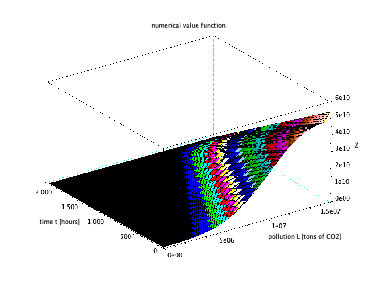
Figure 7 shows the optimal pollution trajectories. We see that the contracts reduce the increment in the pollution levels by more than thirty percent (without regulation the increment is almost 10000000 tons of and with regulation the increment is around 6500000 tons of ).
 |
 |
The optimal production and flow trajectories are shown in Figure 8. The production asked to each firm is piece-wise constant, as well as the flows through the line, and we identify three periods of time in which we describe the actions of the providers. In the first period, the node in the Center is asked to produce exactly MWh, which it does by using only the solar technology and therefore it does not pollute nor incur in any cost. Since this amount does not cover the local demand, the remaining of the demand in the Center is provided by the nodes in the North and the South. In these nodes all the available technologies are used to cover their local demands and what is required by the node in the Center. The node in the North is asked the highest production in the network of MWh. The node in the South produces MWh and receives a flow of MWh from the North. After some time has passed we move into the second period, in which the main change is that the node in the Center is asked to cover most of its local demand, by using all the available technologies and producing MWh. The node in the North contributes with a flow of MWh and no flow is received from the node in the South. The second period occurs when the increase of pollution has been controlled for enough time and it becomes less costly to allow the node in the Center to produce power with the polluting technologies. This is a temporary situation and after some time the node in the Center is asked to act again as in the first period. In the third period, the node in the Center produces exactly MWh by using only the solar technology. The situation here is very similar to the one in the first period, with slight differences in the production of the nodes in the North and the South, as well as the flows they send through the network.
 |
 |
The optimal efforts and the certainty equivalents of the producers are shown in Figure 9. The efforts performed by the firms drop to zero at the end of the contract since, as shown in the example of Section 3.2, when closer to the end of the contract it is too expensive for the ISO to encourage the firms. Prior to the drop, the node in the North, in charge of the highest production, is given incentives to perform full effort and its certainty equivalent increases linearly. The node in the Center receives full incentives during the second period in which it produces with all the technologies, and none during the first and third periods when it produces only with solar technology. The node in the South is the most expensive to encourage (its production is gas-based) and we see that during the third period it is given less incentives than the node in the North which results in an intermediate effort which decreases sooner to zero.
 |
 |
To conclude, let us discuss on the nature of the curves just presented. As mentioned in Section 3.2, constant trajectories are obtained when the spatial derivative of the value function is sufficiently big, which results in the (quadratic) optimisation over the production/flows being attained at the boundaries of some adjusted domain. In the setting with multiple technologies, the objective functional is defined piece-wise and these boundaries depend on the derivative of the value function. The plan of the ISO is dynamically updated and we can identify periods of time during which it remains constant. However, seen as whole trajectories, the optimal production and transmission plans are not constant, which means that the solution to problem of the ISO does not coincide with the one of the simpler problem . Indeed, we have and the solution to problem is attained at the point
To conclude, we perform a sensitivity analysis on the parameter , corresponding to the volatility of the total pollution and thus representing the strength of moral hazard in the problem. We set in tons of and we display in Figure 10 the optimal production and effort of the first provider for different values of . The behaviour of the second and third producers can be deduced from the pictures, by taking into account the discussion above.
 |
 |
We see that the length of the three periods of production is affected by the values of . The smaller the value of this parameter, the shorter is the length of the second period, which is the only period in which the third provider is allowed to pollute. We interpret this by the fact that when decreasing , it is easier to detect moral hazard and to implement a strict policy with almost no pollution. Moreover, when increases, the change from the first to the second period occurs faster and the third configuration becomes predominant. For big values of , in this setting greater than , it is optimal to produce according to the third configuration for the whole life of the contracts. This means that problems and share the same solution. Concerning the optimal efforts, we see that they decrease to zero when the volatility is bigger, since the actions of the providers are harder to detect. In the limit case, when is very large and moral hazard is too strong, the contracts cannot help to control pollution since the providers will exert practically no effort.
References
- Aïd and Biagini [2021] R. Aïd and S. Biagini. Optimal dynamic regulation of carbon emissions market: a variational approach. SSRN preprint 3792384, 2021.
- Aïd et al. [2018] R. Aïd, D. Possamaï, and N. Touzi. Optimal electricity demand response contracting with responsiveness incentives. ArXiv preprint arXiv:1810.09063, 2018.
- Alasseur et al. [2020] C. Alasseur, I. Ekeland, R. Élie, N. Hernández Santibáñez, and D. Possamaï. An adverse selection approach to power pricing. SIAM Journal on Control and Optimization, 58(2):686–713, 2020.
- Aliprantis and Border [2006] C.D. Aliprantis and K. Border. Infinite dimensional analysis: a hitchhiker’s guide. Springer–Verlag Berlin Heidelberg, 3rd edition, 2006.
- Athanassoglou [2010] S. Athanassoglou. Dynamic nonpoint-source pollution control policy: ambient transfers and uncertainty. Journal of Economic Dynamics and Control, 34(12):2494–2509, 2010.
- Bonnans et al. [2004] J.-F. Bonnans, É. Ottenwaelter, and H. Zidani. A fast algorithm for the two dimensional HJB equation of stochastic control. ESAIM: Mathematical Modelling and Numerical Analysis–Modélisation Mathématique et Analyse Numérique, 38(4):723–735, 2004.
- Bontems and Thomas [2006] P. Bontems and A. Thomas. Regulating nitrogen pollution with risk averse farmers under hidden information and moral hazard. American Journal of agricultural economics, 88(1):57–72, 2006.
- Borenstein et al. [2000] S. Borenstein, J. Bushnell, and S. Stoft. The competitive effects of transmission capacity in a deregulated electricity industry. The RAND Journal of Economics, 31(2):294–325, 2000.
- Borodin and Salminen [2002] A.N. Borodin and P. Salminen. Handbook of Brownian motion—facts and formulae. Probability and its applications. Birkhäuser Basel, 2nd edition, 2002.
- Bouchard et al. [2016] B. Bouchard, D. Possamaï, and X. Tan. A general Doob–Meyer–Mertens decomposition for -supermartingale systems. Electronic Journal of Probability, 21(36):1–21, 2016.
- Campbell et al. [2021] S. Campbell, Y. Chen, A. Shrivats, and S. Jaimungal. Deep learning for principal-agent mean field games. arXiv preprint arXiv:2110.01127, 2021.
- Chambers and Quiggin [1996] R. Chambers and J. Quiggin. Non-point-source pollution regulation as a multi-task principal-agent problem. Journal of Public Economics, 59(1):95–116, 1996.
- Cvitanić et al. [2018] J. Cvitanić, D. Possamaï, and N. Touzi. Dynamic programming approach to principal–agent problems. Finance and Stochastics, 22(1):1–37, 2018.
- Dellacherie and Lenglart [1981] C. Dellacherie and É. Lenglart. Sur des problèmes de régularisation, de recollement et d’interpolation en théorie des martingales. Séminaire de probabilités de Strasbourg, XV:328–346, 1981.
- El Karoui and Tan [2013] N. El Karoui and X. Tan. Capacities, measurable selection and dynamic programming part II: application in stochastic control problems. ArXiv preprint arXiv:1310.3364, 2013.
- El Karoui et al. [1997] N. El Karoui, S. Peng, and M.-C. Quenez. Backward stochastic differential equations in finance. Mathematical Finance, 7(1):1–71, 1997.
- Élie and Possamaï [2019] R. Élie and D. Possamaï. Contracting theory with competitive interacting agents. SIAM Journal on Control and Optimization, 57(2):1157–1188, 2019.
- Élie et al. [2021] R. Élie, E. Hubert, T. Mastrolia, and D. Possamaï. Mean-field moral hazard for optimal energy demand response management. Mathematical Finance, 31(1):399–473, 2021.
- Escobar and Jofré [2010] J.F. Escobar and A. Jofré. Monopolistic competition in electricity networks with resistance losses. Economic Theory, 44(1):101–121, 2010.
- Holmström [1982] B. Holmström. Moral hazard in teams. The Bell Journal of Economics, 13(2):324–340, 1982.
- Holmström and Milgrom [1987] B. Holmström and P. Milgrom. Aggregation and linearity in the provision of intertemporal incentives. Econometrica, 55(2):303–328, 1987.
- Hubert [2020] E. Hubert. Continuous-time incentives in hierarchies. arXiv preprint arXiv:2007.10758, 2020.
- Jacod and Shiryaev [2003] J. Jacod and A.N. Shiryaev. Limit theorems for stochastic processes, volume 288 of Grundlehren der mathematischen Wissenschaften. Springer–Verlag Berlin Heidelberg, 2003.
- Jaimungal et al. [2021] S. Jaimungal, A. Shrivats, and D. Firoozi. A mean-field game approach to equilibrium pricing in renewable energy certificate markets. In 2021 Joint Mathematics Meetings (JMM). AMS, 2021.
- La Nauze and Mezzetti [2019] A. La Nauze and C. Mezzetti. Dynamic incentive regulation of diffuse pollution. Journal of Environmental Economics and Management, 93:101–124, 2019.
- Ma and Zhang [2002] J. Ma and J. Zhang. Representation theorems for backward stochastic differential equations. The Annals of Applied Probability, 12(4):1390–1418, 2002.
- Milgrom and Segal [2002] P. Milgrom and I. Segal. Envelope theorems for arbitrary choice sets. Econometrica, 70(2):583–601, 2002.
Appendix A The model
We start by listing the properties that the functions in our model satisfy.
Assumption A.1.
For every we assume
the function is continuous and increasing;
the function is continuous and increasing;
the function is continuous, increasing and strictly convex;
the function is continuously differentiable with quadratic growth, that is, there exists such that for every .
We define also the following constants that will be used in some of the proofs
| (A.1) |
We present now the weak formulation of the problem. We place ourselves in a probability space , representing the randomness in the weather conditions that cannot be controlled. The noise of the model will be given by a one-dimensional standard Brownian motion and the volatility . Let us define the driftless Brownian motion
We denote by , the filtration generated by , completed under the measure . Each producer , has a set of actions , a closed interval, to reduce its own pollution. We denote by the space of controls of producer , that is if it is an -valued, -predictable process. We define the set of joint actions and for a joint effort the probability measure
Notice that since is bounded, and by Novikov’s condition, the stochastic exponential is indeed a true martingale. We have thus, by Girsanov’s theorem, that is a –Brownian motion and the pollution process has the desired dynamics
Finally, for , we define the set of actions of the other producers .
Remark A.2.
As the reader may have noted, both and depend on the production plan. To ease the notation, specially when solving the problem of the providers for whom is fixed, we refrain from adding an additional index to the probability measures and their Brownian motions.
Appendix B Reduction of the class of contracts
B.1 BSDE characterisation of Nash equilibria
In this section, for any admissible contract offered by the ISO, we characterise the set of Nash equilibria through the solutions to a multidimensional BSDE. We start with an auxiliary result. All the proofs are deferred to Section B.2.
Lemma B.1.
For every , the correspondence given by
| (B.1) |
is single-valued and continuous.
Suppose a contract is given. Based on the previous lemma, we introduce the following -dimensional BSDE
| (B.2) |
where the vector function is defined by
| (B.3) |
We define now the notion of solution to the previous BSDE.
Definition B.2.
The space consists in the -valued predictable processes satisfying
Definition B.3.
Before presenting the main result of the section, we need to introduce a family of processes that will be used to reformulate the class of admissible remunerations, as we show below. For and , we define the process through the following SDE
We define finally the following class of processes, using the notation and with the set of stopping times with values in
| (B.4) |
Remark B.4.
The definition of the class is based on the production plan fixed at beginning of this section. However, it is easy to see that the class is independent of the contract due to the multiplicative property of the function and the boundedness of the plan . For this reason we do not index the class on the underlying contract.
The following proposition, similar to the result established in [17], extends the link between principal–agent problems and BSDEs. It is well-known that in the case of a single agent, his problem can be solved by looking at a one-dimensional BSDE. In our setting with agents, we need to consider the -dimensional BSDE defined above.
Proposition B.5.
The previous proposition allows us to reformulate the problem of the ISO (2.5) as a standard stochastic control problem. Indeed, we can represent the admissible remunerations as the terminal values of processes of the form . Therefore, we have the equality
| (B.6) |
which leads to the reformulation of problem (2.7), stated in Theorem 2.4. The controlled process allows to tackle the problem of the ISO by following the dynamic programming approach developed in [13]. It plays the same role as the continuation utility process introduced in [sannikov2008continuous], with the difference that in our model it represents the certainty equivalent of the producers. The last result of this section illustrates this point and states that when a contract having the form (B.6) is offered, the unique Nash equilibrium is given by the process (B.5).
Proposition B.6.
For , consider the contract with . Then the joint effort , given by (B.5), is the unique element in and .
B.2 Proofs
Proof of Lemma B.1.
Since the set is compact and the maps and are continuous, the map
has a minimiser over . The uniqueness of the minimiser follows from the strict convexity of . From the maximum Theorem (see for instance [4, Theorem 17.31]) the function is continuous. ∎
Proof of Proposition B.5.
(i) Let be a Nash equilibrium for the contract . Then for each player the action maximises his expected utility, given the actions of the others
We fix and define the following family of random variables, for
Let us discuss the integrability of this family, which is inherited from the integrability of because the processes and are bounded. From the definition of the set , it is clear that the family , with
is directed upwards. Therefore, there exists a sequence in such that is non-decreasing and . From the monotone convergence theorem we have for every
Take such that , then by Hölder’s inequality and since the density measures have moments of any order we have for every and
where denotes , , and are defined in (A.1), and are the Hölder’s conjugates of and respectively. It follows that
| (B.7) |
We have next the following dynamic programming principle (see for instance [15, Theorem 3.4])99 9 The assumptions of the theorem are satisfied by the continuity of all the functions in our model (see [15, Remark 3.10])., for any such that it holds –a.s.
Then, for every the family is a --supermartingale1010 10 The family is integrable since and are bounded and Equation B.7 holds. system (see [10, Section 3.3] or [14, Definition 10]). From [14, Theorem 15], the family of random variables can be aggregated in a unique -optional process which satisfies
Notice that the value at time of this process coincides with the value function of the agent. Define next, for every , the following process which is a uniformly integrable -supermartingale1111 11 Again, integrability follows from (B.7) and the fact that processes and being bounded. and whose value at time is independent of
Then we have, for any
and it follows that the process is a uniformly integrable -martingale. Since the filtration satisfies the usual conditions, we consider from now on a càdlàg -modification of this process.
From the multiplicative decomposition of negative martingales (see for instance [yoeurp1976decomposition, Equation (8)]) and the martingale representation theorem1212 12 Notice that satisfies the martingale representation property, due to Theorem III.5.24 in [23]., there exists a predictable process such that
By applying Itô’s formula and using the definition of , we obtain that
Finally, defining , , and applying Itô’s formula we have that the pair is a solution to BSDE (B.2). Note also that because , with and .
To conclude, we show that satisfies Condition (B.5). Notice that from definition, for every we have
Since is a (negative) -supermartingale, we conclude that for every we have –a.e. on
which implies (B.5).
For the second part of the proof, let be a solution to BSDE (B.2) such that . Define the process , –a.e. on , by
Next, fix any firm and define for any effort the process
which is a -integrable process of class (D). Indeed, let be such as in (B.4) and notice that , with . Then we have, for every
where we denoted , and is the Hölder’s conjugate of . It follows then that
By Itô’s formula, we have
It follows then that that the process is a -local supermartingale1313 13 It is the stochastic exponential of a continuous semimartingale. of class (D), hence a supermartingale, whose value at time is independent of . By the same argument, we have that is a -martingale, so that
which means the action is the best-reaction for producer , given the action of the others .
∎
Proof of Proposition B.6.
It follows from the proof of Proposition B.5, since the pair is a solution to BSDE (B.2), with . It is also proved that for every . This implies that is a Nash equilibrium and . Moreover, equality is attained only at the control because of the uniqueness of the minimiser in (B.1).
∎
Appendix C Value function of the ISO
Proof of Proposition 2.8.
Note that, for any , the dependence of the objective function on the process is only through the sum of the initial values, that is the coordinates of . By plugging into (2.9), it readily follows then
∎
In the following, we list a series of propositions which will result in Theorem 2.9.
Proposition C.1.
There exists a unique viscosity solution to the HJB equation (2.11) which has at most polynomial growth at infinity. Such solution is continuously differentiable in the space variable, with bounded derivative.
Proof of Proposition C.1.
We start with the uniqueness of such solutions. Define by
We have , with and defined in (A.1). Thus has polynomial growth, and
where is defined in (A.1). Therefore, Assumption (A2) from Pardoux and Râ˙ 2014 [28] is satisfied and the uniqueness of viscosity solutions to (2.11) with polynomial growth follows from [28, Theorem 6.106].
For the existence, we start by proving that is continuously differentiable in , with bounded derivative. Let us denote by the correspondence of optimisers in , as follows
Notice that the optimisation over each can be reduced to a compact set since the objective function is the sum of a bounded and a quadratic function, namely we have where , and are defined in (A.1). Since the correspondence is continuous and compact-valued, it follows from the maximum Theorem (see [4, Theorem 17.31]) that has nonempty compact values and it is upper-hemicontinuous. By Milgrom and Segal 2002 [27, Theorem 2] we have that is absolutely continuous in and we have, for any selection
Since the maps and are uniformly continuous over and respectively, and is upper-hemicontinuous, it follows that is continuous and bounded.
By the previous point, and the fact that the terminal condition in (2.11) is null, we have that the assumptions in Ma and Zhang 2002 [26, Theorem 3.1] as well as their Assumption (A1) are satisfied. It follows that the function , where is the adapted solution to the FBSDE
is a viscosity solution to the PDE. Moreover, exists for every and is continuous. By [26, Corollary 3.2], has polynomial growth at infinity and is bounded. ∎
To make a link between the viscosity solution given by the previous proposition and the value of problem (2.10), we define the value function of the ISO starting from any
| (C.1) |
where is the solution to
Notice that by definition we have the equality , for the value of problem (2.10).
Proposition C.2.
Proof of Proposition C.2.
Since is an infimum, it has an upper bound given by choosing the controls and , where is an arbitrary element of . We have therefore
From [pham2009continuous, Theorem 1.3.15], we have for every , with a constant . This implies that for some
It is clear that is bounded by below so we conclude that has quadratic growth. The fact that is a viscosity solution to the PDE (2.11) is standard in stochastic control. For instance, we can use pham2009continuous [pham2009continuous, Propositions 4.3.1 and 4.3.2], since the function is finite-valued. To conclude, from the uniqueness of viscosity solutions to equation (2.11) we obtain that must coincide with the function in Proposition C.1. Hence, exists and it is bounded. ∎
We turn now our attention to the optimal controls in problem (2.10). Let us denote by the correspondence of optimisers in , for given , that is
Lemma C.3.
The correspondence has nonempty compact values and it is upper-hemicontinuous.
Proof of Lemma C.3.
The proof is identical to part in the proof of Proposition C.1. The optimisation over each can be reduced to a compact set, namely we have From the maximum Theorem [4, Theorem 17.31], has nonempty compact values and it is upper-hemicontinuous. ∎
We can finally prove Theorem 2.9 as a direct consequence of the results in this section.
Proof of Theorem 2.9.
First, the control . Indeed, from the proof of Lemma C.3 we have that is bounded which implies that . Second, since the controls attain the minimum in the Hamiltonian function , they are the optimal controls in the reformulated problem of the ISO.
It follows from Theorem 2.4, that the optimal remuneration is given by . ∎
Appendix D Simpler problem for the ISO
Proof of Proposition 3.2.
We have deduced that and , where is the adapted solution to the FBSDE
with defined by
As in the proof of Proposition C.1, we check that
and for every
with , , , . By restricting the supremum over each to a compact set, as in the proof of Lemma C.3, and by the uniform continuity of all the maps, it follows that as . Then, the hypothesis in [16, Proposition 2.4] are satisfied so we conclude that is continuous. The existence of a minimizer for problem (3.1) holds because is compact.
∎
Proof of Proposition 3.3.
Under the given assumptions, the optimal efforts for the providers are given by
Optimising over , we see that the values for which is outside of are not optimal so we can compute the infimum in directly by replacing . Let and , then
We have the optimal and, recalling , we get
| (D.1) | ||||
Assume for a while that the solution is such that , so then the PDE becomes
with
Let , then satisfies the PDE (provided that is bounded)
Therefore we have from the Feynman–Kac formula under the measure such that Then we have
with , and with . Then we have from the result 2.1.8.3 (page 262) in Borodin and Salminen 2002 [9]
Notice that , so then due to our assumptions. Indeed, we can also compute the value function of the ISO
Since we found a solution to PDE (3.5) with polynomial growth, we know from Theorem 3.1 that we have the value of the problem with fixed plan by . It follows that the optimal process and the optimal efforts are
Finally, we see that the optimal contract is given by
where
∎