Application of canonical augmentation to the atomic substitution problem

SHRY is implemented in Python 3, and uses the CIF format as the standard for both reading and writing the reference and generated sets of substituted structures. Unlike other packages, SHRY is purely implemented in python, and therefore, it can be integrated into another python program, in addition to using it as a stand-alone program without any complicated compilation procedures. Structure abstractions, manipulations, and symmetry analysis leverages the feature sets have been reported in Pymatgen Ong et al. 2013 and spglib Togo and Tanaka 2018. The key point for the implementation is identifying and avoiding, among all possible permutations, multiple instances of symmetrically identical structures. The implementation of a variant of the canonical augmentation McKay 1998 algorithm is unique to SHRY  which allows symmetrically unique structures corresponding to the specified substitute concentration to be recursively generated from the unique structures. Furthermore, the entire set of unique structures for all concentrations can be simultaneously obtained, which is valuable in the study of increasingly complex alloys. When the growth in the number of symmetrically unique structures becomes undesirable, SHRY also allows the random picking of structures up to a user-specified number. Polya’s enumeration theoremPólya 1937; Polya and Read 2012 provides the expected number for the irreducible structures to aid in this picking.

The redundancy of atomic substitutions is attributed to the existence of symmetries in a crystal. Indeed, an atom on a high-symmetric site (i. e. , Wyckoff position Brock et al. 2016) is related to other atoms on the same Wyckoff position via the symmetry operations of the crystal. Thus, one atomic substitution pattern is often equivalent to others from the view point of crystallographic symmetry. SHRY implements a very efficient technique to avoid the redundancy in this search.

Before explaining the algorithm implemented in SHRY  we introduce a few notations and definitions that are used throughout this paper: Given a set $\Omega$, we denote with $\mathrm{Aut}(\Omega)$ the set of bijections $\Omega\rightarrow\Omega$. Let $G$ be a group acting on $\Omega$, i. e. , $G$ has a group homomorphism

called action. We use the notation $g\cdot X$ for $g\in G$ and $X\in\Omega$ for $\phi(g)(X)$. In this setting, the orbit of $X$ is defined as the set

and the orbit space $\Omega/G$ is the set of all distinct orbits, which is a partition of $\Omega$. The cardinality of $\Omega/G$ can be computed using Polya’s theorem Pólya 1937; Polya and Read 2012(sometimes called, Cauchy-Frobenius Lemma, see Ref. 34). Furthermore, given two elements $X$ and $Y$ in $\Omega$, the set $\mathrm{Iso}(X,Y)$ is defined as $\mathrm{Iso}(X,Y)=\{g\in G\ |\ g\cdot X=Y\}$ and, when $X=Y$, we shall use the notation $\mathrm{Aut}(X)=\mathrm{Iso}(X,X)$. Note that $\mathrm{Aut}(X)$ is a subgroup of $G$. We will say that two elements are indistinguishable if $\mathrm{Iso}(X,Y)\neq\emptyset$, i. e. if $X$ and $Y$ belong to the same orbit in $\Omega/G$. An important role in this paper is played by certain functions on $\Omega$ whose value is constant over points in the same orbit: given a set $\Gamma$, a function $f:\Omega\rightarrow\Gamma$ is invariant for the action of $G$ if and only if

which means $f$ can descend to a well-defined function $\tilde{f}:\Omega/G\rightarrow\Gamma$, $\tilde{f}(GX)=f(X)$.

We consider a very simple case—the problem of coloring the 8 vertices of a cube with two colors, as shown in Fig 1—to explain the main idea of SHRY. We color white vertices with red step-by-step until three of them become red. This is essentially equivalent to the substitution in which three out of eight atoms on a Wyckoff position are substituted with another element (e.g., see Fig. 2. Ce₈Pd₂₄Sb $\rightarrow$ (Ce₅,La₃)Pd₂₄Sb, where Ce and La atoms are on the 8$g$ Wyckoff position and the space group is 221-$Pm\bar{\rm 3}m$). We discuss atomic substitutions as if there were no translation symmetry, as in the cube example (i. e. , not the space group but the point group); however, our considerations can be extended easily to periodic systems.

The main example of the group action relevant in this work is as follows: let us assign indices $I=(1,2,...8)$ to the vertices of a cube. Let $G$ denote the group composed of symmetry operations of the cube, which is also referred to as the point group in chemistry (i. e. , $O_{h}$ in the Schoenflies notation). Once we define a one-to-one correspondence between vertices and indices, the action of $g\in G$ on $I$ can be represented as a permutation operation such as $\begin{pmatrix}1&2&3&4&5&6&7&8\\ 8&7&3&4&5&6&2&1\\ \end{pmatrix}\equiv(1,8)(2,7),$ and $\begin{pmatrix}1&2&3&4&5&6&7&8\\ 7&8&5&6&3&4&1&2\\ \end{pmatrix}\equiv(1,7)(2,8)(3,5)(4,6)$. Each symmetry of the cube corresponds to one of the permutations. For example, the permutation operation (1,8)(2,7) mirrors the cube with respect to the plane containing the vertices {3,4,5,6} and (1,7)(2,8)(3,5)(4,6) inverts all the cubes. The cube has 48 automorphisms, i. e. , the order of $O_{h}$ is 48 as there are 48 symmetry operations that do not change the cube. Therefore, in SHRY  all symmetry operations of a crystal structure associated with the space group are held as a set of permutations of atom indices.

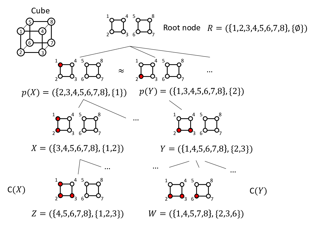
Let $X$ be an ordered partition of $I$, $X=(V_{1},V_{2})$, $V_{1}\subset I$, $V_{2}\subset I$, and $V_{1}\cup V_{2}=I,V_{1}\cap V_{2}=\emptyset$. The sets $V_{1}$ and $V_{2}$ are color classes composed of vertex indices. For instance, $X=\{\{3,4,5,6,7,8\},\{1,2\}\}$ refers to the cube whose first and second vertices are colored by red while the others are white ($X$ in Fig. 1). We denote with $\Omega$ the finite set composed of all ordered partitions of $I$. The action of $G$ on $I$ can be easily extended to $\Omega$ as follows: given $g\in G$ and $X\in\Omega$, we define $g\cdot X$ as

which is well-defined because $g$ is a permutation and $\{V_{1},V_{2}\}$ is a partition of $I$.

The set $\Omega$ of all possible ordered partitions of $I$ (i. e. , coloring patterns of $I$) is a key set for our analysis. The elements of $\Omega$ can be generated recursively using a rooted tree structure $(T_{I},R)$ as follows: root $R$ is given by the ordered partition $(I,\emptyset)$ because, for the recursion step, the set of children of $X$, denoted with $C(X)$, is defined as $C(X)=\{(V_{1}\setminus\{i\},V_{2}\cup\{i\}):i\in V_{1}\}$ given a node $X=(V_{1},V_{2})\in T_{I}$. There is an urgent need to see that the depth of $T_{I}$ is exactly $I$. Indeed, we have that the set of nodes on $T_{I}$ is $\Omega$; given this identification, we denote a set of non-root nodes of $T_{I}$ by $\Omega_{nr}$. Moreover, we can just truncate the tree $T_{I}$ at depth $|V_{2}|$ to consider only those ordered partitions where $V_{2}$ has a fixed number of elements. For a node $X\in T_{I}$, we denote the parent node of $X$ by $p(X)$. Fig 1 presents the pictorial representation of these definitions.

Given this setting, we summarize the main goal to be achieved by SHRY as follows: efficiently generate all indistinguishable elements of $\Omega$ by partially traversing the tree $T_{I}$. That is, we want to extract a representative for each orbit $O\in\Omega/G$; in this way, we can obtain a fast enumeration of all indistinguishable atomic substitution patterns of a given structure.

Although it would certainly lead to a correct algorithm, we cannot hope to achieve our goal through the exhaustive traversal of the search tree $T_{I}$ because the number of elements of $\Omega$, i. e.  all possible substitution patterns of a given structure, is of the order of trillions in many cases. Indeed, a straightforward solution to the problem would be to generate all configurations row-by-row, as described by the search tree in Fig. 1, and then to maintain a record of the complete configurations (i. e.   elements of the set of leaves of the tree $T_{I}$) encountered, and output a complete configuration only if it is not isomorphic to a complete configuration appearing on record until the number of pooled configurations equals the cardinality of $\Omega/G$ obtained from Polya’s theorem Kaski and Östergård 2005. Clearly, this solution is correct and works for the simple cube as shown in Fig. 1; however, for such a solution, it would not be particularly efficient and unfeasible in the actual crystal structure substitution problem, regardless of the implementation, because the total number of patterns often exceeds several billions. Further, the search tree in Fig. 1 indicates that the same isomorphism class of atomic substitution pattern is encountered multiple times in the traversal; this implies that useless computations are often performed, i. e. checking whether the current configuration lies in an orbit that has not been encountered yet. The need of performing all such checks worsens the efficiency of the algorithm, because in many cases, we check if $X\cong Y$ is a computationally demanding operation.

Efficiency issues outlined above can be addressed using the isomorph rejection technique. The term isomorph rejection was introduced in Ref. 39 for techniques that can eliminate redundancy in problems requiring exhaustive search. The main idea of isomorph rejection is explained as follows Kaski and Östergård 2005: if isomorphic nodes are assumed to have isomorphic children (assumption fulfilled for $T_{I}$), then, in the traversal of the search tree, we can prune those subtrees whose root belongs to an isomorphism class already encountered; clearly, traversing only the non-pruned subtrees suffices for isomorph-free exhaustive generation. A straightforward implementation of the isomorph rejection involves keeping a global record $\mathcal{R}$ of the objects seen so far during the traversal of the search tree. Whenever an object $X$ is encountered, it is tested for isomorphism against the recorded objects in $\mathcal{R}$. If $X$ is isomorphic to a recorded object, then the subtree rooted at $X$ is pruned as redundant. This approach is presented in Algorithm 1.

Although the isomorph rejection approach is more efficient than the naive exhaustive generation, the algorithm is not practical for our complex problem because of two reasons: first, a clear difficulty of this implementation is that it requires storing the set $\mathcal{R}$ of the non-isomorphic objects encountered. When the number of nonisomorphic partial objects is large, the available memory (or storage) space can quickly run out. Second, there is still a need to perform the check whether two nodes are isomorphic too many times.

These subtleties can be overcome using a technique called canonical augmentation, implemented in SHRY  which is a refinement of isomorph rejection. A detailed explanation of this canonical augmentation technique is provided in Chapter 4.3 of Ref. 28. In brief, the key of the canonical augmentation algorithm is a relationship between a node $X$ and its parent $p(X)$. To this end, we extend the definition of the isomorphism to the pair of objects: given $X,Y,W,Z\in\Omega$, $(X,Z)$ is isomorphic to $(Y,W)$, which is denoted as $(X,Z)\cong(Y,W)$ if and only if there exists a $g\in G$ such that $g\cdot X=Y$ and $g\cdot Z=W$.

A key feature of the canonical augmentation algorithm is the existence of certain functions that map nodes to other nodes. Consider a function $m:\Omega_{nr}\rightarrow\Omega$ such that, for all $X,Y\in\Omega_{nr}$ $(X,m(X))\cong(Y,m(Y))$, if and only if $X\cong Y$. The function $m$ is called a canonical parent function and the pair $(X,m(X))$ is called the canonical augmentation of $X$. Using such a function $m$, provided that the pair $(\Omega,m)$ satisfies certain assumptions, one can devise Algorithm 2 so that it returns exactly one element for each orbit of the action of $G$ on $\Omega$. The assumptions required to ensure that Algorithm 2 returns the desired output are

The key observation on the pair $(\Omega,m)$ is as follows: assume that $Z$ and $W$ are isomorphic nodes encountered in the tree traversal. Furthermore, assume that both nodes are generated by canonical augmentation. It then follows that

which implies $p(Z)\cong p(W)$. Now, if isomorph rejection has already been performed on parent nodes, $Z$ and $W$ are siblings. Moreover, from the above chain of pair isomorphisms, we get that $(Z,X)\cong(W,X)$, where $X=p(Z)=p(W)$ implies that $a\cdot Z=W$ for some $a\in\mathrm{Aut}(X)$. Thus, we conclude that any two isomorphic nodes $Z$ and $W$ generated by canonical augmentation must be related by an automorphism of their common parent node, i. e. , $X$. Thus, it follows that one has to perform isomorph rejection only among siblings when traversing a search tree based on the automorphisms of $X$; this drastically decreases the computational cost compared with the simple isomorphic rejection technique. Furthermore, no objects need to be stored in memory for isomorph rejection. Moreover, the decision whether to accept or reject a node can be made locally based on a procedure that determines whether the child node $X$ is generated by canonical augmentation. In addition, the search can be efficiently parallelized because disjoint subtrees can be searched independently of each other.

The key to implementation is defining function $m$ that satisfies the relation $(X,m(X))\cong(Y,m(Y))$ and Assumptions 1 and 2. We now explain how to define such a function for the atomic substitution pattern problem, which SHRY solves. First, the search tree $T_{I}$ fulfills Assumption 1. As such, we are left to finding $m$ such that $m$ is a canonical parent function and Assumption 2 is satisfied. We define a function $W$ that, given in input a set of non-root nodes, it returns the node that is the smallest with respect to the lexicographic order. We define the function

where argmin works within the lexicographic order, and the notation $\mathcal{P}(-)$ stands for the power set operation. Using $L$, we can define a canonical labeling map for the action of $G$ on $\Omega$, i. e. a function $\kappa:\Omega\rightarrow G$ such that, for all $g\in G$ and $X\in\Omega$, the following holds.

To define $\kappa$, we proceed as follows: for $X\in\Omega$, let $g_{X}\in G$ such that $g_{X}X=L(GX)$. It is easy to see that, in our case, at least one such $g_{X}$ always exists, for all $X\in\Omega$. Then, we define

The fact that $\kappa$ is indeed a canonical labeling map is an immediate consequence of the equality

that holds for all $g\in G$ and $X\in\Omega$, from the very definition of the orbit. We need one last definition to define the canonical parent map: for the nonroot node $X$, we define the set of subobjects of $X$, denoted with $S(X)$, as

The set $S(X)$ can also be considered as the set of all possible parents of $X$ in the search tree $T_{I}$. Finally, we define the function $m$ as

The above construction of the map $m$ is an instance of a procedure, outlined in Chapter 4.2.3 of Ref. 28, to construct a canonical parent function that satisfies Assumption 2 starting from canonical labeling; the procedure reads

1. a).

   Compute the canonical labeling $\kappa(Z)\in G$ and the canonical form $\hat{Z}=\kappa(Z)Z$ for $Z$;

2. b).

   Select a sub-object ${\hat{Z}}_{0}\in S(\hat{Z})$ such that the selection depends only on the canonical form $\hat{Z}$ and not on $Z$ and that the following equation holds: $\hat{Z}=\hat{W}$ and ${\hat{Z}}_{0}={\hat{W}}_{0}$ for any two isomorphic objects, $Z,W\in\Omega_{nr}$;

3. c).

   Define $m(Z)\coloneqq\kappa(Z)^{-1}{\hat{Z}}_{0}$.

Our construction of $m$ follows the above steps; therefore, Assumptions 1 and 2 are fulfilled for $m$. Thus, Algorithm 2 allows us to extract representative orbits, i. e. , the set of unique atomic substitution patterns, in a very efficient manner.

The canonical augmentation algorithm can be further improved using subobject invariants, as defined in Chapter 3.3.4 Ref. 28, which allows us to avoid the computationally expensive calculation of the object $m(X)$. This is a great advantage of the canonical augmentation algorithm over the orderly generation that needs to check the canonicity of a structure every time Kaski and Östergård 2005. Indeed, in Algorithm 2, we are essentially only interested in testing whether

holds for a nonroot node $Z\in\Omega_{nr}$ encountered in the search. It suffices to check whether $m(Z)$ and $p(Z)$ are in the same orbit of the action of ${\rm{Aut}}(Z)$ on the set of subobjects $S(Z)$ (it is necessary to check if the action of $G$ on $\Omega$ induces an action of $\mathrm{Aut}(Z)$ on $S(Z)$) to check whether the isomorphism Eq. (5) holds. This observation can often be exploited to gain efficiency: indeed, assume that one can define a function $\phi:\Omega_{nr}\rightarrow\Gamma$, where $\Gamma$ is a poset such that for all $Z\in\Omega_{nr}$, it induces an invariant map

and the minimum of $\tilde{\phi}$ on $S(Z)/\mathrm{Aut}(Z)$ is unique. Such a minimum is denoted as $\gamma_{Z}$. Within this framework, we replace the definition of $m$ given in Eq. (4) with

With this definition of $m$, it suffices to check whether

to verify that $m(X)$ and $p(X)$ are in the same orbit for the action of $\mathrm{Aut}(X)$ on $S(X)$. Indeed, in this case, the property of $\tilde{\phi}$ guarantees that there exists $g\in\mathrm{Aut}(X)$ such that $g\cdot p(X)=m(X)$. For our case, we consider the function $T:\Omega_{nr}\rightarrow\mathbb{R}^{2}$, where $T(Z)$ represents a tuple of the sums of the distance matrices, $T(Z)=(D(V);V\in Z$), where $D(V)=\sum_{i,j}d_{i,j};i,j\in V$, and $d_{i,j}$ is the Euclidean distance between vertices (atoms) $i$ and $j$ in the cube (in a crystal), and the partial order on $\mathbb{R}^{2}$ is the lexicographic one. One can select a different function $D(V)$ as far as it is invariant with respect to symmetry operations such as the determinant, i. e. , $D(V)=\det(d_{i,j});i,j\in V$. Only one between $D(V_{1})$ and $D(V_{2})$ is sufficient to define the invariant in the simple case; however, we use the given definition as it generalizes naturally when substituting atoms in a Wyckoff position with more than two elements, or when targeting more than the Wyckoff positions. Indeed, function $T$ is invariant with respect to the action of $G$ on $\Omega$. Therefore, for each $Z\in\Omega$, $T$ descends to a map $\tilde{T}:S(Z)/\mathrm{Aut}(Z)\rightarrow\mathbb{R}^{2}$; unfortunately, the minimum of $\tilde{T}$ on $S(Z)/\mathrm{Aut}(Z)$ is not unique; therefore, if we define the canonical augmentation map as per Eq. (7), we cannot straightforwardly follow the above procedure: given two nodes $X$ and $Y$, if $T(X)\neq T(Y)$, $X$ and $Y$ cannot be isomorphic by definition; the vice versa does not hold, i. e. two nodes with the same invariant $T$ may or may not be isomorphic. Thus, given a node $Z$, if $p(Z)$ is the unique subobject in $S(Z)$ which realizes the minimum of $T$, then we must have $p(Z)=m(Z)$; this can be decided by invariant computations only, without ever computing $m(Z)$. Similarly, if $p(Z)$ does not have the maximum invariant value in $S(Z)$, $p(Z)$ and $m(Z)$ must occur in different orbits of $Aut(Z)$ on $S(Z)$. In the case where $p(Z)$ is not the unique subobject in $S(Z)$ with the minimum determinant (i. e. , $S(Z)$ includes two or more objects which realize the minimum of $T$ in $S(Z)$); then, we must proceed with the usual procedure with canonical labeling and explicitly compute $m(Z)$. Several benchmark results of the acceleration are shown in Table 2. The results imply that the use of the distance matrix does not always accelerate the computation. This is because the current implementation, i.e., the sum of distance matrix, is often too simple to distinguish structures belonging to different orbits on a subobject. A more distinguishable subject invariant could certainly accelerate the exhaustive search. This is an interesting future work to fully exploit the advantage of the canonical augmentation algorithm.

The algorithm can be easily extended to replace a single site with three or more elements or to replace two or more sites. We assign sequential indices for the atomic site $I=\{1,2,....N_{\rm atom}\}$, where $N_{\rm atom}$ is the number of atoms in the simulation cell. Then, we define

where $n_{c}(i)$ and $n_{w}$ represent the number of different elements in the $i$-th Wyckoff position, and the number of Wyckoff positions in a crystal, respectively. The same element in different Wyckoff sites are treated as different type of elements. In the multielement and multi-Wyckoff frameworks, an analogue of tree $T_{I}$ can be generated according to the rule: given a node $X$, the set of its children is $C(X)$, which is defined as

for the $j$-th ($j>1$) element in the $i$-th wyckoff position. When the atomic substitution ends for the $j$-th element in the $i$-th Wycoff position, SHRY proceeds with the substitution for the $(j+1)$-th element in the $i$-th Wyckoff position. ¹¹ 1 One can employ a different sequence of the substitution: e.g. when substituting A with B and C (A₈ $\rightarrow$ A₅B₂C₁), substituting A with B’ (=B+C) (i.e., A₈ $\rightarrow$ A₅B’₃) first, then replacing B’ with C (i.e., A₅B’₃ $\rightarrow$ A₅B₂C₁). Similarly, when the atomic substitution ends for the $i$-th Wyckoff position, SHRY proceeds with the substitution for the $(i+1)$-th Wyckoff position. The schematic is shown in Fig. 4. Accordingly, given a node $X$, the set $S(X)$ of subobjects of $X$ is defined with the formula

for the $j$-th ($>1$) element in the $i$-th Wyckoff position. Functions $L$, $K$, and $T$ are extended in a natural manner. Thus, theorems and methods discussed for the single-element, single-Wyckoff case also hold for the multielement and multiWyckoff cases.

Another possible extension of the canonical augmentation algorithm is to the case of periodic systems. This can be achieved by using the space group $\tilde{G}$ instead of the point group ${G}$. A user needs to specify the size of the supercell so that the number of substituted atoms becomes an integer for the desired solid solubility. The space group $\tilde{G}$ is composed of an infinite number of elements of translation symmetry. Therefore, we treat all translation symmetries larger than the lattice vectors of the specified supercell size as the identity transformation.

Coulomb energy is useful for predicting the stability of the proposed structure before performing more expensive ab initio calculations. Since SHRY can provide Pymatgen’s Structure in runtime, a user can filter out less stable structures before saving them to the disk using the corresponding module from Pymatgen or any other tool of choice. We provide an example on how to do this with the distribution.

References

- Kageyama et al. (2018) Kageyama, H.; Hayashi, K.; Maeda, K.; Attfield, J. P.; Hiroi, Z.; Rondinelli, J. M.; Poeppelmeier, K. R. Expanding frontiers in materials chemistry and physics with multiple anions. Nat. Commun. 2018, 9, 1–15.
- Ichibha et al. (2019) Ichibha, T.; Prayogo, G.; Hongo, K.; Maezono, R. A new ab initio modeling scheme for the ion self-diffusion coefficient applied to the -Cu3Sn phase of the CuSn alloy. Phys. Chem. Chem. Phys. 2019, 21, 5158–5164.
- Ichibha et al. (2019) Ichibha, T.; Benali, A.; Hongo, K.; Maezono, R. Ti interstitial flows giving rutile reoxidation process enhancement in (001) surface. Phys. Rev. Materials 2019, 3, 125801.
- Bellaiche and Vanderbilt (2000) Bellaiche, L.; Vanderbilt, D. Virtual crystal approximation revisited: Application to dielectric and piezoelectric properties of perovskites. Phys. Rev. B 2000, 61, 7877–7882.
- Soven (1967) Soven, P. Coherent-Potential Model of Substitutional Disordered Alloys. Phys. Rev. 1967, 156, 809–813.
- Korringa (1947) Korringa, J. On the calculation of the energy of a Bloch wave in a metal. Physica 1947, 13, 392–400.
- Kohn and Rostoker (1954) Kohn, W.; Rostoker, N. Solution of the Schrödinger equation in periodic lattices with an application to metallic lithium. Phys. Rev. 1954, 94, 1111.
- Nakano et al. (2016) Nakano, K.; Hongo, K.; Maezono, R. Phonon dispersions and Fermi surfaces nesting explaining the variety of charge ordering in titanium-oxypnictides superconductors. Sci. Rep. 2016, 6, 29661.
- Nakano et al. (2017) Nakano, K.; Hongo, K.; Maezono, R. Investigation into Structural Phase Transitions in Layered Titanium-Oxypnictides by a Computational Phonon Analysis. Inorg. Chem. 2017, 56, 13732–13740.
- Utimula et al. (2020) Utimula, K.; Hunkao, R.; Yano, M.; Kimoto, H.; Hongo, K.; Kawaguchi, S.; Suwanna, S.; Maezono, R. Machine-Learning Clustering Technique Applied to Powder X-Ray Diffraction Patterns to Distinguish Compositions of ThMn12-Type Alloys. Adv. Theory Simul. 2020, 3, 2000039.
- Wei et al. (1990) Wei, S.-H.; Ferreira, L. G.; Bernard, J. E.; Zunger, A. Electronic properties of random alloys: Special quasirandom structures. Phys. Rev. B 1990, 42, 9622–9649.
- Zunger et al. (1990) Zunger, A.; Wei, S.-H.; Ferreira, L. G.; Bernard, J. E. Special quasirandom structures. Phys. Rev. Lett. 1990, 65, 353–356.
- Seko et al. (2009) Seko, A.; Koyama, Y.; Tanaka, I. Cluster expansion method for multicomponent systems based on optimal selection of structures for density-functional theory calculations. Phys. Rev. B 2009, 80, 165122.
- Yoshio et al. (2021) Yoshio, S.; Hongo, K.; Nakano, K.; Maezono, R. High-Throughput Evaluation of Discharge Profiles of Nickel Substitution in LiNiO2 by Ab Initio Calculations. J. Phys. Chem. C 2021, 125, 14517–14524.
- Freysoldt et al. (2009) Freysoldt, C.; Neugebauer, J.; Van de Walle, C. G. Fully Ab Initio Finite-Size Corrections for Charged-Defect Supercell Calculations. Phys. Rev. Lett. 2009, 102, 016402.
- Rurali and Cartoixà (2009) Rurali, R.; Cartoixà, X. Theory of defects in one-dimensional systems: application to Al-catalyzed Si nanowires. Nano lett. 2009, 9, 975–979.
- Murphy and Hine (2013) Murphy, S. T.; Hine, N. D. M. Anisotropic charge screening and supercell size convergence of defect formation energies. Phys. Rev. B 2013, 87, 094111.
- Kumagai and Oba (2014) Kumagai, Y.; Oba, F. Electrostatics-based finite-size corrections for first-principles point defect calculations. Phys. Rev. B 2014, 89, 195205.
- Utimula et al. (2021) Utimula, K.; Prayogo, G. I.; Nakano, K.; Hongo, K.; Maezono, R. Stochastic Estimations of the Total Number of Classes for a Clustering having Extremely Large Samples to be Included in the Clustering Engine. Adv. Theory Simul. 2021, 4, 2000301.
- Okhotnikov et al. (2016) Okhotnikov, K.; Charpentier, T.; Cadars, S. Supercell program: a combinatorial structure-generation approach for the local-level modeling of atomic substitutions and partial occupancies in crystals. J. Cheminformatics 2016, 8, 1–15.
- (21) Dassault Systèmes BIOVIA, Materials Studio, Version 18.1.0.2017, San Diego: Dassault Systèmes, 2018.
- Hart and Forcade (2008) Hart, G. L. W.; Forcade, R. W. Algorithm for generating derivative structures. Phys. Rev. B 2008, 77, 224115.
- Ong et al. (2013) Ong, S. P.; Richards, W. D.; Jain, A.; Hautier, G.; Kocher, M.; Cholia, S.; Gunter, D.; Chevrier, V. L.; Persson, K. A.; Ceder, G. Python Materials Genomics (pymatgen): A robust, open-source python library for materials analysis. Comput. Mater. Sci. 2013, 68, 314 – 319.
- Mustapha et al. (2013) Mustapha, S.; D’Arco, P.; De La Pierre, M.; Noël, Y.; Ferrabone, M.; Dovesi, R. On the use of symmetry in configurational analysis for the simulation of disordered solids. J. Condens. Matter Phys. 2013, 25, 105401.
- Dovesi et al. (2018) Dovesi, R.; Erba, A.; Orlando, R.; Zicovich-Wilson, C. M.; Civalleri, B.; Maschio, L.; Rérat, M.; Casassa, S.; Baima, J.; Salustro, S.; Kirtman, B. Quantum-mechanical condensed matter simulations with CRYSTAL. Wiley Interdiscip. Rev. Comput. Mol. Sci. 2018, 8, e1360.
- Grau-Crespo et al. (2007) Grau-Crespo, R.; Hamad, S.; Catlow, C. R. A.; De Leeuw, N. Symmetry-adapted configurational modelling of fractional site occupancy in solids. Journal of Physics: Condensed Matter 2007, 19, 256201.
- Read (1978) Read, R. C. Every one a winner or how to avoid isomorphism search when cataloguing combinatorial configurations. Ann. Discrete Math. 1978, 2, 107–120.
- Kaski and Östergård (2005) Kaski, P.; Östergård, P. R. J. Classification Algorithms for Codes and Designs (Algorithms and Computation in Mathematics); Springer-Verlag: Berlin, Heidelberg, 2005.
- Togo and Tanaka (2018) Togo, A.; Tanaka, I. Spglib: a software library for crystal symmetry search. arXiv 1808.01590 2018,
- McKay (1998) McKay, B. D. Isomorph-Free Exhaustive Generation. J. Algorithms 1998, 26, 306 – 324.
- Pólya (1937) Pólya, G. Kombinatorische anzahlbestimmungen für gruppen, graphen und chemische verbindungen. Acta mathematica 1937, 68, 145–254.
- Polya and Read (2012) Polya, G.; Read, R. C. Combinatorial enumeration of groups, graphs, and chemical compounds; Springer Science & Business Media, 2012.
- Brock et al. (2016) Brock, C. P.; Hahn, T.; Wondratschek, H.; Müller, U.; Shmueli, U.; Prince, E.; Authier, A.; Kopskỳ, V.; Litvin, D.; Arnold, E., et al. International tables for crystallography volume A: Space-group symmetry. 2016.
- Kerber (2013) Kerber, A. Applied finite group actions; Springer Science & Business Media, 2013; Vol. 19.
- Gordon and DiSalvo (1996) Gordon, R. A.; DiSalvo, F. J. Crystal structure and magnetic susceptibility of Ce8Pd24Sb. Zeitschrift für Naturforschung B 1996, 51, 52–56.
- Bergerhoff et al. (1983) Bergerhoff, G.; Hundt, R.; Sievers, R.; Brown, I. The inorganic crystal structure data base. J. Chem. Inf. Comput. Sci. 1983, 23, 66–69.
- Hellenbrandt (2004) Hellenbrandt, M. The inorganic crystal structure database (ICSD)―present and future. Crystallogr. Rev. 2004, 10, 17–22.
- Momma and Izumi (2011) Momma, K.; Izumi, F. VESTA 3 for three-dimensional visualization of crystal, volumetric and morphology data. J. Appl. Crystallogr. 2011, 44, 1272–1276.
- Swift (1960) Swift, J. Isomorph rejection in exhaustive search techniques. Combinatorial Analysis. Providence RI, 1960; pp 195–200.
- Gražulis et al. (2009) Gražulis, S.; Chateigner, D.; Downs, R. T.; Yokochi, A. F. T.; Quirós, M.; Lutterotti, L.; Manakova, E.; Butkus, J.; Moeck, P.; Le Bail, A. Crystallography Open Database – an open-access collection of crystal structures. J. Appl. Crystallogr. 2009, 42, 726–729.
- Dovesi et al. (2020) Dovesi, R.; Pascale, F.; Civalleri, B.; Doll, K.; Harrison, N. M.; Bush, I.; D’arco, P.; Noël, Y.; Rérat, M.; Carbonniere, P., et al. The CRYSTAL code, 1976–2020 and beyond, a long story. J. Chem. Phys. 2020, 152, 204111.