Simultaneous best linear invariant prediction of future order statistics for location-scale and scale families and associated optimality properties

Let $\boldsymbol{X}=(X_{1:n},\ldots,X_{r:n})^{\top}_{r\times 1}$ be the available Type-II right censored data from a location-scale family of distributions in (1). Let us then use the following notation: $\alpha_{i}$ for the expected value of the standardized order statistic

with $\boldsymbol{\alpha}=(\alpha_{1},\ldots,\alpha_{r})^{\top}_{r\times 1}$ and $\sigma^{2}\boldsymbol{\Sigma}$ for the variance-covariance matrix of $\boldsymbol{X}$, where $\boldsymbol{\Sigma}$ is the $r\times r$ covariance matrix of $Z_{i:n},i\in\{1,\ldots,r\}$, assumed to be positive definite. In addition, let $\boldsymbol{1}$ denote a column vector $(1,\ldots,1)^{\top}_{r\times 1}$. Using these notations, we then can write

and

Thence, upon minimizing the generalized variance

with respect to $\mu$ and $\sigma$, the BLUEs $(\mu^{*},\sigma^{*})$ of $(\mu,\sigma)$ are obtained as

with

and

being the determinant of the matrix

which is related to the variance-covariance matrix of the BLUEs $(\hat{\mu},\hat{\sigma})$; see Balakrishnan and Cohen, 1991, David and Nagaraja, 2003 and Arnold et al., 1992 for pertinent details.

Using the general framework of best linear unbiased prediction developed by Goldberger, 1962 for generalized linear regression model, a point BLUP of $X_{s:t},\quad r<s\leq n,$ was derived by Kaminsky and Nelson, 1975 as

where $\boldsymbol{\omega}_{s}=(\omega_{1},\ldots,\omega_{r})^{\top}_{r\times 1}$, with $\omega_{i}=\mbox{Cov}(Z_{i:n},Z_{s:n})$. Consequently, the mean squared predictive error is given by

where $c_{11}=\mbox{Var}\{(1-\boldsymbol{\omega}^{\top}_{s}\boldsymbol{\Sigma}^{-1}\boldsymbol{1})\mu^{*}+(\alpha_{s}-\boldsymbol{\omega}^{\top}_{s}\boldsymbol{\Sigma}^{-1}\boldsymbol{\alpha})\sigma^{*}\}/\sigma^{2}$. An alternative expression to (3) of $\tilde{X}_{s:n}$ has been presented recently by Balakrishnan and Bhattacharya, 2021b as

where

with $V_{1}=\boldsymbol{1}^{\top}\boldsymbol{\Sigma}^{-1}\boldsymbol{1}$, $V_{2}=\boldsymbol{\alpha}^{\top}\boldsymbol{\Sigma}^{-1}\boldsymbol{\alpha}$, $V_{3}=\boldsymbol{1}^{\top}\boldsymbol{\Sigma}^{-1}\boldsymbol{\alpha}$, $A_{s}=1-\boldsymbol{1}^{\top}\boldsymbol{\Sigma}^{-1}\boldsymbol{\omega}_{s}$, $B_{s}=\alpha_{s}-\boldsymbol{\alpha}^{\top}\boldsymbol{\Sigma}^{-1}\boldsymbol{\omega}_{s}$, and $\Delta$ as defined earlier in (2).

Proceeding similarly, Balakrishnan and Bhattacharya, 2021a also derived explicit expressions for the joint best linear unbiased predictors $(\tilde{X}_{s:n},\tilde{X}_{t:n})$ of $(X_{s:n},X_{t:n})$, for $r<s<t\leq n$, as

where

with $A_{t}=1-\boldsymbol{1}^{\top}\boldsymbol{\Sigma}^{-1}\boldsymbol{\omega}_{t}$, $B_{t}=\alpha_{t}-\boldsymbol{\alpha}^{\top}\boldsymbol{\Sigma}^{-1}\boldsymbol{\omega}_{t}$ and $\boldsymbol{a}$ defined exactly as in (5). Moreover, the joint MSPE matrix has been given by these authors to be

where

Further, explicit expressions for the simultaneous BLUPs of any $\ell$ future order statistics have been given in Theorem 3 of Balakrishnan and Bhattacharya, 2021b.

The best linear invariant estimators of $(\mu,\sigma)$ were first developed by Mann, 1969, and upon using these results of Mann, 1969, an expression for the BLIP $\hat{X}_{s:n}$ of $X_{s:n},\quad r<s\leq n$ was presented by Kaminsky et al., 1975 as

where $\sigma^{2}c_{12}=\mbox{Cov}(\sigma^{*},\tilde{X}_{s:n}-\boldsymbol{\omega}^{\top}_{s}\boldsymbol{\Sigma}^{-1}\boldsymbol{X})$ and $\sigma^{2}c_{22}=\mbox{Var}(\sigma^{*})$. The corresponding mean squared predictive error is given by

where $\mbox{MSPE}(\tilde{X}_{s:n})$ is as given in (4). In the next section, we first present an alternate expression to (6) for the marginal BLIP of $X_{s:n}$ and its MSPE.

The quantity $\delta$ plays an important role in the relative performance of the BLIP $\hat{X}_{s:n}$ against the BLUP $\tilde{X}_{s:n}$. Let us define the relative efficiency measure

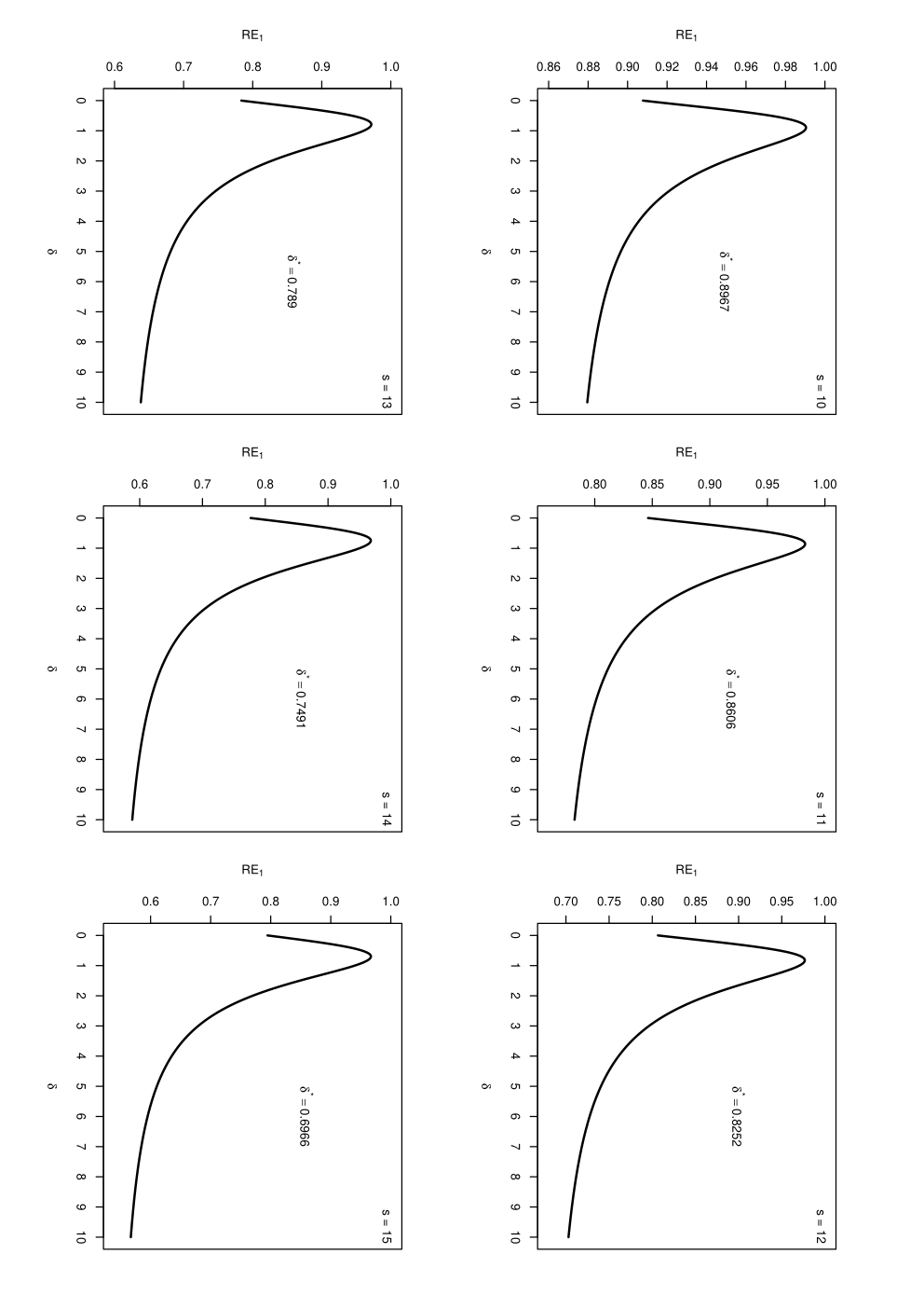
Note that $\mbox{RE}_{1}$ is a continuous function of $\delta$. For example, with $n=15$ and $r=9$, we have plotted RE₁ against $\delta$ in Figure 1 for $s=10,11,12,13,14$ and 15. Note that the range of $\delta$ is $(-\infty,0)\cup(0,\infty)$. However, due to symmetry, we an focus on the interpretation of the behavior of $\mbox{RE}_{1}$ in $(0,\infty)$. Figure 1 shows the unique maximum of $\mbox{RE}_{1}$ is attended at some $\delta^{*}$ which can be found numerically. Note that all $\mbox{RE}_{1}$ are less than 1 indicating that BLIP always possesses less mean squared error than BLUP. When $\delta\rightarrow\delta^{*}$, $\mbox{RE}_{1}$ approaches to its maximum value. Therefore, from a practical point of view, one can measure how well BLIP performs better than BLUP by simply estimating $\delta$, say $\hat{\delta}$, using the BLUEs of $\mu$ and $\sigma$ as $\hat{\delta}=\mu^{*}/\sigma^{*}$. Thus, for values of $\hat{\delta}$ away from $\delta^{*}$, the BLIP will have better performance meaning less mean squared error.

Let us consider an environmental lead contamination data 26, 63, 3, 70, 16, 5, 1, 57, 5, 3, 24, 2, 1, 48 and 3 presented by Bhaumik and Gibbons, 2004. The data were also analyzed by Krishnamoorthy and Hasan, 2018 and showed that a log-normal distribution fits the data well. In our case, we first take the logarithmic transformation of the data. Then, assuming that the first $r=9$ ordered data are observed, we have $\boldsymbol{X}=(0,0,0.693,1.099,1.099,1.099,1.609,$ $1.609,2.773)^{\top}$. Based on $\boldsymbol{X}$, the BLUEs of $(\mu,\sigma)$ are computed as $(\mu^{*},\sigma^{*})=(2.253,1.696)$ which yield $\hat{\delta}=1.328$ for the current data set. We present $\mbox{RE}_{1}$ for the marginal predictors for $s=10,11,12,13,14$ and 15 with $\delta=\hat{\delta}$ in Table 1. The summary of Table 1 indicates that BLIP is better than BLUP when $\hat{\delta}$ is away from $\delta^{*}$, as expected.

In the case of joint prediction, we define two types of relative efficiencies based on the MSPE matrix as follows:

and

These relative efficiencies are plotted against $\delta$ for three different pairs of choices: (i) $s=r+1,t=r+2$; (ii) $s=r+1,t=n$; and (iii) $s=n-1,t=n$. Here we took $n=15$ and $s=9$. The corresponding plots are presented in Figures 2-4.

Both D-efficiency and Trace-efficiency always possess an unique maximum $\delta^{*}$ which are calculated numerically and indicated in the figures. In Figure 2, both efficiencies are always greater than 1 indicating that BLUP performs better than BLIP. In Figure 3, BLUP performs better in an interval $(0,\delta_{*})$ and then BLIP performs better in the interval $(\delta_{*},\infty)$. For this reason, for overall comparative assessment, we define an integrated efficiency measure (IEM) which is simply an average of all efficiencies calculated on a finite interval $(0,\delta_{\tiny{\mbox{max}}})$ for $\delta$. We computed IEM(D-efficiency) and IEM(Trace-efficiency) for some values of $\delta_{\tiny{\mbox{Max}}}$ and these are presented in Table 2. Table 2 shows both IEM(D-efficiency) and IEM(Trace-efficiency) are less than 1 which indicates that BLIP has overall better performance in the specified range of $\delta$. In Figure 4, it is seen that BLUP performs better in an interval $(\delta_{1},\delta_{2})$ and BLIP performs better outside that interval. Although the corresponding numerical results are not presented, IEM values are found to be less than 1 in this case as well. Unlike the marginal predictor case in Section 3.1, BLIP is not uniformly better than BLUP in the joint predictor case; but, a practical data-driven guideline on choosing between BLIP or BLUP can be made by estimating $\delta$ using BLUEs of $\mu$ and $\sigma$. Comparing the estimated value of $\delta$, say $\hat{\delta}$, with $\delta_{1}$ and $\delta_{2}$, one can compute the gain in efficiency while using BLIP or BLUP.

Let us consider the same data set as presented in Section 3.2. Based on the estimated value $\delta^{*}=1.257$, D- and Trace-efficiencies are computed for three different pairs of choices: (i) $s=10,t=11$; (ii) $s=10,t=15$; and (iii) $s=14,t=15$. The results are summarized in Table 3. Given the data, estimate of $\delta$ indicates that the joint BLUPs are better than joint BLIPs most of the cases except when trace minimizing criterion is opted for determining joint predictors of two extreme order statistics.

Let us consider the problem of predicting the random quantity $Y=lX_{s:n}+kX_{t:n},$ which is a linear combination of two future order statistics $X_{s:n}$ and $X_{t:n}$, with $l$ and $k$ being two arbitrary fixed constants. Let us then assume a linear predictor for $Y$ as

where the coefficient vector $\boldsymbol{c}=(c_{1},\ldots,c_{r})^{\top}_{r\times 1}$ needs to be suitably determined by minimizing the mean squared error of the predictor $\hat{Y}$. The mean squared predictive error of $\hat{Y}$ is given by

Now, taking derivative of $W$ with respect to $\boldsymbol{c}$ and then equating it to null vector $\boldsymbol{0}$, we obtain

which yields

where $\boldsymbol{\Gamma}$, $\boldsymbol{\Delta}_{s}$ and $\boldsymbol{\Delta}_{t}$ are as defined in Theorem 2. As $\boldsymbol{\Gamma}$ is invertible, we then obtain

and consequently,

where $\hat{X}_{s:n}$ and $\hat{X}_{t:n}$ are the joint BLIPs of $X_{s:n}$ and $X_{t:n}$, respectively, based on $\boldsymbol{X}$. As a result, we have

for any other joint linear invariant predictors $X^{*}_{s:n}$ and $X^{*}_{t:n}$ of $X_{s:n}$ and $X_{t:n}$. This readily implies

where MVar and MCov stand for mean squared predictive error variance and mean squared predictive error covariance of the joint predictors, respectively. This establishes the property that the BLIPs of $X_{s:n}$ and $X_{t:n}$ possess complete MSPE matrix dominance in the class of all linear invariant predictors of $X_{s:n}$ and $X_{t:n}$, which is a more general property than trace-efficiency and determinant-efficiency.

References

• Arnold et al., (1992) Arnold, B. C., Balakrishnan, N., and Nagaraja, H. N. (1992). A First Course in Order Statistics. John Wiley & Sons, New York.
• (2) Balakrishnan, N. and Bhattacharya, R. (2021a). D-optimal joint best linear unbiased prediction of order statistics. Metrika, DOI:10.1007/s00184-021-00835-0.
• (3) Balakrishnan, N. and Bhattacharya, R. (2021b). On simultaneous best linear unbiased prediction of future order statistics and associated properties. Journal of Multivariate Analysis, DOI: 10.1016/j.jmva.2021.104854.
• Balakrishnan and Cohen, (1991) Balakrishnan, N. and Cohen, A. C. (1991). Order Statistics and Inference: Estimation Methods. Academic Press, Boston.
• Balakrishnan and Rao, (1997) Balakrishnan, N. and Rao, C. R. (1997). A note on the best linear unbiased estimation based on order statistics. The American Statistician, 51:181–185.
• Balakrishnan and Rao, (1998) Balakrishnan, N. and Rao, C. R. (1998). Handbook of Statistics 16: Order Statistics and Their Applications. North-Holland, Amsterdam.
• Balakrishnan and Rao, (2003) Balakrishnan, N. and Rao, C. R. (2003). Some efficiency properties of best linear unbiased estimators. Journal of Statistical Planning and Inference, 113:551–555.
• Balasooriya, (1989) Balasooriya, U. (1989). Detection of outliers in the exponential distribution based on prediction. Communications in Statistics - Theory and Methods, 18:711–720.
• Bhaumik and Gibbons, (2004) Bhaumik, D. K. and Gibbons, R. D. (2004). An upper prediction limit for the arithmetic mean of a lognormal random variable. Technometrics, 46:239–248.
• David and Nagaraja, (2003) David, H. A. and Nagaraja, H. N. (2003). Order Statistics. John Wiley & Sons, Hoboken, New Jersey.
• Doganaksoy and Balakrishnan, (1997) Doganaksoy, N. and Balakrishnan, N. (1997). A useful property of best linear unbiased predictors with applications to life-testing. The American Statistician, 51:22–28.
• Goldberger, (1962) Goldberger, A. S. (1962). Best linear unbiased prediction in the generalized linear regression model. Journal of the American Statistical Association, 57:369–375.
• Kaminsky et al., (1975) Kaminsky, K. S., Mann, N. R., and Nelson, P. I. (1975). Best and simplified linear invariant prediction of order statistics in location and scale families. Biometrika, 62:525–527.
• Kaminsky and Nelson, (1975) Kaminsky, K. S. and Nelson, P. I. (1975). Best linear unbiased prediction of order statistics in location and scale families. Journal of the American Statistical Association, 70:145–150.
• Kaminsky and Nelson, (1998) Kaminsky, K. S. and Nelson, P. I. (1998). Prediction of order statistics. In Balakrishnan, N. and Rao, C. R., editors, Handbook of Statistics, Vol. 17-Order Statistics: Applications, pages 431–450. North-Holland, Amsterdam.
• Krishnamoorthy and Hasan, (2018) Krishnamoorthy, K. and Hasan, M. S. (2018). Prediction limits for the mean of a sample from a lognormal distribution: Uncensored and censored cases. Journal of Environmental Statistics, 8:1–14.
• Mann, (1969) Mann, N. R. (1969). Optimum estimators for linear functions of location and scale parameters. The Annals of Mathematical Statistics, 40:2149–2155.
• Patel, (1989) Patel, J. K. (1989). Prediction intervals - a review. Communications in Statistics - Theory and Methods, 18:2393–2465.
Refer to caption
Figure 1: Plot of relative efficiencies of the marginal BLIP against marginal BLUP for the ss-th order statistic based on r=9r=9 and n=15n=15.
Figure 2: Plot of relative efficiencies of the joint BLIP against joint BLUP for the ss-th and tt-th order statistics based on r=9r=9 and n=15n=15.
Figure 3: Plot of relative efficiencies of the joint BLIP against joint BLUP for the ss-th and tt-th order statistics based on r=9r=9 and n=15n=15.
Figure 4: Plot of relative efficiencies of the joint BLIP against joint BLUP for the ss-th and tt-th order statistics based on r=9r=9 and n=15n=15.