Hierarchical Graph-Convolutional Variational Autoencoding for Generative Modelling of Human Motion

Anthony Bourached Affiliation: Department of Neurology Affiliation: University College London Affiliation: London, UK Email: anthony.bourached.18@ucl.ac.uk Robert Gray Affiliation: Department of Neurology Affiliation: University College London Affiliation: London, UK Email: r.gray@ucl.ac.uk Xiaodong Guan Affiliation: Department of Neurology Affiliation: University College London Affiliation: London, UK Email: xiaodong.guan.21@ucl.ac.uk Ryan-Rhys Griffiths Affiliation: Department of Physics Affiliation: University of Cambridge Affiliation: Cambridge, UK Email: rrg27@cam.ac.uk Ashwani Jha Affiliation: Department of Neurology Affiliation: University College London Affiliation: London, UK Email: ashwani.jha@ucl.ac.uk Parashkev Nachev Affiliation: Department of Neurology Affiliation: University College London Affiliation: London, UK Email: p.nachev@ucl.ac.uk

Abstract

Models of human motion focus either on trajectory prediction or action classification but rarely both. The marked heterogeneity and intricate compositionality of human motion render each task vulnerable to the data degradation and distributional shift common to real-world scenarios. A sufficiently expressive generative model of action could in theory enable data conditioning and distributional resilience within a unified framework applicable to both tasks as well as facilitate data synthesis. We propose a novel architecture for generating a holistic model of action based on hierarchical variational autoencoders and deep graph convolutional neural networks. We show this Hierarchical Graph-convolutional Variational AutoEncoder (HG-VAE) to be capable of detecting out-of-distribution data, and imputing missing data by gradient ascent on the model’s posterior, facilitating better downstream discriminative learning. We show that scaling to greater stochastic depth generates better likelihoods independently of model capacity. We further show that the efficient hierarchical dependencies HG-VAE learns enable the generation of coherent conditioned actions and robust definition of class domains at the top level of abstraction. We trained and evaluated on H3.6M and the largest collection of open source human motion data, AMASS.

Refer to caption — Figure 1: Motion sequence across 64 timepoints on H3.6M, sampled every 8th timepoint. Ground truth pose represented by a dotted line. Top: mean imputation for occluded features. Bottom: maximum a posteriori (MAP) estimate of pose given by our model with a maximum of 100 gradient ascent steps on model posterior. The occluded features are randomly selected dimensions of Cartesian coordinates. We can see in a) that the first two poses are distorted, in particular the legs of the first pose. The MAP estimate at the bottom of a) shows a nearly perfect imputation with still a noticeable—though reduced distortion—in the second pose. We similarly see a qualitatively near perfect imputation for the greater number of occlusions in b). However, the first pose still shows an impossible position with an inverted knee joint, though much closer to the ground truth. The left side of the body is green, and the right is purple, while the ground truth is a dotted line where it differs.

1 Introduction

Human motion is naturally intelligible as a time-varying graph of connected joints constrained by locomotor anatomy and physiology. An understanding of human motion is necessary for tasks such as pose estimation, action recognition, motion synthesis, and motion prediction, across a wide variety of applications within healthcare Geertsema et al. 2018, Kakar et al. 2005, physical rehabilitation and training Chang et al. 2012, Webster and Celik 2014, robotics Koppula and Saxena 2013a, Koppula and Saxena 2013b, Gui et al. 2018a, navigation Paden et al. 2016, Alahi et al. 2016, Bhattacharyya et al. 2018, Wang et al. 2019, manufacture Švec et al. 2014, entertainment and culture Shirai et al. 2007, Rofougaran et al. 2018, Lau and Chan 2008, Bourached and Cann 2019, Bourached et al. 2021, Cann et al. 2021, Stork et al. 2021, Kell et al. 2022, and security Kim and Paik 2010, Ma et al. 2018, Grant et al. 2019.

The complex, compositional character of human motion amplifies the kinematic differences between teleologically identical actions while attenuating those between actions differing in their goals. Moreover, few real-world tasks restrict the plausible repertoire to a small number of classes—distinct or otherwise—that could be explicitly learned. Rather, any action may be drawn from a great diversity of possibilities—both kinematic and teleological—that shape the characteristics of the underlying movements. This has two crucial implications. First, any modelling approach that lacks awareness of the full space of motion possibilities will be vulnerable to poor generalization and brittle performance in the face of kinematic anomalies. Second, the relations between different actions and their kinematic signatures are plausibly determinable only across the entire domain of action.

These considerations identify the modelling of human motion as yet another domain of machine learning where generative modelling is necessary for increased data-efficiency, generalization, and robustness. Yet, limited unsupervised methods have been investigated.

We propose a novel architecture based on hierarchical variational autoencoders and deep graph convolutional neural networks for generating a holistic model of action. Our model has 4 stochastic layers ( $z_{0},z_{1},z_{2},z_{3}$ ) which model local activity at the bottom $z_{3}$ , which is dependent on successively more global patterns for higher latent variables, $z_{i<3}$ . We create this hierarchy of abstraction by reducing graph size, via graph convolutions, for the higher latent variables. $z_{0}$ represents a single node – a completely global feature space that we show can effectively encode action category for conditional generation and interpretation. Our framework allows easy manipulation of stochastic depth, enabling us to investigate the effect of stochastic depth on performance. Our contributions may be summarized as follows:

1.

We propose a hierarchical graph-convolutional variational autoencoder (HG-VAE) for deep generative modelling of graph-structured data.
2.

We demonstrate HG-VAE’s ability detect anomalies, and impute missing human motion with maximum a posteriori (MAP) estimates by gradient ascent of the model’s posterior, as well as the effect this may have on downstream prediction.
3.

We show that scaling to greater stochastic depth yields better likelihoods independent of model capacity.
4.

We demonstrate that the HG-VAE learns an efficient hierarchical ordering, including a completely global, or abstract, representation of motion that can facilitate action-wise conditional generation and classification.
5.

We provide an open-source implementation of the model we describe, available at https://github.com/bouracha/generative_imputation.

2 Related Work

Discriminative tasks in of human motion prediction:

Prediction and action classification are two of the main discriminative tasks in human motion modelling. Both literatures adopt similar architectures. Sequence-to-sequence prediction using Recurrent Neural Networks (RNNs) were the de facto standard for human motion prediction Fragkiadaki et al. 2015, Jain et al. 2016, Martinez et al. 2017, Pavllo et al. 2018, Gui et al. 2018b, Guo and Choi 2019, Gopalakrishnan et al. 2019, Li et al. 2020a. However, the current state-of-the-art is dominated by feed forward models Butepage et al. 2017, Li et al. 2018, Mao et al. 2019, Wei et al. 2020. Though inherently faster and easier to train than RNNs, there is little exploration of the behaviour of such models in the context of occluded or otherwise corrupted data.

Generative modelling of human motion.

GANs are used in Wang et al. 2021 to create a plausible and diverse motion set conditioned on initial trajectory and the physical environment. Wang et al. 2021, building upon convolutional sequence generation networks proposed in Yan et al. 2019. These generative approaches to human motion have target applications in augmented reality and 3D character animations. Other GAN-based approaches such as Barsoum et al. 2018, Cai et al. 2018, are also synthetic and not designed to handle missing, or degraded data.

Recently, approaches to generative modelling of motion have been introduced employing VAE models, such as Motion-VAE Ling et al. 2020, and Hierarchical Motion VAE (HM-VAE) Li et al. 2021. HM-VAE uses a 2-layered hierarchical VAE to learn complex human motions independent of task. The bottom latent variable is a graphical representation of pose, where each feature is a node. While the top latent variable is a reduced node representation obtained by pooling adjacent joints in the encoder and unpooling in the decoder.

In this study, we define a generative mechanism that models the joint distribution over latent and observed variables and hence provides a mathematically principled machine for anomaly detection, and imputation, as well as action generation. In contrast to HM-VAE we propose an architecture that generalises to $N$ stochastic layers. We connect all latent variables by a deterministic pathway and efficiently scale depth by using rezero residual connections Bachlechner et al. 2020. Further, our model explicitly learns the contraction of joints for the higher latent variables—rather than pooling, and the top latent variable is represented by a single node providing complete abstraction in which we show action types may form well defined domains. We show that this HG-VAE yields a posterior that outperforms baselines, and provides a powerful model for imputation, generation and anomaly detection.

Graph convolutions:

Graph neural networks Kipf and Welling 2016 have received increasing attention in recent years. Spatial graph convolutions directly operate on vertices and their neighbors Niepert et al. 2016, and are rapidly becoming a popular tool for capturing the spatial structure of skeletons in human motion Yan et al. 2018, Wang et al. 2021, Yan et al. 2019, Mao et al. 2019, Wei et al. 2020, Bourached et al. 2020, Li et al. 2020a. In particular, spatial graph convolutions provide a natural means of learning contractions and expansions of the number of nodes in the graph. In this work, we use this property of graph convolutions to capture, in a generative fashion, the spatial structure of skeletons at a hierarchy of graphical resolutions; from a node for each Cartesian dimension of each joint (at $z_{N-1}$ ), to a single node representing the global properties of the motion sequence (at $z_{0}$ ). Further, graph convolutions enable us to scale to much greater stochastic and deterministic depth while keeping the increase in the number of parameters minimal.

3 Preliminaries

We review prior work and introduce some of the basic terminology used in the field.

3.1 Variational Autoencoders

Variational AutoEncoders (VAEs) Kingma and Welling 2013 consist of a generator $p_{\theta}(x|z)$ , a prior $p(z)$ , and an approximate posterior $q_{\phi}(z|x)$ . Neural networks parametrized by $\phi$ and $\theta$ are trained end-to-end with backpropagation and the reparameterization trick in order to maximize the evidence lower bound (ELBO)

\displaystyle\log p_{\theta}(\mathbf{x})\geq\>\mathbb{E}_{\mathbf{z}\sim q_{\phi}(\mathbf{z}\mid\mathbf{x})}\log p_{\theta}(\mathbf{x}\mid\mathbf{z})\>-D_{\text{KL}}\left[q_{\phi}(\mathbf{z}\mid\mathbf{x})\|p_{\theta}(\mathbf{z})\right].

(1)

3.2 Hierarchical Variational Autoencoders

Originally, VAEs used fully factorised Gaussians for the prior, $p(z)$ , and the approximate posterior, $p_{\phi}(z|x)$ . This can induce the generated, $p_{\theta}(x|z)$ , to have the property that correlated features blur together, this is because the interpolation of any two instances in the latent variable, $z$ , is continuous. Most complex distributions contain variables that have dependency on other variables. For example, the colour of an animal, $p(c)$ where c is colour, is dependent on the type of animal, $p(c|a)$ where a is the animal.

In Sønderby et al. 2016, a Hierarchical VAE (HVAE) structure, also called a ladder, or top-down VAE is proposed, where the prior and posterior generate latent variables as

	$\displaystyle p_{\theta}(\boldsymbol{z})$	$\displaystyle=p_{\theta}\left(\boldsymbol{z}_{0}\right)p_{\theta}\left(\boldsymbol{z}_{1}\mid\boldsymbol{z}_{0}\right)\ldots p_{\theta}\left(\boldsymbol{z}_{N}\mid\boldsymbol{z}_{<N}\right),$		(2)
	$\displaystyle q_{\phi}(\boldsymbol{z}\mid\boldsymbol{x})$	$\displaystyle=q_{\phi}\left(\boldsymbol{z}_{0}\mid\boldsymbol{x}\right)q_{\phi}\left(\boldsymbol{z}_{1}\mid\boldsymbol{z}_{0},\boldsymbol{x}\right)\ldots q_{\phi}\left(\boldsymbol{z}_{N}\mid\boldsymbol{z}_{<N},\boldsymbol{x}\right).$		(3)

In this structure, $\phi$ first performs a deterministic bottom-up pass, producing multiple sets of features of $x$ , $\{f_{N}(x),f_{N-1}(x),\cdots,f_{1}(x)\}$ . Then $\theta$ performs a bottom-down pass producing latent variables from $i=0$ , to $i=N-1$ as: $p_{\theta}(z_{i})$ , and $q_{\phi}(z_{i}|f_{i}(x))$ . Child Child 2021 shows that this structure actually generalises autoregressive models—models that probabilistically select states or variables based on previous states or variables—, and with the right training conditions and architectural choices, will outperform them across a range of major vision datasets. The posterior and priors are computed via

	$\displaystyle q(Z_{0}\|X=x)=$	$\displaystyle\mathcal{N}(\mu_{0}(x),\sigma_{0}(x)),$
	$\displaystyle p(Z_{0})=$	$\displaystyle\mathcal{N}(0,I),$
	$\displaystyle q(Z_{1}\|X=x,Z_{0}=z_{0})=$	$\displaystyle\mathcal{N}(\mu_{1}(x,z_{0}),\sigma_{1}(x,z_{0})),$
	$\displaystyle p(Z_{1}\|Z_{0}=z_{0})=$	$\displaystyle\mathcal{N}(\nu_{0}(z_{0}),\psi_{0}(z_{0})),$
	$\displaystyle q(Z_{N-1}\|X=x,Z_{N-2}=$	$\displaystyle z_{N-2},\cdots,Z_{0}=z_{0})=$
	$\displaystyle N(\mu_{N-1}(x,z_{N-2},\cdots,z_{0}),$	$\displaystyle\sigma_{N-1}(x,z_{N-2},\cdots,z_{0})),$
	$\displaystyle p(Z_{N-1}\|Z_{N-2}=$	$\displaystyle z_{N-2},\cdots,Z_{0}=z_{0})=$
	$\displaystyle N(\nu_{N-1}(z_{N-2},\cdots,z_{0}),$	$\displaystyle\psi_{N-1}(x,z_{N-2},\cdots,z_{0})),$

where the $\mu$ ’s, $\sigma$ ’s, $\nu$ ’s, and $\psi$ ’s are all parametrized by neural networks. Note that while each latent variable forms a Gaussian distribution, the dependency structure facilitates the modelling of distributions of much greater complexity as highly correlated features may be represented as mutually independent dimensions of a given latent variable, given a mutually dependent variable. For example, a wrist joint may have motion features that are independent of the elbow joint, given that both joints are part of the swing of a tennis racket.

In Child 2021, the focus is on vision tasks using convolutional neural networks. Here we propose a graph convolutional network designed to handle the spatiotemporal nature of motion.

3.3 A Graph-Convolutional HVAE

We design a HG-VAE, that avails of hierarchical latent variables with a graph-convolutional structure. Mao et al. 2019, Wei et al. 2020, Bourached et al. 2020 use temporal frequencies encoded by DCT as features of nodes in a graph on which graph-convolutional operations are performed. This is similar to how Convolutional Neural Networks, for vision tasks Lawrence et al. 1997, Child 2021, expand RGB channels into a larger set of feature channels while preserving a 2-dimensional spatial structure through a spatial-convolutional operation. Early work with Graph Convolutional Networks (GCNs) used a symmetric (binary, or weighted) adjacency matrix such as in Kipf and Welling Kipf and Welling 2016, where the applications were citation networks, or knowledge graphs. Such methods are referred to as spectral graph convolutions, which operate on the spectral domain via graph Laplacians. However, usage in human motion prediction tasks necessitates a learnable weighted adjacency matrix, known as spatial graph convolutions which, for convenience, we’ll refer to in short as a graph convolution. Li et al. 2020b show that representing the skeletal graph at multiple scales is a sensible representation for discriminative purposes. Further, Yan et al. 2019, Wang et al. 2021 synthesise motion by sampling latent variables of successively greater graph resolution. In juxtaposition to Mao et al. 2019, Wei et al. 2020, Bourached et al. 2020, Li et al. 2020b, which have a discriminative focus, our objective is to obtain latent variables of a hierarchical structure. We use different hierarchical levels to represent variables at different graphical scales, and levels of abstraction.

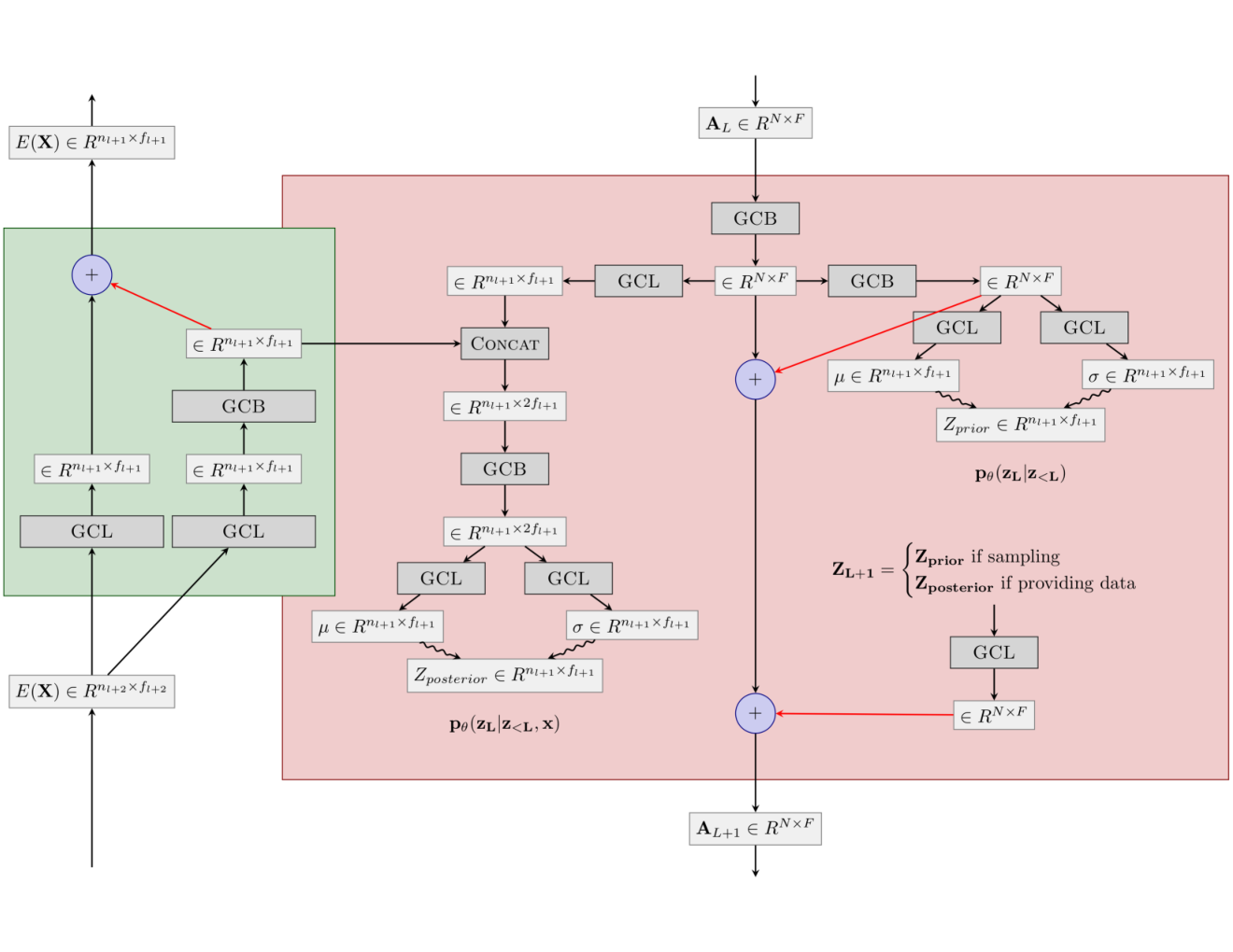
We refer to two main neural network computational blocks as a Graph Convolutional Layer (GCL), which takes as input a graph $A\in\mathbb{R}^{N_{in}\times F_{in}}$ with number of nodes, $N_{in}$ , and number of features, $F_{in}$ , and outputs a new graph with number of nodes, $N_{out}$ , and number of features, $F_{out}$ . $F$ may be considered much like feature channels in a Convolutional Neural Network. For this problem they represent features derived from the frequencies of motion. The second main neural network computational block we refer to as a Graph Convolutional Block (GCB) which takes as input graph $A\in\mathbb{R}^{N_{in}\times F_{in}}$ , and outputs a graph of the same dimensionality. Mathematically, these are defined as

	$\displaystyle\text{GCL}(\mathbf{A})=$	$\displaystyle\sigma\Big(\mathbf{S}\mathbf{A}\mathbf{W}+\mathbf{b}\Big)$		(4)
	$\displaystyle\text{GCB}(\mathbf{A})=$	$\displaystyle\sigma\Big(\mathbf{S_{2}}\sigma\Big(\mathbf{S_{1}}\mathbf{A}\mathbf{W_{1}}+\mathbf{b_{1}}\Big)\mathbf{W_{2}}+\mathbf{b_{2}}\Big)+\alpha\mathbf{A},$		(5)

where in equation 4, $\mathbf{S}\in\mathbb{R}^{N_{out}\times N_{in}}$ , $\mathbf{W}\in\mathbb{R}^{F_{in}\times F_{out}}$ , and $\mathbf{b}\in\mathbb{R}^{N_{out}\times F_{out}}$ are all learnable parameters. Similarly, $\mathbf{S},\mathbf{W},\mathbf{b}\in\mathbb{R}^{N_{in}\times F_{in}}$ , in equation 5, are also learnable parameters. $\alpha$ is a learnable residual weighting that is initialised to $0$ as proposed recently by Bachlechner et al. 2020 as an efficient alternative to batch normalization, Ioffe and Szegedy 2015, to mitigate the effect of covariate shift. $\sigma(\cdot)$ is a Gaussian Error Linear Unit, Hendrycks and Gimpel 2016, (GeLU).

4 Implementation

Network Architecture:

Hierarchically, we present a similar structure to Child Child 2021. In the top down decoders we maintain a principal deterministic route connected to each latent variable such that latent variables may contribute directly to the output without being required to contribute to composite features in dependent variables. This approach increases the speed and stability of training by simplifying the nature of the causal relationships between the latent variables and $\mathbf{x}$ , where possible. All computational blocks are of the form of either equation 4 or equation 5. The encoder-decoder architecture for a single stochastic level is shown in Figure 2.

Training Details:

We use the ELBO, defined by equation 1, to train the network end-to-end using the ADAM optimizer Kingma and Ba 2014, with a learning rate of 0.001 and a batch size of 800. We set $p_{\theta}(\mathbf{x}|\mathbf{z})=\mathcal{N}(\mathbf{\mu(\mathbf{z})},\mathbf{\sigma(\mathbf{z})})$ , where $\mu$ and $\sigma$ are outputs of the final stochastic decoder. On the H3.6M dataset, we appended a one-hot vector to $z_{0}$ to represent each action class.

We use two main techniques for increasing training stability; gradient clipping, enforcing a gradient norm value of $100.0$ , and a similar warm-up procedure for the Kullback-Leibler ( $D_{\text{KL}}$ ) divergence to Sønderby et al. 2016, and Child 2021, increasing its weighting in the loss linearly from $0.001$ to $1.0$ over the first $200$ epochs. We train for a total of 5000 epochs, which requires ca. one week on a NVIDIA GeForce RTX 2070 GPU.

5 Experiments

5.1 Datasets

We are given a motion sequence $\mathbf{X}_{1:N}=\left(\mathbf{x}_{1},\mathbf{x}_{2},\mathbf{x}_{3},\cdots,\mathbf{x}_{N}\right)$ consisting of $N$ consecutive human poses, where $\mathbf{x}_{i}\in\mathbb{R}^{K}$ , with $K$ the number of parameters describing each pose. The temporal components are converted into frequencies using the Discrete Cosine Transformation (DCT) prior to input into the network, and then back to timepoints using the Inverse Discrete Cosine Transformation (IDCT) before being applied to the loss. Further details are supplied in the appendix.

AMASS:

The Archive of Motion Capture as Surface Shapes (AMASS) dataset Mahmood et al. 2019 is the largest open-source human motion dataset, which aggregates a number of mocap datasets, such as CMU, KIT and BMLrub, using a SMPL Loper et al. 2015, Romero et al. 2017 parametrization to obtain a human mesh. SMPL represents a human by a shape vector and joint rotation angles. The shape vector, which encompasses coefficients of different human shape bases, defines the human skeleton. We obtain human poses in 3D by applying forward kinematics to one human skeleton. In AMASS, a human pose is represented by 52 joints, including 22 body joints and 30 hand joints. Since we are interested in skeletal motion, we follow Wei et al. 2020 and discard the hand joints and the 4 static joints, leading to an 18-joint human pose. Further, we also use BMLrub¹¹ 1 Available at https://amass.is.tue.mpg.de/dataset. (522 min. video sequence), as our test set as each sequence consists of one actor performing one type of action. All quantitative results are reported from this dataset. We consider motion sequences of 50 timepoints taking only every second frame. A single datapoint here hence consists of $54$ nodes, and $50$ timepoints. Forming $2700$ dimensional inputs.

Human3.6M (H3.6M):

The H3.6M dataset Ionescu et al. 2011, Ionescu et al. 2013, so called as it contains a selection of 3.6 million 3D human poses and corresponding images, consists of seven actors each performing 15 actions, such as walking, eating, discussion, sitting, and talking on the phone. Martinez et al. 2017, Mao et al. 2019, Li et al. 2020a all follow the same training and evaluation procedure: training their motion prediction model on 6 (5 for train and 1 for cross-validation) of the actors, and use subject 5 as a heldout test set. In this work, we use our model trained on H3.6M to demonstrate most of our qualitative results.

5.2 Baselines

VAE:

A conventional, fully-connected, VAE is trained with $n_{z}=50$ dimensional latent variable and a symmetric encoder-decoder of architecture $2000,1000,500,100,50$ , with batch normalization applied to each layer and trained for $200$ epochs with a learning rate of $0.001$ using the ADAM optimizer. The model has 20.81M parameters.

HM-VAE:

We implement and train the motion prior model proposed by Li et al. 2021. We pool the joints in the upper latent variable to 6 joints, which results in a graph size of 18 at the top latent variable, and 54 on the bottom. In our model, we directly model the scale of the uncertainty in the reconstruction, $\sigma(z)$ , which implicitly learns an appropriate scaling between the two terms in the ELBO (equation 1). However, for HM-VAE we downweight the $D_{\text{KL}}$ divergence by a factor of $0.003$ , as in Li et al. 2018. We otherwise use the same hyperparameters as for our model.

5.3 Experimental setup

We present experiments in support of 3 main arguments for the proficiency of our generative model. First, we degrade the test set data by simulating occlusions wherein, a naive imputation, the mean value of the missing feature over the train set, is substituted for the ground truth. The degree of degradation is controlled by the number of input features occluded. A sufficient level of degradation may be considered as shifting the data out-of-distribution, which we quantify using the model’s posterior. In the appendix we discuss further details and show that this well-informed imputation facilitates better downstream discriminative tasks (see appendix). Second, we examine the effect of stochastic depth, independent of capacity, on performance by training a 16 stochastic-layered model several times with a varying number of its top latent variables turned off ( $z_{L}=\mu_{L}$ , for each level, $L$ , that is turned off, and $KL_{L}$ does not contribute to the loss). Third, we demonstrate that HG-VAE learns an efficient hierarchical ordering that facilitates levels of abstraction, the top of which may represent action classification as well as conditional generation.

6 Results

The average ground truth, test set posterior on H3.6M was $p(z|x)=-9312\pm 500$ . Figure 1, a and b, show two motion sequences (top of each) with the $p(z|x)=-10039$ , and $p(z|x)=-10364$ respectively. The bottom row of a and b show the MAP-imputed values using HG-VAE, with $p(z|x)=-9643$ , and $p(z|x)=-9717$ respectively. A reasonable out-of-distribution (OoD) threshold of the standard deviation of the posterior would both enable the model to detect these OoD examples, and, if the samples are OoD due to occlusion, find the most probable in-distribution representation.

In Figure 4 we consider the MSE between the ground truth and the naive mean imputation; as well as each models’ MAP estimates. We show this as a percentage difference in MSE compared to the MSE of mean imputation. HG-VAE gives a $77\%\pm 1\%$ decrease consistently across all degrees of degradation, which greatly beats baseline methods. The use of MAP estimates from our model give significant improvement in downstream prediction tasks as shown in the appendix.

We investigated how statistical depth, independent of capacity, improved performance. Here a stochastic depth of $1$ is a classical VAE with a very deep encoder, and decoder. Simply, $z_{L}=\mu_{L}$ , for each level $L$ that was turned off, and $KL_{L}$ didn’t contribute to the loss. Table 1 shows that greater stochastic depth achieves higher likelihoods, reconstructions, and KL. Implying that the model benefits greatly from the latent variable dependency structure.

Table 1: HG-VAE Performance as a Function of Stochastic Depth.

Parameters	Stochastic Depth	$\log(\mathbf{X})$	MSE	KL-Divergence
15M	1	$1986$	$2.30$	$274$
15M	2	$3912$	$1.31$	$79$
15M	4	$6511$	$0.59$	$30$
15M	8	$7112$	$0.55$	$32$
15M	16	$7238$	$0.53$	$29$

Figures 3, and 5 show samples from the model trained on H3.6M with different one-hot labels. Figure 5 shows a conditional sample drawn with the label walking from a 4-layer HG-VAE at each level of resolution. 5a is the mean sample drawn from the walking cluster (see appendix), $Z_{i}=\mu_{i}$ , for $i>0$ . We can see that each latent hierarchy adds further expression to the motion sequence. More examples are shown in the appendix.

7 Conclusions

We propose a novel hierarchical graph-convolutional variational autoencoder and demonstrate its ability to learn complex and action-generic latent distributions for human motion that may be used for highly informed imputation and anomaly detection, as well as downstream discriminative tasks. We show that with just 10 gradient ascent steps we obtain a $77\%$ decrease in MSE compared to a mean imputation policy consistently across all degrees of degradation which is greater and more consistent than all baseline models. We demonstrate that stochastic depth matters, independently of model capacity. We further show that the hierarchical latent variables have both enough expression in the lower latent variables ( $z_{i>0}$ ) to model local observables while benefiting from complete abstraction in the top latent variable ( $z_{0}$ ) such that it may be class-conditioned by appending a one-hot vector and produce qualitatively distinct actions. Due to the generality of the architecture, HG-VAE may be a suitable, deeply expressive, generative model for many graph-based domains other than human motion modelling.

8 Limitations and Societal Impact

The method of missing data imputation via gradient ascent on the posterior, though powerful given a good generative model, is expensive. Despite only a small number of parameters—the number of missing features—each step needs almost a complete forward and backward pass through the model. So this may not be an effective method of imputation for online models. However, using a small number of posterior ascent steps is shown to already yield significant improvement, and may be applicable for many online applications. Furthermore, such a model trained on a motion capture dataset such as H3.6M, or AMASS—as is the case here—may be used to very effectively improve motion capture data containing occlusions that is captured in the wild by pose estimation methods. Further work might also include using this model trained on AMASS to synthesise larger datasets. We acknowledge that models capable of learning highly specific motion patterns could be used for nefarious, Orwellian, applications. However, we believe the potential benefit in an ever more automated world, especially in safety in healthcare, outweighs the potential cost.

References

Geertsema et al. [2018] Evelien E Geertsema, Roland D Thijs, Therese Gutter, Ben Vledder, Johan B Arends, Frans S Leijten, Gerhard H Visser, and Stiliyan N Kalitzin. Automated video-based detection of nocturnal convulsive seizures in a residential care setting. Epilepsia, 59:53–60, 2018.
Kakar et al. [2005] Manish Kakar, Håkan Nyström, Lasse Rye Aarup, Trine Jakobi Nøttrup, and Dag Rune Olsen. Respiratory motion prediction by using the adaptive neuro fuzzy inference system (anfis). Physics in Medicine & Biology, 50(19):4721, 2005.
Chang et al. [2012] Chien-Yen Chang, Belinda Lange, Mi Zhang, Sebastian Koenig, Phil Requejo, Noom Somboon, Alexander A Sawchuk, and Albert A Rizzo. Towards pervasive physical rehabilitation using microsoft kinect. In 2012 6th international conference on pervasive computing technologies for healthcare (PervasiveHealth) and workshops, pages 159–162. IEEE, 2012.
Webster and Celik [2014] David Webster and Ozkan Celik. Systematic review of kinect applications in elderly care and stroke rehabilitation. Journal of neuroengineering and rehabilitation, 11(1):108, 2014.
Koppula and Saxena [2013a] Hema Swetha Koppula and Ashutosh Saxena. Anticipating human activities for reactive robotic response. In IROS, page 2071. Tokyo, 2013a.
Koppula and Saxena [2013b] Hema Koppula and Ashutosh Saxena. Learning spatio-temporal structure from rgb-d videos for human activity detection and anticipation. In International conference on machine learning, pages 792–800, 2013b.
Gui et al. [2018a] Liang-Yan Gui, Kevin Zhang, Yu-Xiong Wang, Xiaodan Liang, José MF Moura, and Manuela Veloso. Teaching robots to predict human motion. In 2018 IEEE/RSJ International Conference on Intelligent Robots and Systems (IROS), pages 562–567. IEEE, 2018a.
Paden et al. [2016] Brian Paden, Michal Čáp, Sze Zheng Yong, Dmitry Yershov, and Emilio Frazzoli. A survey of motion planning and control techniques for self-driving urban vehicles. IEEE Transactions on intelligent vehicles, 1(1):33–55, 2016.
Alahi et al. [2016] Alexandre Alahi, Kratarth Goel, Vignesh Ramanathan, Alexandre Robicquet, Li Fei-Fei, and Silvio Savarese. Social lstm: Human trajectory prediction in crowded spaces. In Proceedings of the IEEE conference on computer vision and pattern recognition, pages 961–971, 2016.
Bhattacharyya et al. [2018] Apratim Bhattacharyya, Mario Fritz, and Bernt Schiele. Long-term on-board prediction of people in traffic scenes under uncertainty. In Proceedings of the IEEE Conference on Computer Vision and Pattern Recognition, pages 4194–4202, 2018.
Wang et al. [2019] Yijing Wang, Zhengxuan Liu, Zhiqiang Zuo, Zheng Li, Li Wang, and Xiaoyuan Luo. Trajectory planning and safety assessment of autonomous vehicles based on motion prediction and model predictive control. IEEE Transactions on Vehicular Technology, 68(9):8546–8556, 2019.
Švec et al. [2014] Petr Švec, Atul Thakur, Eric Raboin, Brual C Shah, and Satyandra K Gupta. Target following with motion prediction for unmanned surface vehicle operating in cluttered environments. Autonomous Robots, 36(4):383–405, 2014.
Shirai et al. [2007] Akihiko Shirai, Erik Geslin, and Simon Richir. Wiimedia: motion analysis methods and applications using a consumer video game controller. In Proceedings of the 2007 ACM SIGGRAPH symposium on Video games, pages 133–140, 2007.
Rofougaran et al. [2018] Ahmadreza Reza Rofougaran, Maryam Rofougaran, Nambirajan Seshadri, Brima B Ibrahim, John Walley, and Jeyhan Karaoguz. Game console and gaming object with motion prediction modeling and methods for use therewith, April 17 2018. US Patent 9,943,760.
Lau and Chan [2008] Rynson WH Lau and Addison Chan. Motion prediction for online gaming. In International Workshop on Motion in Games, pages 104–114. Springer, 2008.
Bourached and Cann [2019] Anthony Bourached and George Cann. Raiders of the lost art. arXiv preprint arXiv:1909.05677, 2019.
Bourached et al. [2021] Anthony Bourached, George H Cann, Ryan-Rhys Griffths, and David G Stork. Recovery of underdrawings and ghost-paintings via style transfer by deep convolutional neural networks: A digital tool for art scholars. Electronic Imaging, 2021(14):42–1, 2021.
Cann et al. [2021] George H Cann, Anthony Bourached, Ryan-Rhys Griffths, and David G Stork. Resolution enhancement in the recovery of underdrawings via style transfer by generative adversarial deep neural networks. Electronic Imaging, 2021(14):17–1, 2021.
Stork et al. [2021] David G Stork, Anthony Bourached, George H Cann, and Ryan-Rhys Griffths. Computational identification of significant actors in paintings through symbols and attributes. Electronic Imaging, 2021(14):15–1, 2021.
Kell et al. [2022] Gregory Kell, Ryan-Rhys Griffiths, Anthony Bourached, and David G Stork. Extracting associations and meanings of objects depicted in artworks through bi-modal deep networks. arXiv preprint arXiv:2203.07026, 2022.
Kim and Paik [2010] Daehee Kim and J Paik. Gait recognition using active shape model and motion prediction. IET Computer Vision, 4(1):25–36, 2010.
Ma et al. [2018] Zhuo Ma, Xinglong Wang, Ruijie Ma, Zhuzhu Wang, and Jianfeng Ma. Integrating gaze tracking and head-motion prediction for mobile device authentication: A proof of concept. Sensors, 18(9):2894, 2018.
Grant et al. [2019] James Grant, Alexis Boukouvalas, Ryan-Rhys Griffiths, David Leslie, Sattar Vakili, and Enrique Munoz De Cote. Adaptive sensor placement for continuous spaces. In International Conference on Machine Learning, pages 2385–2393. PMLR, 2019.
Bachlechner et al. [2020] Thomas Bachlechner, Bodhisattwa Prasad Majumder, Huanru Henry Mao, Garrison W Cottrell, and Julian McAuley. Rezero is all you need: Fast convergence at large depth. arXiv preprint arXiv:2003.04887, 2020.
Fragkiadaki et al. [2015] Katerina Fragkiadaki, Sergey Levine, Panna Felsen, and Jitendra Malik. Recurrent network models for human dynamics. In Proceedings of the IEEE International Conference on Computer Vision, pages 4346–4354, 2015.
Jain et al. [2016] Ashesh Jain, Amir R Zamir, Silvio Savarese, and Ashutosh Saxena. Structural-rnn: Deep learning on spatio-temporal graphs. In Proceedings of the ieee conference on computer vision and pattern recognition, pages 5308–5317, 2016.
Martinez et al. [2017] Julieta Martinez, Michael J Black, and Javier Romero. On human motion prediction using recurrent neural networks. In Proceedings of the IEEE Conference on Computer Vision and Pattern Recognition, pages 2891–2900, 2017.
Pavllo et al. [2018] Dario Pavllo, David Grangier, and Michael Auli. Quaternet: A quaternion-based recurrent model for human motion. arXiv preprint arXiv:1805.06485, 2018.
Gui et al. [2018b] Liang-Yan Gui, Yu-Xiong Wang, Xiaodan Liang, and José MF Moura. Adversarial geometry-aware human motion prediction. In Proceedings of the European Conference on Computer Vision (ECCV), pages 786–803, 2018b.
Guo and Choi [2019] Xiao Guo and Jongmoo Choi. Human motion prediction via learning local structure representations and temporal dependencies. In Proceedings of the AAAI Conference on Artificial Intelligence, volume 33, pages 2580–2587, 2019.
Gopalakrishnan et al. [2019] Anand Gopalakrishnan, Ankur Mali, Dan Kifer, Lee Giles, and Alexander G Ororbia. A neural temporal model for human motion prediction. In Proceedings of the IEEE Conference on Computer Vision and Pattern Recognition, pages 12116–12125, 2019.
Li et al. [2020a] Maosen Li, Siheng Chen, Yangheng Zhao, Ya Zhang, Yanfeng Wang, and Qi Tian. Dynamic multiscale graph neural networks for 3d skeleton based human motion prediction. In Proceedings of the IEEE/CVF Conference on Computer Vision and Pattern Recognition, pages 214–223, 2020a.
Butepage et al. [2017] Judith Butepage, Michael J Black, Danica Kragic, and Hedvig Kjellstrom. Deep representation learning for human motion prediction and classification. In Proceedings of the IEEE conference on computer vision and pattern recognition, pages 6158–6166, 2017.
Li et al. [2018] Chen Li, Zhen Zhang, Wee Sun Lee, and Gim Hee Lee. Convolutional sequence to sequence model for human dynamics. In Proceedings of the IEEE Conference on Computer Vision and Pattern Recognition, pages 5226–5234, 2018.
Mao et al. [2019] Wei Mao, Miaomiao Liu, Mathieu Salzmann, and Hongdong Li. Learning trajectory dependencies for human motion prediction. In Proceedings of the IEEE International Conference on Computer Vision, pages 9489–9497, 2019.
Wei et al. [2020] Mao Wei, Liu Miaomiao, and Salzemann Mathieu. History repeats itself: Human motion prediction via motion attention. In ECCV, 2020.
Wang et al. [2021] Jingbo Wang, Sijie Yan, Bo Dai, and Dahua Lin. Scene-aware generative network for human motion synthesis. In Proceedings of the IEEE/CVF Conference on Computer Vision and Pattern Recognition, pages 12206–12215, 2021.
Yan et al. [2019] Sijie Yan, Zhizhong Li, Yuanjun Xiong, Huahan Yan, and Dahua Lin. Convolutional sequence generation for skeleton-based action synthesis. In Proceedings of the IEEE/CVF International Conference on Computer Vision (ICCV), October 2019.
Barsoum et al. [2018] Emad Barsoum, John Kender, and Zicheng Liu. Hp-gan: Probabilistic 3d human motion prediction via gan. In Proceedings of the IEEE conference on computer vision and pattern recognition workshops, pages 1418–1427, 2018.
Cai et al. [2018] Haoye Cai, Chunyan Bai, Yu-Wing Tai, and Chi-Keung Tang. Deep video generation, prediction and completion of human action sequences. In Proceedings of the European Conference on Computer Vision (ECCV), pages 366–382, 2018.
Ling et al. [2020] Hung Yu Ling, Fabio Zinno, George Cheng, and Michiel Van De Panne. Character controllers using motion vaes. ACM Transactions on Graphics (TOG), 39(4):40–1, 2020.
Li et al. [2021] Jiaman Li, Ruben Villegas, Duygu Ceylan, Jimei Yang, Zhengfei Kuang, Hao Li, and Yajie Zhao. Task-generic hierarchical human motion prior using vaes. arXiv preprint arXiv:2106.04004, 2021.
Kipf and Welling [2016] Thomas N Kipf and Max Welling. Semi-supervised classification with graph convolutional networks. arXiv preprint arXiv:1609.02907, 2016.
Niepert et al. [2016] Mathias Niepert, Mohamed Ahmed, and Konstantin Kutzkov. Learning convolutional neural networks for graphs. In International conference on machine learning, pages 2014–2023. PMLR, 2016.
Yan et al. [2018] Sijie Yan, Yuanjun Xiong, and Dahua Lin. Spatial temporal graph convolutional networks for skeleton-based action recognition. In Thirty-second AAAI conference on artificial intelligence, 2018.
Bourached et al. [2020] Anthony Bourached, Ryan-Rhys Griffiths, Robert Gray, Ashwani Jha, and Parashkev Nachev. Generative model-enhanced human motion prediction. arXiv preprint arXiv:2010.11699, 2020.
Kingma and Welling [2013] Diederik P Kingma and Max Welling. Auto-encoding variational bayes. arXiv preprint arXiv:1312.6114, 2013.
Sønderby et al. [2016] Casper Kaae Sønderby, Tapani Raiko, Lars Maaløe, Søren Kaae Sønderby, and Ole Winther. Ladder variational autoencoders. Advances in neural information processing systems, 29:3738–3746, 2016.
Child [2021] Rewon Child. Very deep vaes generalize autoregressive models and can outperform them on images, 2021.
Lawrence et al. [1997] Steve Lawrence, C Lee Giles, Ah Chung Tsoi, and Andrew D Back. Face recognition: A convolutional neural-network approach. IEEE transactions on neural networks, 8(1):98–113, 1997.
Li et al. [2020b] Maosen Li, Siheng Chen, Yangheng Zhao, Ya Zhang, Yanfeng Wang, and Qi Tian. Dynamic multiscale graph neural networks for 3d skeleton based human motion prediction. In Proceedings of the IEEE/CVF Conference on Computer Vision and Pattern Recognition, pages 214–223, 2020b.
Ioffe and Szegedy [2015] Sergey Ioffe and Christian Szegedy. Batch normalization: Accelerating deep network training by reducing internal covariate shift. In International conference on machine learning, pages 448–456. PMLR, 2015.
Hendrycks and Gimpel [2016] Dan Hendrycks and Kevin Gimpel. Bridging nonlinearities and stochastic regularizers with gaussian error linear units. 2016.
Kingma and Ba [2014] Diederik P Kingma and Jimmy Ba. Adam: A method for stochastic optimization. arXiv preprint arXiv:1412.6980, 2014.
Mahmood et al. [2019] Naureen Mahmood, Nima Ghorbani, Nikolaus F Troje, Gerard Pons-Moll, and Michael J Black. Amass: Archive of motion capture as surface shapes. In Proceedings of the IEEE/CVF International Conference on Computer Vision, pages 5442–5451, 2019.
Loper et al. [2015] Matthew Loper, Naureen Mahmood, Javier Romero, Gerard Pons-Moll, and Michael J Black. Smpl: A skinned multi-person linear model. ACM transactions on graphics (TOG), 34(6):1–16, 2015.
Romero et al. [2017] Javier Romero, Dimitrios Tzionas, and Michael J Black. Embodied hands: Modeling and capturing hands and bodies together. ACM Transactions on Graphics (ToG), 36(6):1–17, 2017.
Ionescu et al. [2011] Catalin Ionescu, Fuxin Li, and Cristian Sminchisescu. Latent structured models for human pose estimation. In 2011 International Conference on Computer Vision, pages 2220–2227. IEEE, 2011.
Ionescu et al. [2013] Catalin Ionescu, Dragos Papava, Vlad Olaru, and Cristian Sminchisescu. Human3.6m: Large scale datasets and predictive methods for 3d human sensing in natural environments. IEEE transactions on pattern analysis and machine intelligence, 36(7):1325–1339, 2013.
McInnes et al. [2018] Leland McInnes, John Healy, and James Melville. Umap: Uniform manifold approximation and projection for dimension reduction. arXiv preprint arXiv:1802.03426, 2018.

Appendix

The appendix consists of 3 parts. We provide a brief summary of each section below.

Appendix A: we provide an elaboration of the formulation of the data and the equations used to transform the temporal component of the data before input to the model, as well as after output.

Appendix B: we provide further results and explanation of the imputation experiments available in the main text.

Appendix C: we provide experiments that demonstrates the quantitative improvement of predictive tasks achieved by imputation via gradient ascent on HGVAE’s posterior.

We further provides gifs of samples from the model.

Appendix A Problem formulation

A.1 DCT-based Temporal Encoding

Mao et al. 2019 proposed transforming the temporal component of human motion to frequencies using Discrete Cosine Transformations (DCT). In this way each resulting coefficient encodes information of the entire sequence at a particular temporal frequency. Furthermore, the option to remove high or low frequencies is provided. Given a joint, $k$ , the position of $k$ over $N$ time steps is given by the trajectory vector: $\mathbf{x}_{k}=[x_{k,1},\ldots,x_{k,N}]$ where we convert to a DCT vector of the form: $\mathbf{C}_{k}=[C_{k,1},\ldots,C_{k,N}]$ where $C_{k,l}$ represents the lth DCT coefficient. For $\mathbf{\delta}_{l1}\in\mathbb{R}^{N}=[1,0,\cdots,0]$ , these coefficients may be computed as

\displaystyle C_{k,l}=\sqrt{\frac{2}{N}}\sum_{n=1}^{N}x_{k,n}\frac{1}{\sqrt{1+\delta_{l1}}}\cos\left(\frac{\pi}{2N}(2n-1)(l-1)\right).

(6)

If no frequencies are cropped, the DCT is invertible via the Inverse Discrete Cosine Transform (IDCT):

\displaystyle x_{k,l}=\sqrt{\frac{2}{N}}\sum_{l=1}^{N}C_{k,l}\frac{1}{\sqrt{1+\delta_{l1}}}\cos\left(\frac{\pi}{2N}(2n-1)(l-1)\right).

(7)

We find this lossless transformation effectively creates a feature space that is much more conducive for optimisation. The objective is still to learn $p(x)$ .

Appendix B Imputation

Figure 6 shows the initial posterior of the degraded input as well as the final after 10 steps, a $p(z|x)_{\text{MAP}}$ estimate, of gradient ascent on the model’s posterior. For the HG-VAE (6b) the average posterior already lies outside the standard deviation of the ground truth for just 0.5% of features occluded, demonstrating acute out-of-distribution detection. In contrast, the VAE’s average posterior only falls outside a standard deviation of the ground truth for approximately 50% occlusion. A fully expressive model should not, on average, give a higher MAP estimate than the posterior on the ground truth. The evidence of this in Figure 6a indicates that the model lacks the capacity to delineate latent features representative of the full expressivity of $x$ , and hence gives a higher probability to a closer to average expression than the ground truth.

We see no evidence of this lack of expressivity in Figure 6b. In fact, the MAP estimate strictly upper-bounds the mean imputation, $p(z|x)_{\text{init}}$ , and is strictly upper-bounded by the ground truth ( $p(z|x)_{\text{GT}}$ ).

Imputation of missing data:

Given occluded inputs, and a sufficiently expressive $p(z|x)$ , it is possible to gradient ascent the missing inputs on the model’s posterior. If the model’s maximum a posteriori (MAP), given the partially observed datapoint, is close to the ground truth, $x$ , this will result in a statistically well-informed imputation. For these experiments we use the Adam optimiser on the negative log posterior ( $-\sum_{i}\log\big(p(z_{i}|x)\big)$ ) and select a learning rate that is sufficiently low for stable descent. This was 100.0 for the VAE and 1.0 for HG-VAE, and HM-VAE (this difference is proportional to the difference in magnitude of the average log posterior for the respective models). We gradient ascended on $800$ datapoints at once, for a maximum of $10$ steps selecting the step of highest model posterior for each datapoint.

Figure 7 shows the results from Figure 6b as a percentage change in the negative log posterior. We can see that the change on a logarithmic scale is consistent over all degrees of degradation indicating the sensitivity of the model to subtle changes in the observables.

Appendix C Improved downstream tasks

We demonstrate the MAP-estimates for the missing values given by our model facilitate better downstream discriminative tasks by considering the degradation in performance of three deterministic deep network motion prediction models, convSeq2Seq Li et al. 2018, LTD Mao et al. 2019, and HisRepItself Wei et al. 2020 under feature occlusion. We train each model on 50 timepoints, to predict the next 25. At test time we randomly occlude the input features and report the error on the predicted future trajectory. We report the Mean Per Joint Position Error (MPJPE) Ionescu et al. 2013 given by

\displaystyle\ell_{m}=\frac{1}{J(N+T)}\sum_{n=1}^{N+T}\sum_{j=1}^{J}\left\|\hat{\mathbf{p}}_{j,n}-\mathbf{p}_{j,n}\right\|^{2}

(8)

where $\hat{\mathbf{p}}_{j,n}\in\mathbb{R}^{3}$ denotes the predicted jth joint position in frame $n$ . And $\mathbf{p}_{j,n}$ is the corresponding ground truth, while J is the number of joints in the skeleton. We compare the raw performance given mean imputation against the MAP estimates obtained by performing 100 steps of gradient ascent on HG-VAE’s posterior.

The use of MAP estimates from our model give significant improvement in downstream prediction tasks as shown in figure 8.

We use Uniform Manifold Approximation and Prediction (UMAP) McInnes et al. 2018, to project the top latent variables of 1000 random samples, conditioned on one-hot encodings, onto a 2-dimensional plane. We show two contrasting actions in figure 9, walking, and sitting. We can see that a very clear separation between the two different actions showing that there is a strong level of abstraction in the top latent variable.


a) Posterior, $p(z\|x)$ (VAE baseline)	b) Posterior, $p(z\|x)$ (HG-VAE)