Optimization-free Ground Contact Force Constraint Satisfaction in Quadrupedal Locomotion
Abstract
We are seeking control design paradigms for legged systems that allow bypassing costly algorithms that depend on heavy on-board computers widely used in these systems and yet being able to match what they can do by using less expensive optimization-free frameworks. In this work, we present our preliminary results in modeling and control design of a quadrupedal robot called Husky Carbon, which under development at Northeastern University (NU) in Boston. In our approach, we utilized a supervisory controller and an Explicit Reference Governor (ERG) to enforce ground reaction force constraints. These constraints are usually enforced using costly optimizations. However, in this work, the ERG manipulates the state references applied to the supervisory controller to enforce the ground contact constraints through an updated law based on Lyapunov stability arguments. As a result, the approach is much faster to compute than the widely used optimization-based methods.
I Introduction
In this work, we will report our preliminary results in the modeling, control design, and development of a legged robot called NU’s Husky Carbon (shown in Fig. 1). Our objective is to integrate legged and aerial mobility into a single platform.
Robotic biomimicry of animals’ multi-modal locomotion can be a significant ordeal. The prohibitive design restrictions such as tight power budget, limited payload, complex multi-modal actuation and perception, an excessive number of active and passive joints involved in each mode, sophisticated control, and environment-specific models, just to name a few, have alienated these concepts. It is worth noting that as how multi-modality has secured birds’ (and other species) survival in complex environments, similar manifestations in mobile robots can be rewarding and important.

Payload is a key factor for aerial systems. We are seeking control design paradigms that allow bypassing costly algorithms that depend on heavy on-board computers widely used in legged systems and yet being able to match what they can do using less expensive optimization-free frameworks. In this work, we will present our optimization-free approach based on path planning in the state space of the robot. Our constraints are bounded unilateral ground contact forces which are important to avoid the violation of gait feasibility conditions. The resulting algorithms can run faster and can be hosted by lightweight processors.
From a feedback design standpoint, the challenge of simultaneously providing asymptotic stability and gait feasibility constraints satisfaction in legged systems (bipedal and multi-pedal) has been extensively addressed [1, 2, 3]. For instance, the works by [4] have provided rigorous model-based approaches to assign attributes such as the efficiency of locomotion in off-line fashions.
Other attempts entail optimization-based, nonlinear approaches to secure safety and performance of legged locomotion [5, 6, 7, 8, 9]. In general, in these paradigms, an optimization-based controller adjusts the gait parameters throughout the whole gait cycle such that not only the robot’s posture is adjusted to accommodate the unplanned posture adjustments but also the joints position, velocity, and acceleration are modified to avoid slipping into infeasible scenarios, e.g., the violation of contact forces. What makes these methods cumbersome is that they are widely defined based on whole-body control at every time-step which can lead to computationally expensive optimization problems.
Many of today’s real-time approaches have achieved better efficiencies through reduced-order models and decomposition methods [10], however, they still depend on optimization solvers [11, 12, 13, 14, 15, 16, 17, 18, 19, 20]. While many optimization-based methods do not present promising horizons in experimental legged robotics, other Gauss-Newton Hessian approximation such as Sequential Linear Quadratic (SLQ) [21], iLQR and iLQG [22] have been more effective. That said, they also present formidable challenges for smaller processors.
Other popular paradigms such as Approximate Dynamic Programming (ADP) [23], Reinforcement Learning (RL) [24], decoupled approaches to design control for nonlinear stochastic systems [25] can potentially remedy the challenges associated with costs of computation. However, these approaches are far from providing any practical solutions to the problem at hand and they are shown to be only effective on simpler practical robots [26, 27, 28, 29, 30, 31, 32, 33] and demonstrations in more complex problems such as those offered by legged robots are missing.
In this work, we will resolve gait parameters for our quadrupedal platform off-line and re-plan them in real-time during the gait cycle. We assume well-tuned supervisory controllers found in [34, 35, 36] and will focus on fine-tuning the joints’ desired trajectories to satisfy unilateral contact force constraints. To do this, we will devise intermediary filters based on Explicit Reference Governors (ERG) [37, 38, 39, 40, 41, 42]. ERGs relied on provable Lyapunov stability properties can perform the motion planning problem in the state space in a much faster way than widely used optimization-based methods.
II Overview of Northeastern University’s Husky Carbon Morpho-functional Platform
Husky Carbon [43], shown in Fig. 1, when standing as a quadrupedal robot, is 2.5 ft (0.8 m) tall, is 12 in (0.3 m) wide. The robot was fabricated from reinforced thermoplastic materials through additive manufacturing with a total weight of 9.5 lb (4.3 kg). It hosts on-board power electronics and it operates using an external power supply. The current prototype lacks exteroceptive sensors such as camera and LiDAR. The robot is constructed of two pairs of identical legs in the form of parallelogram mechanisms. Each with three degrees-of-freedom (DOFs), the legs are fixated to Husky’s torso by a one-DOF revolute joint with a large range of motion. As a result, the legs can be located sideways. This configuration allows facing the knee actuators upwards for propulsion purposes. A clutch mechanism will disengage the knee actuator from the lower limb before the actuator runs a propeller.
III System dynamic modeling and controller
Husky can be modeled using the simple reduced-order model where the leg is assumed to be massless and all masses are incorporated into the body. Then the system has 6 dynamical DOFs representing the body’s linear position and orientation. Each leg is modeled using two hip angles (frontal and sagittal) and a prismatic joint to describe the leg end position. This results in a very simplified model which we will use in a numerical simulation.
III-A Husky Reduced Order Model (HROM)
The Husky Reduced Order Model (HROM) can be derived using Euler-Lagrangian dynamics formulation where the full conformation of Husky as shown in Fig. 1 are simplified by assuming massless legs and modeling them as variable-length linkages from the center of mass to the foot end positions. These virtual legs can be defined using two rotations and length variables, and the ground reaction forces (GRF) are applied at the foot end positions which will perturb the system.
Let the superscript represent a vector defined in the body frame (e.g., ), and the rotation matrix represents the rotation of a vector from the body frame to the inertial frame (e.g., ). The foot end positions can be derived using the following kinematics equations:
| (1) | ||||
where is the body position, is the position of foot where is the set of legs, and are the hip frontal and sagittal angles respectively, and is the prismatic joint length.
Let be the body angular velocity in the body frame and be the gravitational acceleration vector. The legs of HROM are massless, so we can ignore all leg states and directly calculate the kinetic energy and potential energy . Then the Lagrangian of the system can be calculated as and the dynamic equation of motion can be derived using the Euler-Lagrangian Method. The body orientation is defined using the Hamiltonian’s principles and the modified Lagrangian for rotation in SO(3) to avoid using Euler rotations which can become singular during the simulation. Then the equation of motion can be derived as follows:
| (2) |
where and are the generalized vectors, is the skew operator, and . The dynamic system acceleration can then be solved from into the following standard form:
| (3) |
where is the mass/inertia matrix, contains the coriolis and gravitational vectors, represent the generalized force due to the GRF () acting on the foot , and where . , , and are also a function of the leg joint variables (, , and ), which is driven by setting their accelerations to track a desired joint states. The joint states and the inputs are defined as follows
| (4) |
where , , and contain the joint variables of all legs (hip frontal, hip sagittal, and leg length respectively), and forms the control input to the system in the form of the leg joint state accelerations. Combining both the dynamic and massless leg states form the full system states:
| (5) |
where the contains the elements of the rotation matrix . The equation of motion can then simply defined as which will be implemented in a numerical simulation.
The GRF is modeled using a compliant ground model and Stribeck friction model, defined as follows:
| (6) | ||||
where and are the and positions of foot respectively, and are the spring and damping coefficients of the compliant surface model respectively, and are the ground friction forces respectively, , , and are the Coulomb, static, and viscous friction coefficients respectively, and is the Stribeck velocity. We omit the derivations of as it follows similar derivations to .
III-B Controller and Explicit Reference Governor (ERG)

The ERG framework is used to enforce the ground force constraint during the implementation of the walking gait. The ERG is utilized by defining a cost or constraint equation as a function of the controller reference. However, calculating the GRF is very complex and difficult even in HROM, so a further simplified model is used to estimate the GRF and to derive the constraint equations.
The ROM is modeled as a triangular inverted pendulum (TIP), shown in Fig. 2, which is an extension of the more standard variable length inverted pendulum model. The two contact points at the feet allow us to estimate the distribution of GRF between the two legs so we can evaluate the friction constraint on each leg individually. The kinematic constraints of the TIP model can be defined as follows:
| (7) |
where and are the front and rear foot position respectively and represent the leg position from the body CoM to either foot. Assuming no slippage at the foot end points (), the body can be controlled using the leg length acceleration . In this case, the body acceleration is the control input to this simplified model which will be mapped back into the joint space accelerations () for HROM. Consider the following PD controller to track a desired body states () and velocity:
| (8) |
where and are the PD gains for this controller. Define the vectors and which turns (8) into the concise form of where .
The ground forces can be derived from the body acceleration, as this point mass dynamics can be modeled as follows:
| (9) |
where and are the GRF of the front and rear foot respectively. Since we can only solve for the sum of the ground forces from (9), we need to make some assumptions to solve for and . This model restricts moment about the axis perpendicular to the support polygon and by assuming the lateral ground forces are distributed evenly, we can form the following constraint equations:
| (10) |
where is the unit vector perpendicular to the support polygon along the ground plane, and and are the distance along the support polygon as illustrated in Fig. 2. Combining (9) and (10) yields the general form equation where the GRF can be solved given that is invertible. The GRF can be defined as a function of the body position reference by plugging in (8) into (9) which will be used to derive the constraint equations for the ERG.
IV Explicit Reference Governor
Explicit reference governor (ERG) works as an add-on scheme on a pre-stabilized closed-loop system [44]. The ERG manipulates the applied reference to the controller to enforce the desired constraints while being as close as possible to the desired reference trajectory.
IV-A Constraint Equation Formulations
Some constraint equations are defined to enforce the no-slip condition on both stance feet of the robot. Let the constrain equation be defined as follows:
| (11) |
where the relationship between the constraint and is linear. The GRF for both feet can be solved using (8) to (10), as follows:
| (12) |
which is linear in . The following GRF constraints are used to prevent slipping:
| (13) |
Then the constraint equations can be formulated as follows:
| (14) |
for leg . The and in (11) can be calculated numerically using (12) and (14) which will be used to formulate the ERG applied reference update law.
IV-B ERG Formulations

The ERG framework is utilized to enforce the friction pyramid constraint in (14) which is formulated into the form shown in (11). The ERG algorithm manipulates the applied reference into the controller in (8) such that (11) is satisfied. This method is very useful as it avoids using optimization or nonlinear MPC frameworks to enforce constraints on the harder-to-model GRFs.
Let be the applied reference which will be used in the controller instead of , and be the constraint equation value using . The ERG manipulates the applied reference () to avoid violating the constraint equation while also be as close as possible to the desired reference (), as illustrated in Fig. 3. Consider the Lyapunov equation . is updated through the update law:
| (15) |
where drives directly to , while and drives along the surface and into the boundary , respectively. The objective of this ERG algorithm is to drive to the state which is the minimum energy solution that satisfies the constraint . The overall structure of this algorithm can be seen in Algorithm 1.
Let be the rowspace of the violated constraints of (rows of the where the constraint is violated). Define where is the size of the nullspace. Additionally, let be the ’th row of . Then the following update law is used for , , and :
| (16) |
where are scalars defined as follows:
| (17) | ||||
where is a positive scalar which determines the rate of convergence.
Assuming and using the update law defined from (16) and (17), we will have , with . We have the gradient if and , while when or when . In case both applied reference and target constraints equation are violated, we have which drives the towards the constraint boundary. This allows the to converge to which is the minimum energy solution that satisfies as illustrated in Fig. 3.
V Numerical Simulation


The simulation was implemented on HROM based on a predefined quasi-static trotting gait in MATLAB. The stance-swing pair switching was done by using a timing-based state machine, where the gait period is defined as 0.25 s and a total of 20 walking steps was simulated. The input of the ERG and the stance foot controller in (8) is defined as the inertial frame foot end acceleration relative to the current body position. To implement this controller, we simply integrated this acceleration to the desired position and velocity about the body frame, and track these positions using a PID controller. The swing foot trajectory follows a simple bezier curve trajectory with an end position located at a fixed position relative to the body (0.08 m ahead of hip position in the x-axis). The bezier curve trajectory initial position is set as the previous stance foot final position and a target swing height of 0.2 m with zero initial and final velocity. Since we have no row, pitch, or yaw compensation, we rotate the reference by at every time step so that the robot acts like walking on a flat surface without angular deviation.
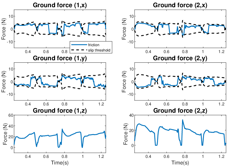
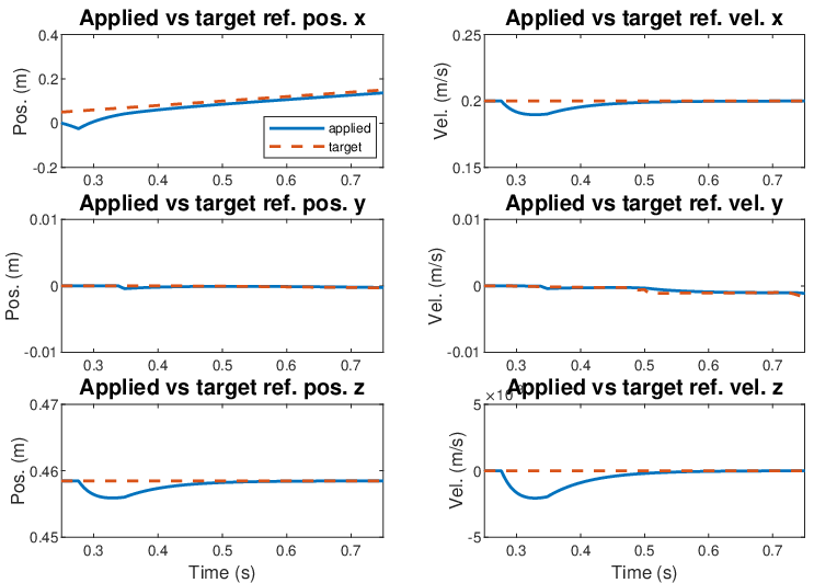
The simulation results of the robot walking on slippery surface () at the target forward speed of 0.2 m/s is shown in Fig. 4 to 7. The resulting gait is stable, with a potential slipping happening at the beginning of the gait which is regulated by the ERG as shown in Fig. 5 and 7. The ERG has successfully manipulated the controller reference states to avoid constraint violation which resulted in a stable trotting gait even on a slippery surface. Figure 5 shows the actual GRF applied to this robot during this simulation and the friction is kept within the constraint boundary defined in (13).
This simulation was performed in Matlab using a computer with AMD Ryzen six-core 3.40 GHz processor and 16 GB of RAM. Each simulation time step which includes the ERG computation and ODE integration with 4th order Runge-Kutta algorithm was computed at a rate of approximately 2 kHz. Most embedded systems are programmed in C or C++ which are significantly faster than Matlab. This shows that our ERG algorithm can be utilized in real-time computations using the robot’s on-board computer.
VI Conclusions and future work
We explored the performance of the ERG algorithm on a quadruped where the no-slip constraints have been enforced successfully. The use of ERG allows the robot to walk stably on a slippery surface () where the controller states are manipulated to satisfy the GRF constraints we specified. This algorithm can be computed quickly, which means that it can serve as an alternative to the more computationally expensive algorithms for enforcing constraints, such as optimization and whole-body control.
The controller considered in this work is only defined for the stance foot where the GRF is applied. Future work should include the usage of the swing foot placement algorithm to regulate the robot heading and the tracking of more complex trajectories. Additionally, other constraints can also be considered for the ERG, such as input and state saturation constraints which are practical for the implementation in the actual robot.
References
- [1] T. Apgar, P. Clary, K. Green, A. Fern, and J. Hurst, “Fast Online Trajectory Optimization for the Bipedal Robot Cassie,” in Robotics: Science and Systems XIV, 2018.
- [2] G. Bledt, “Regularized predictive control framework for robust dynamic legged locomotion,” Ph.D. dissertation, Massachusetts Institute of Technology, 2020.
- [3] M. Hutter et al., “ANYmal - a highly mobile and dynamic quadrupedal robot,” in 2016 IEEE/RSJ International Conference on Intelligent Robots and Systems (IROS), 2016, pp. 38–44.
- [4] E. Westervelt and J. Grizzle, Feedback Control of Dynamic Bipedal Robot Locomotion, ser. Control and Automation Series. CRC PressINC, 2007. [Online]. Available: https://books.google.com/books?id=xaMeAQAAIAAJ
- [5] Q. Nguyen and K. Sreenath, “Optimal robust control for bipedal robots through control lyapunov function based quadratic programs.” in Robotics: Science and Systems, 2015.
- [6] K. Galloway, K. Sreenath, A. D. Ames, and J. W. Grizzle, “Torque saturation in bipedal robotic walking through control lyapunov function-based quadratic programs,” IEEE Access, vol. 3, pp. 323–332, 03 2015.
- [7] A. D. Ames, K. Galloway, K. Sreenath, and J. W. Grizzle, “Rapidly Exponentially Stabilizing Control Lyapunov Functions and Hybrid Zero Dynamics,” IEEE Transactions on Automatic Control, vol. 59, no. 4, pp. 876–891, Apr. 2014.
- [8] A. Hereid, E. A. Cousineau, C. M. Hubicki, and A. D. Ames, “3d dynamic walking with underactuated humanoid robots: A direct collocation framework for optimizing hybrid zero dynamics,” in 2016 IEEE International Conference on Robotics and Automation (ICRA). IEEE, 2016, pp. 1447–1454.
- [9] L. Sentis and O. Khatib, “A whole-body control framework for humanoids operating in human environments,” in Proceedings 2006 IEEE International Conference on Robotics and Automation, 2006. ICRA 2006. IEEE, 2006, pp. 2641–2648.
- [10] T. Buschmann, S. Lohmeier, M. Bachmayer, H. Ulbrich, and F. Pfeiffer, “A collocation method for real-time walking pattern generation,” in 2007 7th IEEE-RAS International Conference on Humanoid Robots, 2007, pp. 1–6.
- [11] T. Koolen et al., “Design of a Momentum-Based Control Framework and Application to the Humanoid Robot Atlas,” International Journal of Humanoid Robotics, vol. 13, no. 01, 2016.
- [12] S. Fahmi, C. Mastalli, M. Focchi, and C. Semini, “Passive Whole-Body Control for Quadruped Robots: Experimental Validation Over Challenging Terrain,” IEEE Robotics and Automation Letters, vol. 4, no. 3, pp. 2553–2560, 2019.
- [13] C. Dario Bellicoso, C. Gehring, J. Hwangbo, P. Fankhauser, and M. Hutter, “Perception-less terrain adaptation through whole body control and hierarchical optimization,” in 2016 IEEE-RAS 16th International Conference on Humanoid Robots (Humanoids), Nov. 2016, pp. 558–564, iSSN: 2164-0580.
- [14] T. Bretl and S. Lall, “Testing Static Equilibrium for Legged Robots,” IEEE Transactions on Robotics, vol. 24, no. 4, pp. 794–807, Aug. 2008.
- [15] D. Pardo, L. Möller, M. Neunert, A. W. Winkler, and J. Buchli, “Evaluating Direct Transcription and Nonlinear Optimization Methods for Robot Motion Planning,” IEEE Robotics and Automation Letters, vol. 1, no. 2, pp. 946–953, Jul. 2016.
- [16] C. Mastalli, M. Focchi, I. Havoutis, A. Radulescu, S. Calinon, J. Buchli, D. G. Caldwell, and C. Semini, “Trajectory and foothold optimization using low-dimensional models for rough terrain locomotion,” in 2017 IEEE International Conference on Robotics and Automation (ICRA), May 2017, pp. 1096–1103.
- [17] C. Mastalli, I. Havoutis, A. W. Winkler, D. G. Caldwell, and C. Semini, “On-line and on-board planning and perception for quadrupedal locomotion,” in 2015 IEEE International Conference on Technologies for Practical Robot Applications (TePRA), May 2015, pp. 1–7.
- [18] A. W. Winkler, C. D. Bellicoso, M. Hutter, and J. Buchli, “Gait and Trajectory Optimization for Legged Systems Through Phase-Based End-Effector Parameterization,” IEEE Robotics and Automation Letters, vol. 3, no. 3, pp. 1560–1567, Jul. 2018.
- [19] B. Aceituno-Cabezas et al., “Simultaneous Contact, Gait, and Motion Planning for Robust Multilegged Locomotion via Mixed-Integer Convex Optimization,” IEEE Robotics and Automation Letters, vol. 3, no. 3, pp. 2531–2538, Jul. 2018.
- [20] H. Dai and R. Tedrake, “Planning robust walking motion on uneven terrain via convex optimization,” in 2016 IEEE-RAS 16th International Conference on Humanoid Robots (Humanoids), Nov. 2016, pp. 579–586, iSSN: 2164-0580.
- [21] A. Sideris and J. E. Bobrow, “An efficient sequential linear quadratic algorithm for solving nonlinear optimal control problems,” in American Control Conference. IEEE, 2005, pp. 2275–2280.
- [22] E. Todorov and Weiwei Li, “A generalized iterative LQG method for locally-optimal feedback control of constrained nonlinear stochastic systems,” in American Control Conference. IEEE, 2005, pp. 300–306.
- [23] W. B. Powell, Approximate Dynamic Programming: Solving the curses of dimensionality. John Wiley & Sons, 2007, vol. 703.
- [24] R. S. Sutton and A. G. Barto, Reinforcement learning: An introduction. MIT press, 2018.
- [25] M. Rafieisakhaei, S. Chakravorty, and P. Kumar, “A near-optimal separation principle for nonlinear stochastic systems arising in robotic path planning and control,” arXiv preprint arXiv:1705.08566, 2017.
- [26] G. Berseth, C. Xie, P. Cernek, and M. Van de Panne, “Progressive Reinforcement Learning with Distillation for Multi-Skilled Motion Control,” arXiv:1802.04765 [cs, stat], Feb. 2018, arXiv: 1802.04765. [Online]. Available: http://arxiv.org/abs/1802.04765
- [27] N. Heess, D. TB, S. Sriram, J. Lemmon, J. Merel, G. Wayne, Y. Tassa, T. Erez, Z. Wang, S. M. A. Eslami, M. Riedmiller, and D. Silver, “Emergence of Locomotion Behaviours in Rich Environments,” arXiv:1707.02286 [cs], Jul. 2017, arXiv: 1707.02286. [Online]. Available: http://arxiv.org/abs/1707.02286
- [28] X. Peng, B. Sun, K. Ali, and K. Saenko, “Learning deep object detectors from 3d models,” in Proceedings of the IEEE International Conference on Computer Vision, 2015, pp. 1278–1286.
- [29] Z. Xie, G. Berseth, P. Clary, J. Hurst, and M. van de Panne, “Feedback control for cassie with deep reinforcement learning,” in IEEE/RSJ International Conference on Intelligent Robots and Systems (IROS), 2018, pp. 1241–1246.
- [30] T. Haarnoja, V. Pong, A. Zhou, M. Dalal, P. Abbeel, and S. Levine, “Composable deep reinforcement learning for robotic manipulation,” in 2018 IEEE International Conference on Robotics and Automation (ICRA), 2018, pp. 6244–6251.
- [31] A. R. Mahmood, D. Korenkevych, G. Vasan, W. Ma, and J. Bergstra, “Benchmarking Reinforcement Learning Algorithms on Real-World Robots,” arXiv:1809.07731 [cs, stat], Sep. 2018. [Online]. Available: http://arxiv.org/abs/1809.07731
- [32] T. Haarnoja, S. Ha, A. Zhou, J. Tan, G. Tucker, and S. Levine, “Learning to Walk via Deep Reinforcement Learning,” arXiv:1812.11103 [cs, stat], Jun. 2019, arXiv: 1812.11103. [Online]. Available: http://arxiv.org/abs/1812.11103
- [33] T. Haarnoja, H. Tang, P. Abbeel, and S. Levine, “Reinforcement learning with deep energy-based policies,” in Proceedings of the 34th International Conference on Machine Learning - Volume 70, ser. ICML’17. Sydney, NSW, Australia: JMLR.org, Aug. 2017, pp. 1352–1361.
- [34] E. D. Sontag, “A lyapunov-like characterization of asymptotic controllability,” SIAM journal on control and optimization, vol. 21, no. 3, pp. 462–471, 1983.
- [35] P. V. Kokotovic, M. Krstic, and I. Kanellakopoulos, “Backstepping to passivity: recursive design of adaptive systems,” in IEEE Conference on Decision and Control, vol. 4, 12 1992, pp. 3276–3280.
- [36] S. P. Bhat and D. S. Bernstein, “Continuous finite-time stabilization of the translational and rotational double integrators,” IEEE Transactions on Automatic Control, vol. 43, no. 5, pp. 678–682, 05 1998.
- [37] E. G. Gilbert, I. Kolmanovsky, and Kok Tin Tan, “Nonlinear control of discrete-time linear systems with state and control constraints: a reference governor with global convergence properties,” in IEEE Conference on Decision and Control, vol. 1, 12 1994, pp. 144–149.
- [38] A. Bemporad, “Reference governor for constrained nonlinear systems,” IEEE Transactions on Automatic Control, vol. 43, no. 3, pp. 415–419, 1998.
- [39] E. Gilbert and I. Kolmanovsky, “Nonlinear tracking control in the presence of state and control constraints: a generalized reference governor,” Automatica, vol. 38, no. 12, pp. 2063–2073, 2002.
- [40] P. Dangol and A. Ramezani, “Towards thruster-assisted bipedal locomotion for enhanced efficiency and robustness,” IFAC-PapersOnLine, vol. 53, no. 2, pp. 10 019–10 024, 2020.
- [41] P. Dangol, A. Ramezani, and N. Jalili, “Performance satisfaction in midget, a thruster-assisted bipedal robot,” in 2020 American Control Conference (ACC). IEEE, 2020, pp. 3217–3223.
- [42] K. Liang, E. Sihite, P. Dangol, A. Lessieur, and A. Ramezani, “Rough-terrain locomotion and unilateral contact force regulations with a multi-modal legged robot,” in 2021 American Control Conference (ACC). IEEE, 2021, pp. 1762–1769.
- [43] A. Ramezani, P. Dangol, E. Sihite, A. Lessieur, and P. Kelly, “Generative design of nu’s husky carbon, a morpho-functional, legged robot,” 2021 IEEE International Conference on Robotics and Automation (ICRA), 2021.
- [44] E. Garone and M. M. Nicotra, “Explicit reference governor for constrained nonlinear systems,” IEEE Transactions on Automatic Control, vol. 61, no. 5, pp. 1379–1384, 2015.