VLTI-MATISSE - and -band aperture-synthesis imaging of the unclassified B[e] star FS Canis Majoris Thanks: Based on observations collected at the European Organisation for Astronomical Research in the Southern Hemisphere within the commissioning of the VLTI-MATISSE instrument (ID 60.A-9257(E)).
Abstract
Context. FS~Canis~Majoris (FS CMa, HD 45677) is an unclassified B[e] star surrounded by an inclined dust disk. The evolutionary stage of FS CMa is still debated. Perpendicular to the circumstellar disk, a bipolar outflow was detected. Infrared aperture-synthesis imaging provides us with a unique opportunity to study the disk structure.
Aims. Our aim is to study the intensity distribution of the disk of FS CMa in the mid-infrared and bands.
Methods. We performed aperture-synthesis imaging of FS CMa with the MATISSE instrument (Multi AperTure mid-Infrared SpectroScopic Experiment) in the low spectral resolution mode to obtain images in the and bands. We computed radiative transfer models that reproduce the - and -band intensity distributions of the resolved disks.
Results. We present - and -band aperture-synthesis images of FS CMa reconstructed in the wavelength bands of 3.4–3.8 and 8.6–9.0 m. In the -band image, the inner rim region of an inclined circumstellar disk and the central object can be seen with a spatial resolution of 2.7 milliarcsec (mas). An inner disk cavity with an angular diameter of 6 12 mas is resolved. The -band disk consists of a bright northwestern (NW) disk region and a much fainter southeastern (SE) region. The images suggest that we are looking at the bright inner wall of the NW disk rim, which is on the far side of the disk. In the band, only the bright NW disk region is seen. In addition to deriving the inclination and the inner disk radius, fitting the reconstructed brightness distributions via radiative transfer modeling allows one to constrain the innermost disk structure, in particular the shape of the inner disk rim.
Key Words.
Techniques: interferometric – techniques: image processing – stars: circumstellar matter – stars: emission-line, Be – stars: imaging – stars: individual: FS CMa1 Introduction
B[e] stars are emission line stars with low-excitation permitted emission lines (e.g., Fe ii), forbidden lines of [Fe ii] and [O i], and an infrared excess from circumstellar dust (see Zickgraf 1998 and Lamers et al. 1998). This B[e] star definition has the disadvantage that B[e] stars are not a homogeneous group of stars, but it consists of different types of stars of different evolutionary stages. FS CMa (HD 45677, MWC 142) belongs to the subgroup of unclassified B[e] stars. Its distance is pc (Vioque et al. 2020). The evolutionary stage of FS CMa is still debated. It is not known whether FS CMa is a young star, a star near the main sequence, or a more evolved star (Zickgraf 1998; Laws et al. 2020 and references). Vioque et al. 2020 conclude that FS CMa together with several other famous B[e] stars are most likely not pre-main-sequence stars (see list of these stars in Appendix A of their paper).
FS CMa is famous for its large, inclined circumstellar disk, which was studied with several infrared interferometers (Monnier et al. 2006; Menu et al. 2015; Lazareff et al. 2017; Gravity Collaboration et al. 2019). Kluska et al. 2014; Kluska et al. 2020 reported the first -band aperture-synthesis images of the inclined, asymmetric disk of FS CMa. Laws et al. 2020 resolved a bipolar outflow perpendicular to the disk plane. Aperture-synthesis imaging with the new MATISSE interferometry instrument (Multi AperTure mid-Infrared SpectroScopic Experiment) at the Very Large Telescope Interferometer (VLTI) of the European Southern Observatory provides us with the unique opportunity to image the disk of FS CMa with unprecedented spatial resolution in the and bands.
In this paper we present the first milliarcsecond-resolution mid-infrared - and -band aperture-synthesis imaging of FS CMa and radiative transfer modeling for the interpretation of the images. In Section 2, we describe the observations and data reduction. In Sect. 3, we present the mid-infrared - and -band aperture-synthesis images. In Section 4, we show our modeling of the disk structure of FS CMa based on the reconstructed high-resolution images. The results are summarized in Sect. 5.
2 Observations and data reduction
FS CMa was observed with the four Auxiliary Telescopes (ATs) of the VLTI (Schöller 2007) and the mid-infrared MATISSE instrument (Lopez et al. 2014; Matter et al. 2016; Petrov et al. 2018; Lopez et al. 2021) during the MATISSE commissioning run between December 2 and 15, 2018, as summarized in Table 4 in Appendix A. The observations were carried out in the mid-infrared and bands with low spectral resolution of 30. The observations were performed with seven different AT quadruplet configurations with projected baseline lengths ranging between 10.5 and 137.0 m. Figure 17 in the Appendix A shows the plane coverage of all observations of the FS CMa observing run. The spectrally dispersed - and -band interferograms were recorded simultaneously. The detector integration time (DIT) was 75 ms in the band and 20 ms in the band. The calibrator stars are listed in Table 5. The -band interferograms were obtained in the science-photometry (SciPhot) mode, that is, interferograms and photometric data were recorded simultaneously. On the other hand, the -band interferograms were obtained in the high-sensitivity (HighSense) mode, that is, interferograms and photometric data were recorded sequentially.
Each - and -band MATISSE observation usually consists of at least four interferogram data sets corresponding to four different configurations of the Beam Commuting Device (BCD, see Millour et al. 2008 and Lopez et al. 2014). These four data sets are recorded without chopping. Additionally, each observation consists of eight more data sets recorded with chopping. In the band, these eight chopping data sets contain the photometric data from the four telescopes (HighSense mode) recorded with two different configurations of the BCDs. During the recording of these eight chopping data sets, additional -band interferograms with photometric data (SciPhot mode) are recorded with the same two BCD configurations.
The data obtained during all nights of this run, except one night, were used for the subsequent data reduction and image reconstruction. From the four nights with the AT configuration A0-B2-J2-C1, the data of the night 2018-12-05 with the worst seeing conditions were not used because a reliable calibration was not possible (see Table 4 in Appendix A for more details).
2.1 Data reduction of the -band data
The - and -band data were reduced with the MATISSE Data Reduction Software (DRS) of pipeline version 1.5.3. After the data reduction, (a) four sets of interferometric data (closure phases and visibilities) are obtained from the data sets corresponding to all four BCD configurations without chopping, and (b) two sets of raw interferometric data from the eight chopping data sets recorded with two different BCD configurations. The transfer functions of the raw interferometric data of the target were calibrated using the calibrator stars listed in Table 5. In Appendix B.1, we show examples of observed closure phases and visibilities. The estimation of the visibility and closure phase errors is also described in Appendix B.1.

| wavelength r. a aa a aafootnotemark: | bin b bb b bbfootnotemark: | CP c cc c ccfootnotemark: | V2 d dd d ddfootnotemark: | CP err. e ee e eefootnotemark: | V2 snr f ff f fffootnotemark: | FOV g gg g ggfootnotemark: | npix h hh h hhfootnotemark: | cost i ii i iifootnotemark: | reg. j jj j jjfootnotemark: | opt. k kk k kkfootnotemark: | weight l ll l llfootnotemark: | mask m mm m mmfootnotemark: | CP res n nn n nnfootnotemark: | V2res n nn n nnfootnotemark: |
| 3.4–3.8 m | 1 | 11355 | 17033 | 2.9∘ | 18.4 | 80 | 64 | 3 | 6 | 2 | 0.5 | 30–42 | 2.9∘ | 0.009 |
| 8.6–9.0 m | 11 | 2084 | 3079 | 10.0∘ | 11.5 | 360 | 128 | 2 | 3 | 1 | 0.0 | 160–190 | 7.5∘ | 0.021 |
2.2 Data reduction of the -band data
In order to reduce the noise in the data, the -band interferograms were spectrally binned, that is, neighboring spectral channels were averaged before calculating the average closure phases and visibilities. In Appendix B.2, we show calibrated FS CMa -band closures phases and visibilities without spectral binning and with three different spectral binnings of 9, 11, and 17 spectral channels. Spectral binning of 7 (e.g., seven neighboring spectral channels in the spectrally dispersed interferograms are averaged) does not reduce the spectral resolution of the data because of the spectral oversampling of the dispersed interferograms recorded in the MATISSE low spectral resolution mode. Data processing without spectral binning (i.e., binning 1) is just shown for illustration in Appendix B.2, but is usually not used because of the severe noise. The transfer functions of the derived four interferometric data sets were calibrated with the calibrator stars listed in Table 5. The estimation of the visibility and closure phase errors is described in Appendix B.2.
3 Aperture-synthesis image reconstruction of the dust disk of FS CMa
The MATISSE image reconstruction package (Hofmann et al. 2014) was applied to the calibrated interferometric data of FS CMa. This software package is part of the MATISSE data reduction pipeline22 2 https://www.eso.org/sci/software/pipelines/. For the reconstruction process, the two built-in minimization engines, the six regularization functions, and the three cost functions were applied (details are described in Hofmann et al. 2014 and Appendix D). The start image of each image reconstruction run was a circular Gaussian fit to the measured visibilities of the target. We used this Gaussian as a prior for the image reconstruction. From the reconstructions that were calculated, the best ones were selected using the image quality measure qrec. The quality measure is calculated from the reduced values of the closure phases and visibilities, and a so-called residual ratio (see Hofmann et al. 2014 for more details). Because of the inhomogeneous plane coverage, we weighted the point measures with the power of 0.5 or zero of the inverse plane density function (see Table 1; power zero means equal weights for all points).
3.1 -band images of FS CMa
The field-of-view (FOV) and pixel grid used for image reconstruction in the band were 80 80 mas and 64 64 pixels, respectively. The image reconstruction was perfomed in the wavelength range 3.4–3.8 m. All six calibrated interferometric data sets (four corresponding to the four BCD configurations without chopping, and two to the two BCD configurations with chopping) of each observation were used in the image reconstruction process, as described in Section 2.1. Figure 1 (top) shows the obtained -band reconstruction. The reconstruction parameters and quality measures are listed in Table 1. The reconstructed image has a spatial resolution of 2.7 mas (it was not convolved to reduce the resolution). In Fig. 23 in Appendix C, the measured closure phases and visibilities of an example observation and the ones derived from the reconstructed image (Fig. 1 top) are displayed. This comparison is a useful method to investigate whether the closure phases and visibilities of the observations are in acceptable agreement with the closure phases and visibilities of the reconstruction.
The -band image shows a central object and a ring-like, elliptical circumstellar structure that looks like an inclined disk consisting of a bright NW disk region and a much fainter SE region. The first aperture-synthesis image of FS CMa was reported by Kluska et al. 2014; Kluska et al. 2020, who imaged the disk of FS CMa in the band. In this -band image, the NW disk region and the central object can be seen, whereas the faint SE -band region is not visible. The inner disk cavity in the -band image has a size of 6 12 mas. The asymmetric intensity distribution suggests that the NW region is bright because we are looking at the bright, inner wall of the NW disk rim. Therefore, this intensity distribution suggests that the NW rim is on the far side.
Reconstructed interferometric infrared images can consist of both real target structures and reconstruction noise caused by gaps in the plane coverage and calibration errors. To estimate this noise in our reconstructed images, we computed error maps of the reconstructed images presented in Figs. 27 and 28. For this goal, we first performed computer simulations, in which we used the same coverage as the one of the reported MATISSE observations. As computer simulation targets, we chose the model images shown in Figs. 27a and 28a (which are similar to the model images shown in Figs. 6 and 7, but with the central object intensity increased to the central object intensity of the reconstructed image). The computed visibilities and closure phases were degraded by simulated noise corresponding to the noise in the MATISSE observations. Figures 27b and 28b show the obtained reconstructed images of the computer simulations. The error maps shown in Figs. 27c and 28c are computed as the absolute value of the difference between the computer simulation targets (Figs. 27a and 28a) and the reconstructions of the computer simulations (Figs. 27b and 28b). The -band error map presented in Fig. 27c suggests that the clumpiness in the disk structure is partially degraded by the aforementioned reconstruction noise. This is consistent with the fact that there are differences between the positions of the brightest clumps in Kluska’s -band image (Kluska et al. 2014; Kluska et al. 2020) and the positions of the brightest clumps in the MATISSE image. Furthermore, the computer simulation clearly shows that the elongation of the reconstructed central object is at least partially a bridge-like reconstruction artifact caused by the neighborhood of the bright disk rim. This bridge effect is even partially seen in the original computer object in Fig. 27a. However, a close suspected companion star (Baines et al. 2006) or a complex circumstellar environment may also partially contribute to the elongated image of the central object.
3.2 -band images of FS CMa
For the -band image reconstruction, the FOV and pixel grid used were 360 360 mas and 128 128 pixel, respectively. The image reconstruction was performed in the wavelength range of 8.6–9.0 m, where the -band data have their highest quality. All four calibrated interferometric data sets (corresponding to the four BCD configurations without chopping) of each observation were used for image reconstruction, as described in Section 2.2. Figure 1 (bottom) shows the obtained -band reconstruction. The reconstruction parameters and quality measures are listed in Table 1. The reconstruction has a spatial resolution of 6.6 mas. Figure 25 in Appendix C shows the comparison between the measured closure phases and visibilities of a representative measurement and the ones derived from the reconstruction (Fig. 1 bottom).
4 Radiative transfer modeling of the FS CMa images
The reconstructed images presented in Sect. 3 provide the basis to constrain the disk structure of FS CMa. In Sect. 4.1, the applied model and radiative transfer method are briefly outlined. In Sect. 4.2, the fitting process for the -band image as well as the comparison with the -band image are described. For this, we are using a well-studied basic disk model. Subsequently, we extend this model motivated by the remaining differences between the simulated and reconstructed images.
4.1 Model description
Basic disk model 1
We start with a basic model of a circumstellar disk that has been successfully used for fitting of observations of several protoplanetary disks (e.g., Wolf et al. 2003; Sauter et al. 2009; Brunngräber et al. 2016). The stellar parameters are fixed using values derived by Vioque et al. 2018. These and the disk inclination determined by Kluska et al. 2020 are summarized in Tab. 2.
| Parameter | Symbol | Value |
|---|---|---|
| Distance (pc) 1 11 1 11 Vioque et al. 2018; | d | |
| Source temperature (K) 1 11 1 11 Vioque et al. 2018; | ||
| Source luminosity () 1 11 1 11 Vioque et al. 2018; | log | |
| Inclination 2 22 2 22 Kluska et al. 2020 | ||
| Position angle 2 22 2 22 Kluska et al. 2020 | PA |
In addition to the model referred to above, an exponential decay of the density in the outer regions based on considerations by Lynden-Bell & Pringle 1974, Kenyon & Hartmann 1995, and Hartmann et al. 1998 is applied. The density distribution is described by
| (1) |
Here denote cylindrical coordinates, the vertically integrated surface density, and the scale height, which can be written as
| (2) |
and
| (3) |
with the density scaling parameter determined by the total disk mass, the radius of the reference scale height , and the truncation radius at which the exponential surface-density drop-off sets in. The parameters and determine the disk flaring and radial density profile.
Dust properties
Given the uncertain nature of FS CMa – a pre-main-sequence star or an evolved star – we first tentatively adopt the mixture of astrononomical silicate and graphite. If FS CMa is a pre-main-sequence star, the dust chemical composition of its disk should be similar to that of the interstellar medium. For this reason, we first use a dust mixture consisting of 62.5% astronomical silicate and 37.5% graphite, which follows the – relation for parallel and perpendicular orientations by Draine & Malhotra 1993. On the other hand, if FS CMa is an evolved star, its disk should be oxygen-rich, consisting of silicate alone without graphite. We describe models with this dust chemistry later in Sect. 4.5. The grain size distribution is described by the typical power law of Mathis et al. 1977 with and grain sizes between nm and nm. Since this also includes small dust grains that are unusual for stars with high UV emission, we make sure that all discussed models in the following sections have temperatures below the respective sublimation temperature. The impact of larger dust grains is also discussed later in Sect. 4.5. To derive the required optical properties, we apply the wavelength-dependent refractive indices by Draine & Lee 1984, Laor & Draine 1993, and Weingartner & Draine 2001.
Radiative transfer
To analyze the reconstructed images from the observations, we calculate corresponding model images based on the previously described model. For this purpose, we apply the publicly available 3D Monte-Carlo radiative transfer code POLARIS (Reissl et al. 2016)44 4 https://www1.astrophysik.uni-kiel.de/polaris/. POLARIS calculates the temperature distribution of the disk using the immediate correction method of Bjorkman & Wood 2001 together with the instant reemission method of Lucy 1999. A raytracing algorithm is then used to calculate the thermal emission of the dust grains based on the temperature distribution. Finally, the scattered stellar light and scattered reemitted radiation are added using an anisotropic Monte-Carlo scattering method.
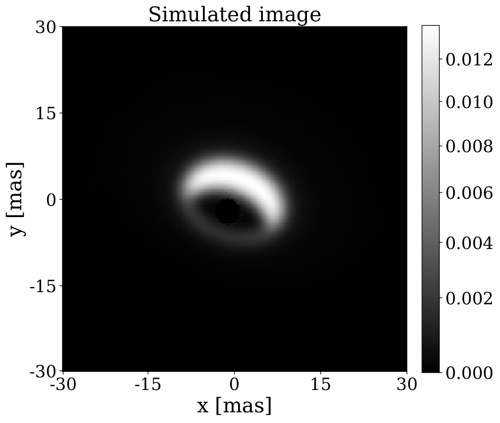

| Parameters of model 1 | Symbol | Value |
|---|---|---|
| Inner radius (au) | 5 | |
| Outer radius (au) | 1000 | |
| Truncation radius (au) | 200 | |
| Total dust mass () | ||
| Disk flaring | ||
| Radial density exponent | ||
| Scale height (au) | 20 | |
| Inclination (∘) | 42 | |
| Position angle (∘) | PA | 20 |
4.2 Fitting process
Due to the higher spatial resolution of the reconstructed -band image compared to the -band image, the former has been chosen to guide the fitting. In order to constrain the model parameters, we first analyze their impact on the inner disk structures visible in the reconstructed images. The inner radius , disk flaring , scale height at 100 au, and inclination turned out to be the most crucial parameters for the observed appearance of the innermost disk region. In contrast to this, the outer radius , truncation radius , radial density parameter , and total dust mass have hardly any impact and thus cannot be constrained. Therefore, we use parameter values which have been either constrained by former observations of the large-scale disk structure of FS CMa or can be considered as typical for this class of objects.
To quantify the goodness of the fit, we (1) calculate images of the difference between the reconstructed and simulated images. In addition, we (2) consider the absolute mean difference by averaging the absolute value of the difference images, as well as (3) the difference between observed and modeled visibilities and closure phases.
Relative flux units are used in the reconstructed images and in the simulated images. In the next step, we mask the extended image of the central star in the reconstructed -band image and in the simulated image to first focus on reproducing the brightness distribution of the disk. However, unmasked images of the simulation and reconstruction are shown later in Figs. 6 and 9. The masked simulated images are shifted within a range of a few pixels to find the best match with the reconstructed image (i.e., the minimum of the absolute mean difference). In a second step (Sect. 4.6), we compute the difference between model closure phases and observed closure phases and model visibilities with observed visibilities (called residuals below). The comparison of the total flux of the observed and simulated images is discussed in Sect. 4.4.
Inner radius and inclination
The appearance of the inner rim of the disk as seen in the -band image is mainly determined by the inner radius and disk inclination. While the inner radius directly affects the size of the inner disk cavity, the inclination determines the eccentricity of the elliptical model image (see Fig. 2, left), with potential shadowing by outer disk regions and – in interplay with the anisotropic scattering function of the dust grains – the relative contributions of forward and back-scattered radiation. Both parameters are fit simultaneously.
We constrain the inner radius by varying the inner radius between 3 au and 7 au and calculating the absolute mean difference between the reconstructed and model images by averaging the absolute value of the difference images (see Fig. 2 right) to find the best-fit image. To constrain the inclination, we perform a series of simulations for inclinations between and . These are again compared to the reconstructed image by calculating the absolute mean difference between the reconstructed and model images. Based on these simulations, we deduce first best-fit values for the inclination of and the inner radius , respectively. We note, that the temperature of the dust of the rim does not exceed 1200 K. The inner radius is therefore not perfectly corresponding to the sublimation temperature of the dust composition, which is 1300–1500 K for silicate (see, e.g., Pollack et al. 1994) and 2500 K for graphite (see, e.g., Kobayashi et al. 2011).
Scale height and flaring parameter
While the inner radius and inclination are directly related to the inner ellipse seen in the -band model, the scale height and the flaring parameter determine the radial extent of the bright inner rim. We conduct simulations with scale heights between 15 au and 30 au in steps of 5 au and compare the resulting radial extent of the inner wall with that of the reconstructed -band image. Constraining the flaring parameter is less straightforward because it affects various features in the image. Here, we have to compare the overall shape of the simulated images with the reconstructed images. To cover a sufficiently wide range of flarings, we run simulations with a flaring parameter between 0.5 and 1.5 in steps of 0.1. By increasing the flaring we increase the flux on the far side of the disk. We find that at a certain degree of flaring the disk starts to cover parts of the inner region. Considering this and excluding unrealistically high and low scale heights, we constrain the flaring parameter to 1.2 with a best-fit scale height at 100 au of around 20 au.
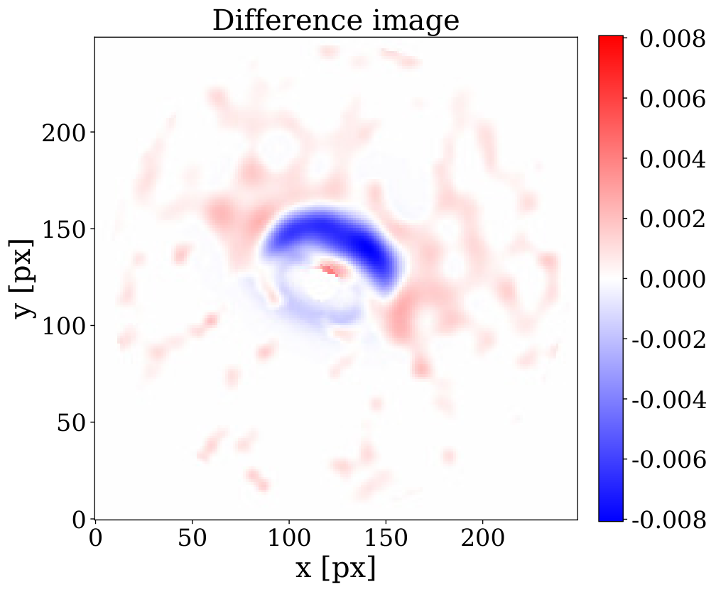
Figure 2 presents a comparison of the best-fit basic model 1 with the observed image: (from left to right) the intensity distribution of the simulated model 1 image, an overlay of the observed -band image with a contour plot of the model image, as well as the corresponding difference image (the central star is masked in the figure).
It can easily be seen that the inner elliptical gap and the extent of the bright region are well fit. However, the difference image also shows that the brightness distribution does not fit the characteristic asymmetry of the brightness distribution of the disk rim.
4.3 Modified curved inner rim (models 2 and 3)
While the basic model 1 described above allows us to roughly reproduce the shape of the image of the disk as well as the radial extent of the bright region, it is not capable of reproducing the asymmetry of the ring-like brightness distribution, as the difference image in Fig. 2 shows. Thus, the shape of the inner rim has to be modified toward a lower vertical rim extent in our model. Besides the motivation derived from our observational finding, this modification is also in agreement with previous studies based on hydrodynamical simulations and analytical considerations for the inner rim of circumstellar disks (e.g., Isella & Natta 2005, McClure et al. 2013, Flock et al. 2016). To match the brightness distribution along the inner disk rim and to take the theoretical studies into account, we expand our model by a simple parameterization of differently curved shapes of the inner rim described by the modified scale height:
| (4) |
where is the radius up to which the rim is modified, is the unmodified scale height of , and is a parameter to describe the different shapes of the inner rim. For illustration, selected examples for the different inner rim shapes are shown in Fig. 3. We now fix the best-fit parameters described in the section above and determine the best-fit of the brightness distribution of the inner rim by sampling a parameter space of (1.2–2.4) for in steps of 0.2 and 0.1–1.0 in steps of 0.1 for , respectively. The resulting map of the absolute mean difference for each model can be found in Fig. 4. In the following, we shortly discuss the impact of the two rim parameters and .


Inner rim parameter
The parameter allows us to modify the shape and therefore illumination of the inner rim of the model. As the case describes a vertical rim that extends up to with a constant height, increasing results in a worse fit (see Fig. 4). Increasing to 0.5 changes the structure of the inner rim toward a parabolic shape. This configuration does not only result in the required radially more efficient illumination of the inner disk region, but also allows the observer to see more of the inner region on the near side of the disk. Besides the qualitatively better match of the observed inner rim structure, the absolute mean difference between reconstructed and simulated images is decreasing. Values of up to 1 are describing the transition from a parabolic shape to a peaked, wedge-like inner rim, leading to an extension of the bright region to the outer parts. The corresponding simulated images show a broad, extended ring that is inconsistent with the reconstructed images.
Radius of modified inner rim
The radius of the modified inner rim describes the point up to which the basic model is modified. It is therefore directly related to the shape of the simulated image for different values of the parameter . In the case of low values of , for example, a vertical rim with constant height, an increase of results in an increasing mismatch between the simulated and reconstructed images. A similar trend can be found for high values of , which result in a bright extended ring, as described above, that increases even more when increasing . For shapes of the inner rim between parabolic and tapered, we see a decrease of the absolute difference up to a value of . This corresponds to an extension of the bright region as well as a blurring of the bright rim. Values of will not improve the model because the modified rim is extending seamlessly into the flared disk in this case, which means changes of in this regime will not influence the shape of the inner rim. Values of below 1.2 can also be neglected, because the modification of the rim would be too small to be noticed.
According to the absolute mean differences measured for the different parameter sets, we find best-fit values of and (model 2; Fig. 5). We note that the model with is deviating less than 1% from the best-fit case and is even best-fitting for larger values of . The simulated image, the contour plot as well as the plot of the differences for the best-fit case are shown in Fig. 5.


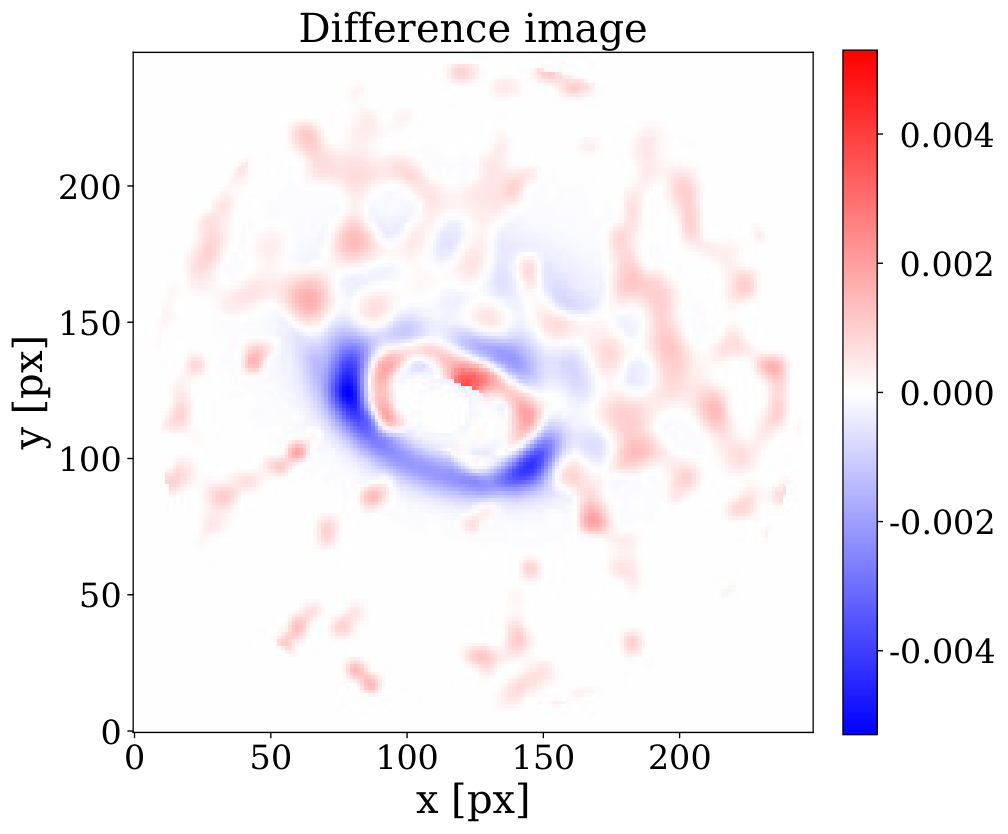
It can be seen that the difference image now has smaller values. We note that the difference plot of observed image minus model image still shows two regions with higher differences than on average. In these regions, the flux in the simulated image is higher than the measured flux on the near side.
To make sure that the modified rim is not affecting the best-fit parameters derived in Sect. 4.2, we repeat the calculations for the entire parameter grid. Comparing the differences confirms the best-fit parameters depicted in the table of Fig. 2 except for the inclination for which we now find a best-fit value of . The corresponding simulated image of this model 3, the contour plot as well as the plot of the differences are shown in Fig. 6.


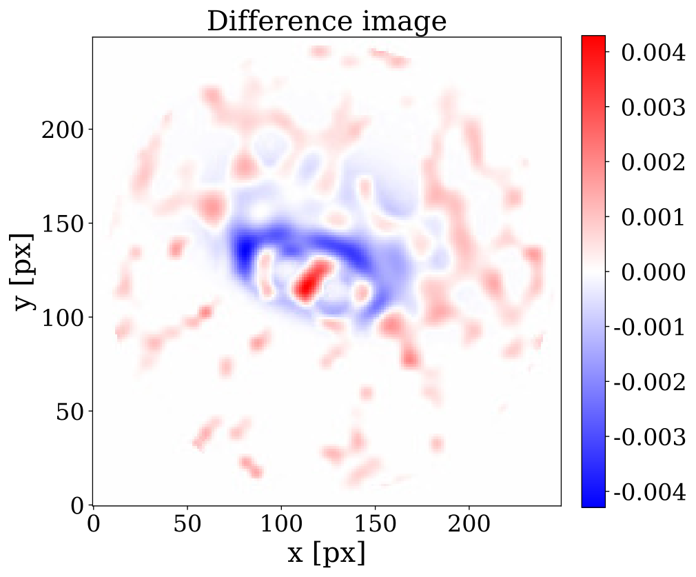
As a further check, we simulate the corresponding -band image of our model and the respective difference images. The best-fit parameter values in this case are and . In contrast to the best-fit of the reconstructed -band image, the simulated -band images with 0.7 or 0.8 are of comparable goodness, as their respective absolute mean differences are also within the measured uncertainties and are deviating by only 3%. The simulated image, contour plot and the plot of the differences between simulated and observed images of the -band best-fit parameter values are shown in Fig. 7. The best-fit parameter values derived on the basis of the reconstructed -band image fits the band equally well. As in the case of the band, the differences are on the order of the uncertainties of the reconstructed image. The trends found for the parameters describing the shape of the inner rim as depicted in Fig. 4 for the -band image can also be confirmed with the -band simulations. Thus, we consider the best-fit model 3 is consistent with the reconstructed - and -band images.


4.4 Total flux
We measure a total -band model flux of 35 Jy in the model FOV of 80 mas, while we derive an observed flux of 47 Jy (estimated uncertainty about ) from the FS CMa interferograms in their larger 0.6 arcsec FOV of the -band interferograms. The observed flux was derived by comparing the integrated flux of the interferograms of the target and the calibrator stars. In the -band, we obtain a total model flux of 110 Jy in the model FOV of 360 mas and derived an observed flux of 213 Jy () from the FS CMa -band interferograms in their FOV of 2.3 arcsec. In the model, we are thus covering about 3/4 of the observed flux in the band, but only 1/2 of the flux in the band. The differences may be caused by the flux from regions outside the model FOV.
We note that the thermal model emission always outweighs the scattered contribution by a factor of 10 in the band and a factor of 300 in the band, respectively. A detailed image of the ratio between thermal and scattered emission for both bands can be found in Fig. 8.
4.5 Model image with pure astrosilicate and a dust envelope with constant density (model 4)


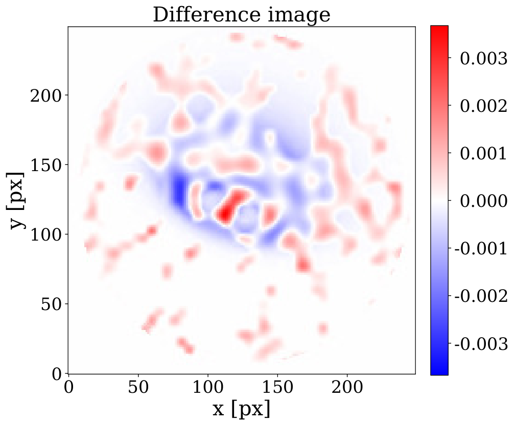
Model 3 presented in Fig. 6 in the Sect. 4.3 is able to reproduce the asymmetric structure of the inclined FS CMa disk. However, the brightness of the central object in the observed -band image and the model image disagree. In the observed -band image, the integrated -band flux of the central object is about of the total image flux, whereas in the model, the -band flux from the central object is only 0.61%.
Even though the central star shows photometric variability of more than a magnitude within years as discussed for example in de Winter & van den Ancker 1997, the stellar parameters have been well constrained by multiple previous studies (e.g., Vioque et al. 2018, Laws et al. 2020).
Increasing the luminosity of the star within the measured uncertainties will increase the flux scattered and reemitted by the disk and therefore hardly affect the star-to-disk brightness ratio. This also holds true for the effective temperature of the star which when increased, shifts the stellar emission toward shorter wavelengths, resulting in a decrease of the star-to-disk brightness ratio in the and bands.
We therefore turn our attention toward the disk properties to analyze the outlined discrepancies. The luminosity of the disk can be decreased by either reducing the illumination of the inner region or by choosing a dust mixture with different optical properties. For the first, we find that varying the flaring parameter and the scale height around the corresponding best-fit values in order to modify the disk illumination is not significantly increasing the star-to-inner rim brightness ratio. Concerning the dust properties, we conduct simulations with grain sizes up to m and find that the brightness ratio is decreasing because of an increase of the scattered radiation. Moreover, changing the dust composition to pure astronomical silicate could reduce the flux caused by dust reemission while not affecting the amount of scattered radiation and therefore reduce the brightness ratio. Corresponding simulations of our best-fit model with pure astronomical silicate show that the star-to-disk brightness ratio can be increased by a factor of 2–3 while preserving the shape of the inner rim. This finding might indicate that the dust composition is different from the assumed silicate-graphite mixture. However, it should also be noted that the measured total flux in this case is even lower and covers only a third of the observed flux.
The offset between the visibilities at low spatial frequencies of the simulated image and the observational data suggests a constant background flux that is missing in the simulated image. A very faint constant background flux would not be visible in the reconstructed image and was therefore not considered in the fitting process in Sect. 4.2 and 4.3. To account for this, we expand our disk model by adding an optically thin dust sphere with an inner radius of 5 au and an outer radius wider than the FOV of the reconstructed image. We test two simple dust density distributions for two different optical depths: a sphere with a) a constant density and b) an 1/r density profile for and . In case of the models, the simulated images show additional flux in regions that show no flux in the reconstructed images. We therefore focus on the optically thin case. Since there are no significant differences between the simulated images resulting from the two density distributions in the optically thin case (), we choose the simpler, constant density distribution for the subsequent discussion. This faint background, caused by the optically thin dust sphere, together with the assumed pure astrosilicate dust improved the fit of the model visibilities and contributed to the following new star-disk flux ratio described below. The simulated image, contour plot, and the plot of the differences between simulated and observed images of the -band best-fit model 4 with pure astrosilicate are shown in Fig. 9. In this model, the integrated flux from the central object increased from 0.61% (in the model in Fig. 6) to 1.1%, but is still smaller than the observed flux fraction. This means that model 4 with pure astrosilicate dust and an optically thin dust envelope changed the flux ratio of central object and dust disk by almost a factor of two, but the remaining flux ratio discrepancy is still a factor of four. Therefore, we discuss a more promising alternative in Sect. 4.7, the possible impact of a gaseous Be star disk.
In the previous sections, we have developed disk models that approximately agree with the observed image of the disk, but the modeled flux fraction of central object (0.61–1.1% of the total flux of central object plus dust disk) is lower than in the reconstructed image (where it is 4.5%). This disagreement may be caused by a compact gaseous disk surrounding the central star (Sect. 4.7).
Because of this gaseous disk, the central object of FS CMa seems to be much more complicated than just a normal star. This is probably the reason, why our model, which does not include a gaseous disk, is not able to reproduce the correct flux ratio of central object and dust disk. Because of this uncertainty, our main goal is only to model the shape of the dust disk. Modeling of the entire complex system of dust disk and central object is out of the scope of this paper.
In this complex situation, it became clear that the just applied modeling criterion of using the difference images of model and reconstructed images has the advantage that we can find the best-fit disk image by ignoring the reconstructed image of the central object. For this goal, we first masked the central object in previous sections before we calculated the average absolute value of the difference images to obtain an integral measure of the observation-model difference. In the next Sect. 4.6, we use another important criterion to find the best-fit image, namely the differences between modeled and observed closure phases and visibilities.
4.6 Comparison of the closure phases and visibilities derived from the model intensity distribution to the measured closure phases and visibilities
Instead of calculating the differences between reconstructed and the modeled images to constrain model parameters (as in the previous sections), we now compute the average absolute value of the difference between the observed and model visibilities and closure phases called “model-observation residuals”.
The model-observation residuals of the closure phases and the visibilities for the -band model 3 image (Fig. 6) are and 0.040, respectively. These big residuals are not surprizing because we know already from the previous sections that the model flux ratio of the central object and the disk disagrees with the observations.
These -band model-observation residuals are very big in comparison to another important type of residuals, the “reconstruction-observation” residuals, which are the residuals between the visibilities and closure phases of the reconstructed image (Fig. 1) and the observed visibilities and closure phases. The reconstruction-observation residuals are a measure of the quality of the reconstructed image. The reconstruction-observation residuals for the -band image in Fig. 1 are only and 0.009 for closure phase and visibilities, respectively (see Table 1).
One of the reasons for the big aforementioned model-observation residuals (closure phase: , visibility: 0.040) is the small flux fraction of the central object (only 0.61–1.1% of the total flux) of the models 3 and 4 (Figs. 6 and 9). Other reasons are most likely additional disk asymmetries or clumpiness, which are not included in the modeling. This strong dependence of the model-observation residuals on the too small flux fraction of the central object is problematic if we want to use the model-observation closure phase and visibility residuals to constrain the parameters of the model disk alone because these residuals depend on both the required dust disk parameters and the wrong flux ratio of central object and dust disk. We can constrain the disk parameters only if we avoid the influence of the wrong flux ratio of central model star and disk by compensating the wrong flux ratio, which can approximately be performed by applying a suitable flux scaling factor to the central model star. This scaling factor is only needed as a tool to evaluate the model-observation residuals of the disk and is not used in radiative transfer modeling. For these reasons, we first compute the dependence of the model-observation residuals on the scaling factor of the model central star. The results are shown in Figs. 10 and 11 for our two models 3 and 4 presented in Figs. 6 and 9.
Figure 10 shows the closure phase and visibility residuals of the model 3 in Fig. 6 (i.e., model-observation residuals) as a function of different scaling factors for the brightness of the model central star. The minimum closure phase residuals of are achieved with a scaling factor of 9.4. Figure 11 shows the residuals of model 4 (modified model image displayed in Fig. 9) as a function of the scaling factors. In this case, the minimum closure phase residuals of are obtained with a scaling factor of 3.9, whereas the closure phase residuals in the case of no scaling are . The remaining closure phase residuals of 25∘ are most likely caused by additional asymmetries in the dust disk, which are not taken into account in the models. This discrepancy is also shown in Fig. 24, where the measured interferometric data are plotted together with the interferometric data derived from the two models 3 and 4, but modified with the above model star scaling factors 9.4 and 3.9, respectively.
In addition to the above model-observation residual method, we used the method to determine the average deviation of the model visibilities and closure phases from the observed values. In Appendix F, we show that the method provides similar scaling factors of 9.0 and 3.7 (instead of the above 9.4 and 3.9) for the two models 3 and 4, respectively.
The model star scaling factors derived from the closure phase residuals are approximately consistent with the modeling results obtained when we used the absolute mean differences between the observed and modeled images as criterion. In this case, the model images have a flux fraction in the central object of only 0.61% (model 3) or 1.1% (model 4) of the total flux, whereas the flux fraction of the central object is (4.5 +/-0.9)% in the observed -band image, corresponding to ratio of 4.5/0.61=7.4 (model 3) and 4.5/1.1=4.1 (model 4). These model-reconstruction deviations are similar to the model central star scaling factors of 9.4 (model 3) and 3.9 (model 4) derived from the closure phase residuals.
Figure 12 shows the model-observation residuals of the -band model 3 image displayed in Fig. 7 as a function of the different scaling factors of the central star. The minimum closure phase residuals of are obtained with a central star scaling factor of 9.2, whereas the closure phase residuals in the case of no scaling are . The difference between scaling and no scaling of the central star is very small because the integrated stellar intensity is only 0.03% of the total flux of the best-fit -band model. In Fig. 26, the measured interferometric data are plotted together with the interferometric data derived from the -band reconstruction shown in Fig. 1 and derived from the model displayed in Fig. 7 (model 3), but modified with the above scaling factor 9.2.
We have shown by three different methods that the model flux ratio of the central star and the total flux (of disk and central object) is about 3–9 times too small. In Sect. 4.7 we discuss a likely cause for this discrepancy. As we discussed in previous sections, our goal is only to constrain model parameters of the dust disk. The modeling of the complex star-disk system is out of scope of this paper because of the complex central object discussed in Sect. 4.7.
Therefore, we focus now on the application of the model-observation closure phase residuals and the aforementioned results to constrain the same disk shape parameters and , which were constrained in Sect. 4.3 using the presented difference between the reconstructed image and the model image. A third required free modeling parameter is the aforementioned scaling factor of the brightness of the central star because of the derived flux ratio discrepancy.
Figure 13 shows the model-observation closure phase residuals of several versions of model 3 (i.e., – pairs with = 1.8, 2.0, 2.2 and = 0.5, 0.6, 0.7) as a function of the central star scaling factor. The best-fit models, with the smallest closure phase residuals of , have a central star scaling factor of 8.4, = 0.6, and = 1.8 and 2.2. Furthermore, the method presented in Appendix F provides the same disk parameters and as derived with the residual method applied in this section. Figures 14 and 33 show the same type of – plot as in Fig. 4, but now using the model-observation closure phase residuals or results, instead of the absolute mean differences between simulated and reconstructed images. The results of the three fits (in Figs. 4, 14, and 33) are similar. They differ in the inner rim parameter value only, 0.6 in Figs. 14 and 33 instead of 0.7 in Fig. 4. In all models presented in this study, the dust disk temperature is below the sublimation temperature. Figures 10 and 11 suggest that model 3 can reproduce the disk structure slightly better than model 4 because the closure phase residuals of model 3 at minimum scaling factor are smaller (; Fig. 10) than the closure phase residuals of model 4 (Fig. 11; ).

4.7 Influence of an additional gaseous B[e] star disk on the model brightness ratio between the central object and the dust disk of FS CMa
In the models discussed above, the model image of the central object is always too faint with respect to the dust disk. If we assume that the central star is surrounded by an additional compact (i.e., unresolved) gaseous disk, the model brightness ratio between central object (= star plus gaseous disk) and dust disk would change, as discussed below. The theory of gaseous envelopes and disks of Be stars is discussed in Lamers & Waters 1984, Waters 1986, Lee et al. 1991, Carciofi 2011, Rivinius et al. 2013, Vieira et al. 2015; Vieira et al. 2016. The gaseous disks of several Be and B[e] stars were studied with high spatial resolution using optical and infrared long-baseline interferometers (Thom et al. 1986; Mourard et al. 1989; Quirrenbach et al. 1993; Stee et al. 1995; Quirrenbach et al. 1997; Berio et al. 1999; Tycner et al. 2006; Domiciano de Souza et al. 2007; Meilland et al. 2009; Millour et al. 2011; Touhami et al. 2011; Kraus et al. 2012, e.g.,).
Below we discuss that the infrared continuum flux from a gaseous disk can be several times brighter than the stellar flux, and the brightness of the gaseous disk depends on the wavelength and the viewing angle (e.g., it is brightest for face-on viewing direction; Vieira et al. 2015; Vieira et al. 2016). Because of this viewing angle dependence, a gaseous disk can change the brightness ratio between the central object (= star plus gaseous disk) and the dust disk of FS CMa. A gaseous disk can much increase the flux from the central object seen by the observer (inclination angle 51∘). However, the illumination of the dust disk by the gaseous disk may be smaller if the gaseous and dust disk are aligned.
The dependence of the intensity ratio of total flux to stellar flux on the inclination angle, density, and wavelength can be calculated using the DISCO code (https://amhra.jmmc.fr/) based on the Vieira et al. 2015; Vieira et al. 2016 model for classical Be star gaseous disks. The stellar parameters used are given in Tab. 2. The value of the inclination angle is assumed to be 51∘, as derived during the modeling process. The parameters of the gaseous disk model are given in Tab. 3.
Figure 15 shows the dependence of the model intensity ratio of total flux (i.e., stellar plus gaseous disk flux) to the stellar flux on wavelength for different gas densities at the base of the gaseous disk and for the inclination angle of 51∘ of FS CMa. Figure 16 shows the intensity ratio of the total flux (i.e., stellar plus gaseous disk flux) to the stellar flux as a function of the wavelength for different inclination angles for a gas density at the base of the gaseous disk of 10-7 kg/m3. For example, at -band wavelengths, the total flux is about 3–4 times larger than the stellar flux for the inclination range of 0–51∘ (0∘ corresponds to face-on) of the gaseous disk in contrast to larger inclination angles. This inclination angle dependence of the brightness of such a gaseous disk would have a strong influence on the FS CMa model image if FS CMa is surrounded by a bright gaseous disk and the gaseous disk is aligned with the dust disk. In this case, the gaseous disk is seen edge-on (i.e., low brightness) from viewing locations within the dust disk, whereas we see a bright 51∘ inclined disk. Therefore, such a gaseous disk may explain the difference between the modeled and observed flux ratio of the central object and the dust disk because a gaseous disk is not taken into account in our radiative transfer modeling.
| Parameter | Value |
|---|---|
| Disk outer radius () | |
| Disk temperature (K) | |
| Density at the disk base (kg/m3) | |
| Density power law exponent | |
| Power law coefficient of disk flaring |
5 Summary and conclusions
FS CMa belongs to the subgroup of unclassified B[e] stars. It is not known whether FS CMa is a young Herbig B[e] or a star in a later evolutionary stage. Vioque et al. 2020 concluded that FS CMa is not a young star. FS CMa is famous for its large, inclined circumstellar disk and spectacular bipolar outflow perpendicular to the disk plane.
We performed aperture-synthesis imaging of FS CMa with the new VLTI-MATISSE interferometry instrument and carried out radiative transfer modeling to interpret the images. The following results were obtained:
- •
We reconstructed the first aperture-synthesis - and -band images of the stellar disk and the central object. Image reconstruction was performed with the IRBis method. The - and -band images have resolutions of 2.7 mas and 6.6 mas, respectively.
- •
In the -band image, the inner rim region of the circumstellar dust disk and the central star can be seen. The size of the resolved inner dark disk cavity is 612 mas. The resolved -band disk consists of a bright NW disk region and a much fainter SE one. The images suggest that we are looking at the bright inner wall of the NW disk rim, while the SE rim is partially self-shadowed and appears therefore dimmer in the image. Therefore, the large brightness of NW rim suggests that the NW rim is on the far side. The -band image shows only the bright NW disk region.
- •
The reconstructed images provide the basis for a detailed analysis of the disk stucture, and thus the spatial distribution of the dust in the innermost disk region. Performing radiative transfer simulations, we derived an inner disk radius of 5 au and a disk inclination of . Most importantly, the good quality of the reconstructed images, in particular the high-resolution -band image, allowed us to constrain the shape of the vertical structure of the inner few au of the inner disk. Using a parameterized disk model, the shape of the rim is described by two parameters characterizing a) the curvature of the disk rim and b) the radial range beyond which the density profile is described by the global disk model. In particular, we find a rather flat shape of the disk between the inner disk radius and 9 au. Regardless of the specific evolutionary state of FS CMa, this finding provides direct constraints for further studies of the physical mechanisms resulting in this particular shape, that is, the interaction of the stellar radiation with the gas and dust disk surrounding the central star. However, a detailed analysis taking the specifics of FS CMa into account is beyond the scope of this study.
- •
While the relative brightness distribution can be well fitted, the flux ratio between the central object and the net flux of the disk can not be matched on the basis of a star-to-dust disk model alone. Depending on the specific model setup, characterized by the chemical composition and size distribution of the dust, even taking a hypothetical envelope with a low optical depth as a source of possible contamination into account, the latter results in a star-to-disk flux ratio which is too low. All model images have a flux fraction in the central object of only 0.61–1.1% of the total flux, whereas the flux fraction of the central object is 4.5% in the observed -band image. To explain this discrepancy, we suggest the possible additional contribution of a compact gaseous B[e] star disk in the vicinity of the star. Taking the dependence of the brightness on the viewing angle into account, we find that this gaseous disk may be sufficiently bright to explain the observed flux ratio. More detailed studies of FS CMa are needed in the future to improve our understanding of its evolutionary stage, suspected companion, brightness variations, and physical properties of its suggested gaseous disk.
Acknowledgements.
MATISSE was designed, funded and built in close collaboration with ESO, by a consortium composed of institutes in France (J.-L. Lagrange Laboratory – INSU-CNRS – Côte d’Azur Observatory – University of Côte d’Azur), Germany (MPIA, MPIfR and University of Kiel), the Netherlands (NOVA and University of Leiden), and Austria (University of Vienna). We thank all ESO colleagues for the excellent collaboration. This work has been supported by the French government through the UCAJEDI Investments in the Future project managed by the National research Agency (ANR) with the reference number ANR-15-IDEX-01. The Konkoly Observatory and Cologne University have also provided some support in the manufacture of the instrument. K.O. acknowledges the support of the Agencia Nacional de Investigación y Desarrollo (ANID) through the FONDECYT Regular grant 1180066 and 1210652. S.K. und A.K. acknowledge support from an STFC Consolidated Grant (ST/V000721/1) and ERC Starting Grant (Grant Agreement No. 639889). The research of J.V. and M.H. is supported by NOVA, the Netherlands Research School for Astronomy. T.H. acknowledges support from the European Research Council under the Horizon 2020 Framework Program via the ERC Advanced Grant Origins 83 24 28. A.G. acknowledges support from the European Research Council (ERC) under the European Union’s Horizon 2020 research and innovation programme under grant agreement No 695099 (project CepBin). P.A. acknowledges support from the Hungarian NKFIH OTKA grant K132406, and from the European Research Council (ERC) under the European Union’s Horizon 2020 research and innovation programme under grant agreement No 716155 (SACCRED). J.S.B. acknowledges the support received from the UNAM PAPIIT project IA 101220 and from the CONACyT project 263975. AD thanks support from FAPESP #2019/02029-2. FN acknowledges FAPESP for support through proc. 2017/18191-8. This research has made use of the services of the ESO Science Archive Facility. This publication makes use of the SIMBAD database operated at CDS, Strasbourg, France. This research has made use of the Jean-Marie Mariotti Center (JMMC) — MOIO AMHRA service at https://amhra.jmmc.fr/. We thank the referee for helpful suggestions.References
- Baines et al. (2006) Baines, D., Oudmaijer, R. D., Porter, J. M., & Pozzo, M. 2006, MNRAS, 367, 737-753
- Berio et al. (1999) Berio, P., Stee, Ph., Vakili, F., Mourard, D., Bonneau, D., Chesneau, O., Le Mignant, D., Thureau, N., & Hirata, R. 1999, A&A, 345, 203-210
- Bjorkman & Wood (2001) Bjorkman, J. E. & Wood, K. 2001, ApJ, 554, 615
- Brunngräber et al. (2016) Brunngräber, R., Wolf, S., Ratzka, T., & Ober, F. 2016, A&A, 585, A100
- Bourges et al. (2017) Bourges, L., Mella, G., Lafrasse, S., et al. 2017, VizieR Online Data Catalog, II/346
- Byrd & Nocedal (1995) Byrd, R. H., L. P. & Nocedal, J. 1995, SIAM Journal on Scientific and Statistical Computing, 16, 1190
- Carciofi (2011) Carciofi, A. C. 2011, in Active OB Stars: Structure, Evolution, Mass Loss, and Critical Limits, ed. C. Neiner, G. Wade, G. Meynet, & G. Peters, Vol. 272, 325–336
- Chael et al. (2018) Chael, A., Johnson, M., Bouman, K., Blackburn, L., Akiyama, K., & Narayan, R. 2018, ApJ, 857, 23
- de Winter & van den Ancker (1997) de Winter, D. & van den Ancker, M. E. 1997, A&AS, 121, 275
- Domiciano de Souza et al. (2007) Domiciano de Souza, A., Driebe, T., Chesneau, O., et al. 2007, A&A, 464, 81
- Draine & Lee (1984) Draine, B. T. & Lee, H. M. 1984, ApJ, 285, 89
- Draine & Malhotra (1993) Draine, B. T. & Malhotra, S. 1993, ApJ, 414, 632
- Flock et al. (2016) Flock, M., Fromang, S., Turner, N. J., & Benisty, M. 2016, ApJ, 827, 144
- Hager & Zhang (2005) Hager, W. W. & Zhang, H. 2005, ”SIAM Journal on Optimization”, 16, 170
- Hager & Zhang (2006) Hager, W. W. & Zhang, H. 2006, SIAM J. Optim., 17, 526
- Hartmann et al. (1998) Hartmann, L., Calvet, N., Gullbring, E., & D’Alessio, P. 1998, ApJ, 495, 385
- Hofmann et al. (2014) Hofmann, K.-H., Weigelt, G., & Schertl, D. 2014, A&A, 565, A48
- Hubert & Jaschek (1998) Hubert, A. M. & Jaschek, C. 1998, B[e] stars, Vol. 233
- Isella & Natta (2005) Isella, A. & Natta, A. 2005, A&A, 438, 899
- Kenyon & Hartmann (1995) Kenyon, S. J. & Hartmann, L. 1995, ApJS, 101, 117
- Kluska et al. (2020) Kluska, J., Berger, J. P., Malbet, F., et al. 2020, A&A, 636, A116
- Kluska et al. (2014) Kluska, J., Malbet, F., Berger, J. P., et al. 2014, A&A, 564, A80
- Kobayashi et al. (2011) Kobayashi, H., Kimura, H., Watanabe, S., Yamamoto, T., & Müller, S. 2011, Earth, Planets and Space, 63, 1067-1075
- Kraus et al. (2012) Kraus, S., Monnier, J. D., Che, X., Schaefer, G., Touhami, Y., Gies, D. R., Aufdenberg, J. P., Baron, F., Thureau, N., ten Brummelaar, T. A., McAlister, H. A., Turner, N. H., Sturmann, J., & Sturmann, L. 2012, ApJ, 744, 19
- Lamers & Waters (1984) Lamers, H. J. G. L. M. & Waters, L. B. F. M. 1984, A&A, 136, 37
- Lamers et al. (1998) Lamers, H. J. G. L. M., Zickgraf, F. J., de Winter, D., Houziaux, L., & Zorec, J. 1998, A Revised Classification Scheme for B[e] Stars, ed. A. M. Hubert & C. Jaschek, Vol. 233, 277
- Laor & Draine (1993) Laor, A. & Draine, B. T. 1993, ApJ, 402, 441
- Laws et al. (2020) Laws, A. S. E., Harries, T. J., Setterholm, B. R., et al. 2020, ApJ, 888, 7
- Lazareff et al. (2017) Lazareff, B., Berger, J. P., Kluska, J., et al. 2017, A&A, 599, A85
- Lee et al. (1991) Lee, U., Osaki, Y., & Saio, H. 1991, MNRAS, 250, 432
- Lopez et al. (2014) Lopez, B., Lagarde, S., Jaffe, W., et al. 2014, The Messenger, 157, 5
- Lopez et al. (2021) Lopez, B., Lagarde, S., Petrov, R. G., et al. 2021, arXiv e-prints, arXiv:2110.15556
- Lucy (1999) Lucy, L. B. 1999, A&A, 344, 282
- Lynden-Bell & Pringle (1974) Lynden-Bell, D. & Pringle, J. E. 1974, MNRAS, 168, 603
- Mathis et al. (1977) Mathis, J. S., Rumpl, W., & Nordsieck, K. H. 1977, The Astrophysical Journal, 217, 425
- Matter et al. (2016) Matter, A., Lopez, B., Antonelli, P., et al. 2016, in Society of Photo-Optical Instrumentation Engineers (SPIE) Conference Series, Vol. 9907, Optical and Infrared Interferometry and Imaging V, ed. F. Malbet, M. J. Creech-Eakman, & P. G. Tuthill, 99070A
- McClure et al. (2013) McClure, M. K., D’Alessio, P., Calvet, N., et al. 2013, ApJ, 775, 114
- Meilland et al. (2009) Meilland, A., Stee, P., Chesneau, O., & Jones, C. 2009, A&A, 505, 687
- Menu et al. (2015) Menu, J., van Boekel, R., Henning, Th., Leinert, Ch., Waelkens, C., & Waters, L. B. F. M., 2015, A&A, 581, A107
- Millour et al. (2008) Millour, F., Petrov, R., Vannier, M., & Kraus, S., 2008, in Society of Photo-Optical Instrumentation Engineers (SPIE) Conference Series, Vol. 7013, Optical and Infrared Interferometry, M. Schöller, W.C. Danchi, & F. Delplancke, 70131G
- Millour et al. (2011) Millour, F., Meilland, A., Chesneau, O., et al. 2011, A&A, 526, A107
- Monnier et al. (2006) Monnier, J. D., Berger, J. P., Millan-Gabet, R., et al. 2006, ApJ, 647, 444
- Mourard et al. (1989) Mourard, D., Bosc, I., Labeyrie, A., Koechlin, L., & Saha, S. 1989, Nature, 342 (6249), 520-522
- Gravity Collaboration et al. (2019) Gravity Collaboration, Perraut, K., Labadie, L., Lazareff, B., Klarmann, L., Segura-Cox, D., Benisty, M., Bouvier, J., et al. 2019, A&A, 632, A53
- Petrov et al. (2018) Petrov, R. G., Allouche, F., Berio, P., et al. 2018, in Society of Photo-Optical Instrumentation Engineers (SPIE) Conference Series, Vol. 10701, Optical and Infrared Interferometry and Imaging VI, ed. M. J. Creech-Eakman, P. G. Tuthill, & A. Mérand, 1070109
- Pollack et al. (1994) Pollack, J.B., Hollenbach, D., Beckwith, S., Simonelli, D.P., Roush, T., & Fong, W. 1994, ApJ, 421, 615
- Quirrenbach et al. (1993) Quirrenbach, A., Hummel, C. A., Buscher, D. F., Armstrong, J. T., Mozurkewich, D., & Elias, N. M. 1993, ApJ, 416, L25
- Quirrenbach et al. (1997) Quirrenbach, A., Bjorkman, K. S., Bjorkman, J. E., et al. 1997, ApJ, 479, 477
- Reissl et al. (2016) Reissl, S., Wolf, S., & Brauer, R. 2016, Astronomy Astrophysics, 593, A87
- Rivinius et al. (2013) Rivinius, T., Carciofi, A. C., & Martayan, C. 2013, A&A Rev., 21, 69
- Sauter et al. (2009) Sauter, J., Wolf, S., Launhardt, R., et al. 2009, A&A, 505, 1167
- Schöller (2007) Schöller, M. 2007, New A Rev., 51, 628
- Stee et al. (1995) Stee, P., de Araujo, F. X., Vakili, F., Mourard, D., Arnold, L., Bonneau, D., Morand, F., & Tallon-Bosc, I. 1995, A&A, 300, 219
- Touhami et al. (2011) Touhami, Y., Gies, D. R., & Schaefer, G. H. 2011, ApJ, 729, 17
- Thom et al. (1986) Thom, C., Granes, P., & Vakili, F. 1986, A&A, 165, L13-L15
- Tycner et al. (2006) Tycner, C., Gilbreath, G. C., Zavala, R. T., et al. 2006, AJ, 131, 2710
- Vieira et al. (2015) Vieira, R. G., Carciofi, A. C., & Bjorkman, J. E. 2015, MNRAS, 454, 2107
- Vieira et al. (2016) Vieira, R. G., Carciofi, A. C., & Bjorkman, J. E. 2016, in Astronomical Society of the Pacific Conference Series, Vol. 506, Bright Emissaries: Be Stars as Messengers of Star-Disk Physics, ed. T. A. A. Sigut, & C. E. Jones, 135
- Vioque et al. (2018) Vioque, M., Oudmaijer, R. D., Baines, D., Mendigutía, I., & Pérez-Martínez, R. 2018, A&A, 620, A128
- Vioque et al. (2020) Vioque, M., Oudmaijer, R. D., Schreiner, M., et al. 2020, A&A, 638, A21
- Waters (1986) Waters, L. B. F. M. 1986, A&A, 162, 121
- Weingartner & Draine (2001) Weingartner, J. C. & Draine, B. T. 2001, ApJ, 548, 296
- Wolf et al. (2003) Wolf, S., Padgett, D. L., & Stapelfeldt, K. R. 2003, ApJ, 588, 373
- Zhu & Nocedal (1997) Zhu, C., B. R. H. & Nocedal, J. 1997, ACM Transactions on Mathematical Software, 23
- Zickgraf (1998) Zickgraf, F. J. 1998, Current Definition of B[e] Stars, ed. A. M. Hubert & C. Jaschek, Vol. 233, 1
Appendix A Observations
The VLTI-MATISSE observations of FS CMa are summerized in Table 4. The coverage is shown in Fig. 17. The calibrator stars used in this project are listed in Table 5.
| date | n a aa a aafootnotemark: | UT start b bb b bbfootnotemark: | UT end c cc c ccfootnotemark: | array | JD | seeing d dd d ddfootnotemark: | e ee e eefootnotemark: |
|---|---|---|---|---|---|---|---|
| 2018-12-02 | 3 | 06:25 | 08:18 | A0 B2 J2 C1 | 2458454.277 | 1.10 | 3.47 |
| 2018-12-03 | 2 | 04:00 | 05:13 | A0 B2 J2 C1 | 2458455.178 | 0.49 | 4.73 |
| 2018-12-05 | 2 | 07:14 | 07:36 | A0 B2 J2 C1 | 2458457.308 | 1.17 | 2.44 |
| 2018-12-06 | 5 | 04:00 | 08:33 | A0 B2 J2 C1 | 2458458.333 | 0.53 | 4.07 |
| 2018-12-07 | 5 | 02:44 | 07:28 | A0 B2 D0 C1 | 2458459.170 | 1.25 | 2.28 |
| 2018-12-08 | 4 | 04:33 | 08:46 | A0 B2 D0 C1 | 2458460.296 | 0.61 | 3.76 |
| 2018-12-09 | 4 | 06:06 | 09:03 | K0 B2 D0 J3 | 2458461.314 | 0.46 | 4.41 |
| 2018-12-10 | 6 | 04:48 | 08:40 | K0 G2 D0 J3 | 2458462.219 | 0.54 | 8.12 |
| 2018-12-11 | 2 | 07:23 | 08:24 | K0 G2 D0 J3 | 2458463.313 | 0.60 | 12.66 |
| 2018-12-12 | 3 | 05:07 | 08:20 | A0 G1 D0 J3 | 2458464.290 | 0.71 | 4.82 |
| 2018-12-13 | 4 | 04:58 | 08:11 | A0 G1 J2 J3 | 2458465.254 | 0.87 | 5.63 |
| 2018-12-14 | 2 | 05:17 | 06:19 | A0 G1 J2 J3 | 2458466.226 | 0.74 | 4.87 |
| 2018-12-15 | 2 | 04:52 | 07:45 | A0 G1 J2 K0 | 2458467.332 | 0.53 | 5.49 |

| name | spectral type | UDD-L a aa a aafootnotemark: | UDD-N b bb b bbfootnotemark: |
|---|---|---|---|
| 7 Cet | M1III | 5.50 0.55 mas | 5.52 0.55 mas |
| Lep | K4III | 5.87 0.56 mas | 5.92 0.56 mas |
| V407 Pup | M2Ia/ab | 2.60 0.25 mas | 2.60 0.25 mas |
| Col | K1III CN | 3.61 0.41 mas | 3.64 0.41 mas |
| Eri | M1III | 5.28 0.47 mas | 5.30 0.47 mas |
| CMa | K3/4III | 4.00 0.39 mas | 4.03 0.39 mas |
Appendix B Estimation of the visibility and closure phase errors and selection of the calibrated interferometric data
B.1 -band
Figure 18 shows examples of our obtained calibrated visibilities and closure phases (CPs). All six data sets of an observation discussed in Sect. 2.1 are displayed. To estimate the visibility and CP errors, we calculated the standard deviations of the visibilities and CPs of the six calibrated interferometric data sets of each observation (see Sect. 2.1) for each spectral channel. This is possible, because the six calibrated interferometric data sets of each observation are recorded within about 15 min, and therefore are covering nearly the same projected baseline vectors. The standard deviations were used as the common errors of the six calibrated interferometric data sets of each observation.
To obtain a reliable data set for image reconstruction, we eliminated all CPs with errors ¿ 60∘ and all visibilities with a signal-to-noise ratio ¡ 0.5. In a second selection, the reconstructed four CPs of each single observation were tested if they are affected by systematic errors. This test is called CP test and is discussed below in more detail. The four CPs measured simultaneously with a 4-telescope array are not independent, that is, each one of the four CPs can be calculated by a linear combination of the three other CPs (see, for example, Chael et al. 2018). The distance between each measured CP and the corresponding one derived from the other three simultaneously measured CPs was calculated. This distance is a linear combination of the four CP deviations (e.g., the deviation between the measured CP and its true value). In many cases this distance is small, that is, there is a good agreement between the measured CPs and the CPs derived from the three other CPs. But there may be some observations where this distance is large. The reason for this could be, for example, a nonoptimal noise bias compensation in the average bispectrum. Figure 19 shows an example observation, where the measured CPs and the CPs derived from the other three ones are very similar with respect to their noise. In Fig. 20 an observation is shown with a strong mismatch between the measured CPs and the derived CPs. In a second selection, we eliminated those observations where the mean deviation between the measured CPs and the derived CPs are larger than 8∘.
The feasibility of the aforementioned closure phase test was investigated by a computer simulation. The theoretical target was a 10 Jy source of similar structure, size, and sky position as FS CMa. The bispectrum of that target was simulated as if it were derived from data observed with the large AT configuration A0-G1-J2-K0 in -band at low spectral resolution. The bispectrum was simulated with the noise bias terms caused by the noise of a 10 Jy source and strong sky background, but without noise in the bispectrum. Figure 21 shows such a closure phase test for the simulated bispectrum with different levels of noise bias compensation (100% corresponds to perfect compensation). Because of the residulal noise bias, the reconstructed CPs systematicaly deviate from their theoretical values. The deviations between the measured CPs and the theoretical ones is zero in the case of a perfect subtraction of the noise bias term. Figure 21 shows that the distance between the measured CP and the same one derived from the three other CPs, as discussed above (e.g., the CP test, and denoted by in Fig. 21) is comparable to the distances between the measured and theoretical (true) CPs (denoted by in Fig. 21). This experiment shows that systematic errors of the CP can roughly be determined by such a CP test.
B.2 -band
The visibility and CP errors for the calibrated interferometric -band data, obtained with spectral binning of 11, were derived in the same way as in the band: the standard deviations derived from the four calibrated interferometric data sets (one for each of the four BCD configurations) of each observation (see Sect. 2.2) were calculated for each spectral channel. The derived standard deviations were used as the common errors of the four interferometric data sets of each observation.
The data set used for image reconstruction was selected in the same way as in the case of the -band data. CPs with errors ¿ 60∘ and visibilities (V2) with signal-to-noise ratio ¡ 0.5 were not used for the image reconstruction. In a second selection, the four CPs of each single observation were tested if they are affected by systematic errors. This was done with the CP test described in Appendix B.1 for the -band data. In the second selection, we eliminated all observations where the mean deviation between the measured CPs and the derived ones are larger than 1.7 the mean CP error of the corresponding observation.
Figure 22 shows examples of calibrated visibilities and CPs of a typical observation without and with different spectral binnings. The data without spectral binning (red lines) show very strong noise, which is strongly reduced by spectral binning (blue, green, and brown lines corrsponding to spectral binnings of 9, 11, and 17, respectively).
Appendix C Comparison of measured CPs and visibilities with the same ones derived from the reconstructions and from the models
Appendix D Image reconstruction
The current version of the MATISSE image reconstruction package IRBis (matcalimarec) consists of two optimization routines: a) a large-scale, bound-constrained nonlinear optimization routine called ASACG (engine 1; Hager & Zhang 2005, Hager & Zhang 2006), and b) the new built-in optimization routine, a limited memory algorithm for bound-constrained optimization called L-BFGS-B (engine 2; Byrd & Nocedal 1995, Zhu & Nocedal 1997).
The version of IRBis described in Hofmann et al. 2014 contains two cost functions: (cost fct. 1) corresponding to the function of the bispectrum, and (cost fct. 2) corresponding to the function of the bispectrum phasors plus the bispectrum moduli. denotes the current iterated image and is a two-dimensional vector in image space. The actual version of IRBis additionally contains a third cost function (cost fct. 3), which is the function of the bispectrum phasors plus the squared visibilities, given by
| (5) |
Here, and denote the measured CPs and the CPs of the current iterated image, respectively. The functions and are the errors of the bispectrum phasors and the squared visibilities, respectively. denotes the Fourier transform of the iterated image . , , and are two-dimensional spatial frequency vectors. The functions and are the point density weights of the bispecrum and the squared visibilities , respectively. The factor scales the bispectrum phasor and the squared visibilities of the iterated image to minimize the value of . The variable is the relative weight between the CP term and the squared visibility term in .
Appendix E Estimation of the error maps of the reconstructed images
In this section, we describe the building of the error maps of the reconstructed - and -band images shown in Fig. 1. For this goal, we performed computer simulations. In order to cover the noise introduced by the gaps in the coverage and by the noise in the measured data, we a) used the same coverage as the one of the MATISSE observations, and b) degraded the computed visibilities and CPs by simulated noise corresponding to the noise in the MATISSE observations, respectively. As computer simulation targets, we have chosen the models similar to those shown in Figs. 6 and 7, but with the central star intensity increased to the central star intensity of the reconstructed images in Fig. 1. The image reconstructions were performed with IRBis and the same parameters were used as for the reconstructed images shown in Fig. 1 and listed in Table 1. The error map of each of the reconstructed images (Fig. 1) is the absolute value of the difference between the computer simulation reconstruction and the computer simulation target. Before calculating the difference, the reconstruction was a) scaled to the total intensity and b) shifted to the center of the computer simulation target. To assign the reconstructions in Fig. 1 to the above produced error maps, each of the two reconstructions was a) normalized to the same total intensity as the computer simulation target, and b) shifted to the center of the computer simulation target. Figures 27 and 28 present the computer simulation experiments for deriving the error maps of the - and -band reconstructions in Fig. 1, respectively. In all four images shown in Fig. 27 (and 28), the same intensity is coded with the same color. Figures 27a and 28a are the - and -band computer simulation targets, which are convolved with point spread functions corresponding to sizes of 2.7 mas and 6.6 mas, respectively. Figures 27b and 28b present the reconstructed images obtained from the simulated data. Figures 27c and 28c show the error maps for the - and -band reconstrcutions (Fig. 1), derived from the computer simulation targets (Figs. 27a and 28a) and the computer simulation reconstructions (Figs. 27b and 28b). Finally, Figures 27d and 28d are the reconstructions shown in Fig. 1.


Appendix F Comparison of the measured CPs and visibilities with the ones derived from the model intensity distribution using the method
The model-observation values (reduced ) of the CPs and visibilities of the -band model image displayed in Fig. 6 are 738 and 1163, respectively. These big values are mainly due to the fact that the model flux ratio of the central object and the disk disagree with the observations as discussed in Sect. 4.5. These model-observation values are also very big in comparison to the reconstruction-observation values between the visibilities and CPs of the reconstructed -band image (Fig. 1 top) and the observed visibilities and CPs. The CP value is 2.88 and the visibility value is 3.97. The reconstruction-observation values of the reconstructed -band image (Fig. 1 bottom) are 1.06 for the CPs and 4.94 for the visibilities.
Figure 29 shows the CP and visibility values of model 3 (Fig. 6) as a function of different scaling factors of the model central star. The minimum CP value of 178 is achieved with a scaling factor of 9.0, which is similar to 9.4 obtained with the residual method (see Fig. 10).
Figure 30 shows values of the model 4 (Fig. 9) as a function of the scaling factors. In this case the minimum CP value of 369 is obtained with a scaling factor of 3.7, which is similar to 3.9 derived with the residual method (see Fig.11).
Figure 31 presents the CP and visibility values of the -band model image displayed in Fig. 7 as a function of the different scaling factors of the model central star. The minimum CP value of 10.6 is obtained with a scaling factor of 27, whereas the CP value in the case of no scaling is 11.0. The difference between scaling and no scaling of the central model star is very small because of its very low flux (i.e., 0.03% of the total flux of the best-fit -band model). The very low flux of the central star is responsible also for the different optimal scaling factors obtained with CP residuals (optimal scaling factor is equal to 9.2) and CP values (optimal scaling factor is 27 in this case).
Figure 32 shows the model-obseravtion CP values for several versions of model 3 (i.e., – pairs with = 1.8, 2.0, 2.2 and = 0.5, 0.6, 0.7) as a function of the central star scaling factor. The best-fit models, with the smallest CP values of 110 and 111, have a central star scaling factor of 7.8, which is similar to 8.4 obtained with the residual method (see Fig. 13), and = 0.6 and = 1.8 and 2.2, which is identical to the results of the residual method used in Sect. 4.6. For this central star scaling factor of 7.8, Fig. 33 shows the same type of – plot as in Fig. 14, but using the model-observation CP values instead of the CP residuals. The results of the two fits provide, in both cases, best-fit models with = 0.6 and = 1.8 and 2.2.
