A topology optimisation of acoustic devices based on the frequency response estimation with the Padé approximationJournal: Elsevier

Controlling sound waves in the desired manner is one of the most significant tasks in engineering. Acoustic devices to manipulate sound waves are currently designed with some trial-and-error, while the recent rapid development in computer-aided design has enabled us to exploit structural optimisation. The structural optimisation methods are classified into sizing [1], shape [2], and topology optimisations [3, 4, 5], the last of which has the highest degrees of design freedom. The topology optimisation regards structural optimisation as material distribution optimisation, which allows topological changes (e.g. creation of new holes and/or inclusions) in its process. Various researches on topology optimisation for acoustic devices are found in the literature, e.g. [6, 7]. Typically, the existing methods optimise the acoustic response to an incident wave of a single frequency. The frequency response, however, highly depends on the excitation frequency. A device optimised to a target frequency is specialised to it, and thus its performance may fall due to even a slight frequency fluctuation. When the frequency variation is expected in practical use, such a structure is not desirable. The acoustic device should exhibit excellent performance in the whole expected frequency range.

One possible approach to realise such a wide-band device is robust topology optimisation [8, 9]. In the robust topology optimisation, the (angular) frequency is regarded as a stochastic variable following the normal distribution. The frequency response becomes a stochastic variable accordingly. With these settings, one can obtain an acoustic device robust to the frequency fluctuation by letting the objective function be, for example, the weighted sum of the original objective and its standard deviation. Since it is time-consuming to evaluate the statistic quantity by the Monte-Carlo method, the deviation is often approximated through the Taylor expansion of the original objective at the mean angular frequency. We have pointed out that the high-order approximation is sometimes necessary to achieve a wide-band topology optimisation in acoustics and developed a low-cost method to evaluate the angular frequency derivatives up to an arbitrary order which is required in such a high-order approximation [9].

Another approach to realise a wide-band optimisation may define the objective function $J$ as the frequency average of the original objective $f(\omega)$ over a given frequency range $[\omega_{1},\omega_{2}]$ (target band), which is formulated as follows:

Since $f(\omega)$ is generally unknown, we need some ingenuity to evaluate the integral in Eq. (1). The simplest solution may utilise a numerical quadrature. This is, however, computationally demanding because we need to repeat the response analysis $N$ times for various excitation frequency $\omega$ to evaluate the integrand if we use a quadrature with $N$ integral points. Another solution is to replace the integrand $f(\omega)$ with its approximant. Jensen [10] proposed such a method based on the Padé approximation. In [10], $f(\omega)$ is defined as:

where $\boldsymbol{x}_{\mathrm{obs}}^{i}$, $L_{i}$, and $u$ represent the observation points, given weighting coefficient, and complex amplitude, respectively. In the evaluation of $J$ in Eq. (1), $u(\omega;\boldsymbol{x}^{i}_{\mathrm{obs}})$ is first approximated by an extended-version of the Padé approximation which can approximate $u(\omega;\boldsymbol{x}_{\mathrm{obs}}^{i})$ at all the observation points $\boldsymbol{x}_{\mathrm{obs}}^{i}~(i=1,\cdots,N_{\mathrm{obs}})$ simultaneously. The approximant for $u(\omega;\boldsymbol{x}_{\mathrm{obs}}^{i})$ is then used to form an approximation of $f(\omega)$, which is integrated by a numerical quadrature to evaluate (the approximation of) $J$. Note that the frequency range where such an approximation for $f$ holds is limited to a certain range around the approximation centre $\omega_{0}$. In the case that a single Padé approximation cannot cover the entire target band $[\omega_{1},\omega_{2}]$, the band is divided into several subintervals in each of which the approximation is applied. In [10], the number of the subintervals is given a priori.

The Padé approximation uses the following rational function:

to approximate a function $g(z)$ around $z_{0}$, in which $g:\mathbb{C}\rightarrow\mathbb{C}$ is generally a complex-valued function, and $p_{i}~(i=0,\cdots,M)$ and $q_{i}~(i=0,\cdots,N)\in\mathbb{C}$ are the coefficients. We call the rational function $g_{[M,N]}$ as “$[M,N]$ Padé approximation” of $g$ in this paper. The coefficients $p_{i}$ and $q_{i}$ are determined such that the approximated rational polynomial $g_{[M,N]}(z)$ has the same Taylor expansion at $z_{0}$ as the original function $g(z)$ up to $(M+N)$-th order. The most important advantage of the Padé approximation is that it can beyond the Taylor expansion’s radius of convergence. The frequency response function $u(\omega;\boldsymbol{x}_{\mathrm{obs}}^{i})$ may have some poles corresponding to the eigenfrequencies, and the radius of convergence is determined by the distance from the expansion centre to the nearest pole. The frequency range where the Taylor expansion is valid can thus be very narrow. This is exactly why the rational polynomial instead of the standard polynomial is used in [10]. It is shown that the strategy may work even for a practical design in automobile industry [7].

This paper aims to extend the Padé-based topology optimisation to manipulate acoustic scattering in an unbounded region, which is of great interest in engineering because many acoustic devices (e.g. sound-proofing wall) operate in the infinite domain. We adopt the boundary element method (BEM) instead of the standard finite element method (FEM) in the objective and sensitivity computations. This choice is motivated by the fact that BEM requires fewer elements than FEM in the scattering analysis. Besides, we can deal with the boundary condition at the infinity in a strict manner by BEM without any artificial boundary. In addition to the extension, we shall address improving the original Padé-based topology optimisation in two ways. Firstly, we propose to avoid the numerical integration to evaluate the frequency integral of the Padé-approximated response. To use the numerical quadrature for the rational polynomial, one needs to carefully choose the quadrature rule since the rational polynomial may have some poles. Otherwise, the result can be inaccurate. It is also difficult to set in advance the appropriate number of integral points. We propose a drastic solution to these issues, i.e. derive the analytical expression for the objective function written by the integral of the rational polynomial approximation. We also present the analytical expression for its topological derivative. Furthermore, we provide an efficient numerical algorithm to compute the ingredients of the quantities. Secondly, we propose a simple adaptive strategy to subdivide the integral range in the case that we cannot accurately evaluate the objective with a single Padé approximation.

The rest of this paper is organised as follows. In Section 2, we formulate the boundary value problem governing the scattering problem and the related structural optimisation problem. In Section 3, we derive the approximations of the frequency average based on the Padé approximation. We propose two approximations and compare their performances numerically in Section 4. In Sections 5 and 6 we review the way to evaluate the angular frequency derivatives, which is required to obtain the Padé approximation. In Section 7, we derive the topological derivative of the objective function. In Section 8, we propose a simple method to divide the target band into the appropriate number of subintervals. In Section 9, we show some validation results and examples of optimised acoustic designs. Finally, we conclude this paper in Section 10.

In this section, we define the boundary value problem and the structural optimisation problem of interest.

We consider a two-dimensional acoustic scattering caused by acoustically rigid material as shown in Fig. 1. We assume that the sound pressure $u^{*}$ oscillates time-harmonically as $u^{*}(\boldsymbol{x},t)=\Re\left[u(\boldsymbol{x})\mathrm{e}^{-\mathrm{i}\omega t}\right]$ where $\boldsymbol{x}$, $t$, $u$, and $\omega$ denote the position, time, complex sound pressure, and angular frequency, respectively. $\Re$ denotes the real part of a complex number. In Fig. 1, $u_{\mathrm{in}}(\boldsymbol{x})$ is the incident wave with which the scattered wave is defined as $u_{\mathrm{sc}}(\boldsymbol{x}):=u(\boldsymbol{x})-u_{\mathrm{in}}(\boldsymbol{x})$. $u(\boldsymbol{x})$ satisfies the two-dimensional Helmholtz equation (4) and the Neumann boundary condition Eq. (5) on the scatterer surface $\Gamma$, and the scattered wave $u_{\mathrm{sc}}(\boldsymbol{x})$ satisfies the outgoing radiation condition Eq. (6) as follows:

where $c$ and $\frac{\partial}{\partial n}$ denote the wave velocity in $\Omega$ and the normal direction derivative, respectively. The normal vector $\boldsymbol{n}$ on $\Gamma$ is directed inward to the rigid material.

Next, we define the objective function $J$ in the structural optimisation problem. $N_{\mathrm{obs}}$ observation points $\boldsymbol{x}_{\mathrm{obs}}^{i}$ are introduced in the fluid domain $\Omega$, with which the objective function $J$ is defined as follows:

where $[\omega_{1},\omega_{2}]$ is the target band in which the optimised acoustic device will be used. $J$ in Eq. (7) physically indicates the sound intensity averaged over the frequency band $[\omega_{1},\omega_{2}]$ and the observation points $\boldsymbol{x}_{\mathrm{obs}}^{1},\ldots,\boldsymbol{x}_{\mathrm{obs}}^{N_{\mathrm{obs}}}$, where $\omega_{1}$, $\omega_{2}$, and $\boldsymbol{x}_{\mathrm{obs}}^{i}\;(i=1,\ldots,N_{\mathrm{obs}})$ are given by users according to their purpose. In Eq. (8), we explicitly list $\omega$ as the argument of $u$ to emphasise that $u$ is a function of the angular frequency. To solve the structural optimisation problem optimising $J$ in Eq. (7) under the constraints Eqs. (4)–(6) and $\mathbb{R}^{2}\backslash\overline{\Omega}\subset D$, where $D\subset\mathbb{R}^{2}$ is a bounded domain called fixed design domain, we use a topology optimisation method with the level-sets of a B-spline surface [5]. To make the paper self-contained, we give a brief description of the method in A.

In this section, we describe numerical methods to evaluate the objective function $J$ in Eq. (7). Since the integrand $f(\omega)$ cannot generally be written explicitly as a function of $\omega$, the approximate function of $f(\omega)$ is used instead of $f(\omega)$ itself. Here, we may have two possibilities in the approximation; one is to apply the Padé approximation directly to $f(\omega)$, while the other is to $u(\omega;\boldsymbol{x}_{\mathrm{obs}}^{i})$ on each observation point $\boldsymbol{x}_{\mathrm{obs}}^{i}$ with which the approximation of $f(\omega)$ is obtained.

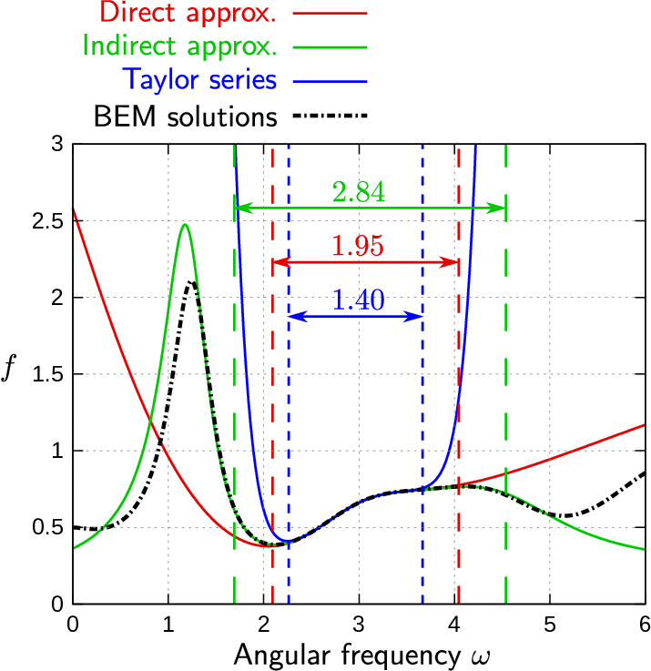
In this section, we demonstrate which of the direct or indirect approximation methods are better in approximating the frequency-dependent objective function $f(\omega)$. Let us consider the two-dimensional scattering problem as shown in Fig. 2. Four rigid scatterers, each of which is discretised into 100 boundary elements, are arranged around the origin at which the observation point is placed. The incident wave is the plane wave with the wave velocity $c=1.0$ and unit amplitude propagating along the $x_{2}$-axis. Figure 3 shows the approximation curves of $f(\omega)$ obtained by the direct and indirect approximation methods with $[4,4]$ Padé approximation at $\omega_{0}=3.0$. For reference, the values of $f(\omega)$ evaluated by the BEM for various $\omega$ in the range (“BEM solutions”) and the Taylor series of $f(\omega)$ at $\omega_{0}=3.0$ truncated at the 8th order (“Taylor series”) are also plotted in Fig. 3. A pair of the same coloured dashed vertical lines show the range where the absolute error in the approximation to “BEM solutions” is less than 0.01. We can see that the indirect approximation method can approximate $f(\omega)$ in the widest region. The direct approximation method is superior to the Taylor expansion while inferior to the indirect approximation method. Figure 4 shows the relationship between the highest order of the angular frequency derivative and the range width where the absolute error is less than 0.01. The order of the Padé approximation is chosen such that $M$ and $N$ are identical to each other. The indirect approximation method most rapidly converges to $f(\omega)$. Based on Figs. 3 and 4, we conclude that the indirect approximation method is better in approximating $f(\omega)$ and henceforth use this method.

The angular frequency derivatives $u^{(n)}:=\mathrm{d}^{n}u/\mathrm{d}\omega^{n}$ are required to obtain the Padé approximation of the angular frequency response. We have already established a low-cost method to compute $u^{(n)}$ [9], which is briefly reviewed in this section. Equations (4)–(6) with the angular frequency $\omega_{0}$ are equivalent to the following boundary integral equation (BIE):

where $\frac{\partial}{\partial n_{y}}$ and $\int_{\Gamma}\cdot\>\mathrm{d}\Gamma_{y}$ denote the normal derivative and boundary integral on $\Gamma$ with respect to $\boldsymbol{y}$, respectively. Also, $G(\boldsymbol{x},\boldsymbol{y})$ is the following Green function of the two-dimensional Helmholtz equation:

that satisfies the outgoing radiation condition Eq. (6), where $H^{(1)}_{0}$ is the Hankel function of the first kind and zeroth order. The piecewise constant elements and collocation method, for example, give one numerical solution of Eq. (23). The solution of Eq. (23) may, however, be polluted by the so-called fictitious eigenfrequency [12]. An alternative BIE free from it is well-established as

where p.f. indicates the finite part of the diverging integral, and the kernel function $W$ is defined as

where $\gamma$ is a complex constant whose imaginary part is non-zero and is set as $\gamma=-\mathrm{i}c/\omega_{0}$. $q_{\mathrm{in}}$ denotes the normal derivative of $u_{\mathrm{in}}$. The BIE (25) is called the Burton-Miller type. By differentiating Eq. (25) with respect to angular frequency $n$ times, we obtain the following boundary integral equation:

We can obtain $u^{(0)}(=u)$ by solving Eq. (25) and recursively solve Eq. (27) from $n=1$ to the highest ($=(M+N)$-th in this paper) derivative in order. By solving Eqs. (25) and (27) at $\omega=\omega_{0}$, we can compute the boundary values of $u(\boldsymbol{x};\omega_{0})$ and $u^{(n)}(\boldsymbol{x};\omega_{0})$. The forward mode automatic differentiation [9] is available to compute the higher-order angular frequency derivatives of $W$, $u_{\mathrm{in}}$ and $q_{\mathrm{in}}$ in Eq. (27). All the linear equations obtained by the discretised Eq. (27) share the identical LHS matrix for all $n$. It is, therefore, reasonable to use a direct solver, such as the LU factorisation, to solve them. We use the hierarchical matrix method [13] to efficiently assemble the LHS and LU factorise it.

The objective function $J$ and its sensitivity (to be discussed in Section 7) are evaluated via $u(\boldsymbol{x})$ and $u^{(n)}(\boldsymbol{x})$ $\boldsymbol{x}\in\Omega$, which is obtained by the following integral representation:

and its $n$-th angular frequency derivatives. The automatic differentiation is again engaged to evaluate them.

The RHS of Eq. (27) involves the layer potential whose kernels are the angular frequency derivatives of the Green function. It is quite time-consuming to compute them naively with the automatic differentiation. We can accelerate such computations by the fast multipole method (FMM) [14, 15] with minor modifications. Note that this also applies to the angular frequency derivatives of Eq. (28). We first introduce an auxiliary frequency-dependent variable $v$ defined as

The boundary integrals in the RHS of Eq. (27) is then rewritten as follows:

Since the representation in the parentheses of Eq. (30) is nothing but a usual layer potential (see Eq. (25)), we can use the standard FMM to compute it. Furthermore, the automatic differentiation provides its angular frequency derivatives simultaneously. Thus, we just need to install the automatic differentiation routine in an existing FMM code. We here summarise the formulas of the low-frequency FMM used in this study.
The multipole moment:

in which $\Gamma_{s}$ is a part of the boundary $\Gamma$.
M2M formula:

M2L formula:

L2L formula:

The local expansion:

In the above formulas, $I_{n}$ and $O_{n}$ are the solutions of the Helmholtz equation in $\mathbb{R}^{2}$ whose explicit representations are given as

where $(r,\theta)$ is the polar coordinate of $\boldsymbol{x}$, and $J_{n}$ is the Bessel function of $n$-th order. Note that $I_{n}$, $O_{n}$, $M_{n}$, and $L_{n}$ are frequency-dependent and thus their angular frequency derivatives must be computed. They are, however, computed “automatically” with the help of the automatic differentiation. In Eqs. (32)–(34), the infinite sums are truncated at a finite order. We have numerically confirmed that we can determine the truncation order in a standard way [16] with the standard FMM for the two-dimensional Helmholtz equation.

In this section, we discuss the computation of the design sensitivity. We adopt the topological derivative of the objective function as the design sensitivity. In this paper, $[\mathcal{D}_{\mathrm{T}}g](\boldsymbol{x})$ denotes the topological derivative of $g$. Let us assume that a small rigid circular scatterer of radius $\varepsilon>0$ is introduced to $\boldsymbol{x}\in\Omega$, and a variable $g$ changes to $g+\delta g(\boldsymbol{x};\varepsilon)$ due to the topological perturbation. In this case, the topological derivative $\mathcal{D}_{\mathrm{T}}g$ is defined by the following limit:

In our method, the objective function $J$ is computed by the indirect approximation method as Eq. (20). Its sensitivity is also computed based on this approximation. In this section, we show the formulation in the case of $N_{\mathrm{obs}}=1$ and discuss the case of $N_{\mathrm{obs}}>1$ later. The procedure to derive $\mathcal{D}_{\mathrm{T}}J$ is as follows: first, the topological derivatives $[\mathcal{D}_{\mathrm{T}}u_{\mathrm{obs}}](\boldsymbol{x})$ and $[\mathcal{D}_{\mathrm{T}}u_{\mathrm{obs}}^{(n)}](\boldsymbol{x})$, where $u_{\mathrm{obs}}:=u(\boldsymbol{x}_{\mathrm{obs}},\omega_{0})$ is introduced, are computed. Then, $\mathcal{D}_{\mathrm{T}}J$ shall accordingly be derived by the chain rule.

References

- [1] W. Prager, A note on discretized Michell structures, Computer Methods in Applied Mechanics and Engineering 3 (3) (1974) 349–355.
- [2] T. Takahashi, D. Sato, H. Isakari, T. Matsumoto, A shape optimisation with the isogeometric boundary element method and adjoint variable method for the three-dimensional Helmholtz equation, Computer-Aided Design 142 (2022) 103126.
- [3] M. Bendsøe, N. Kikuchi, Generating optimal topologies in structural design using a homogenization method, Computer Methods in Applied Mechanics and Engineering 71 (2) (1988) 197–224.
- [4] S. Amstutz, H. Andrä, A new algorithm for topology optimization using a level-set method, Journal of Computational Physics 216 (2) (2006) 573–588.
- [5] H. Isakari, T. Takahashi, T. Matsumoto, A topology optimization with level-sets of B-spline surface, Transactions of JASCOME 17 (2017) 125–130.
- [6] E. Wadbro, M. Berggren, Topology optimization of an acoustic horn, Computer Methods in Applied Mechanics and Engineering 196 (1-3) (2006) 420–436.
- [7] J. Kook, J. S. Jensen, S. Wang, Acoustical topology optimization of Zwicker’s loudness with Padé approximation, Computer Methods in Applied Mechanics and Engineering 255 (2013) 40–66.
- [8] Y. Sato, K. Izui, T. Yamada, S. Nishiwaki, Robust topology optimization of optical cloaks under uncertainties in wave number and angle of incident wave, International Journal for Numerical Methods in Engineering 121 (17) (2020) 3926–3954.
- [9] J. Qin, H. Isakari, K. Taji, T. Takahashi, T. Matsumoto, A robust topology optimization for enlarging working bandwidth of acoustic devices, International Journal for Numerical Methods in Engineering 122 (11) (2021) 2694–2711.
- [10] J. S. Jensen, Topology optimization of dynamics problems with Padé approximants, International Journal for Numerical Methods in Engineering 72 (13) (2007) 1605–1630.
- [11] O. Aberth, Iteration methods for finding all zeros of a polynomial simultaneously, Mathematics of Computation 27 (122) (1973) 339–344.
- [12] A. J. Burton, G. F. Miller, The application of integral equation methods to the numerical solution of some exterior boundary-value problems, Proceedings of the Royal Society of London. A. Mathematical and Physical Sciences 323 (1553) (1971) 201–210.
- [13] M. Bebendorf, Hierarchical matrices, Springer, 2008.
- [14] V. Rokhlin, Rapid solution of integral equations of classical potential theory, Journal of Computational Physics 60 (2) (1985) 187–207.
- [15] L. Greengard, V. Rokhlin, A fast algorithm for particle simulations, Journal of Computational Physics 73 (2) (1987) 325–348.
- [16] R. Coifman, V. Rokhlin, S. Wandzura, The fast multipole method for the wave equation: A pedestrian prescription, IEEE Antennas and Propagation magazine 35 (3) (1993) 7–12.
- [17] A. Carpio, M. L. Rapún, Solving inhomogeneous inverse problems by topological derivative methods, Inverse Problems 24 (4) (2008) 045014.
- [18] T. Yamada, K. Izui, S. Nishiwaki, A. Takezawa, A topology optimization method based on the level set method incorporating a fictitious interface energy, Computer Methods in Applied Mechanics and Engineering 199 (45-48) (2010) 2876–2891.
- [19] Y. Saad, M. H. Schultz, GMRES: A generalized minimal residual algorithm for solving nonsymmetric linear systems, SIAM Journal on Scientific and Statistical Computing 7 (3) (1986) 856–869.
Appendix A Level-set method with B-spline surface
In this section, a topology optimisation method with the level-set of a B-spline surface [5] is reviewed, which is used to solve the structural optimisation problem. The use of this method is not essential, and other solvers such as [18] are also available.
In the level-set method, a scalar function called the level-set function is introduced to represent the material distribution in the design domain , which is defined as