Positron Position Operators. I.
A Natural Option

In the standard representation of vectors from the Hilbert space of the free Dirac quantum field, they can be written as wave functions $\psi$ of the positions of a variable number of particles; the associated $|\psi|^{2}$ distribution over particle position configurations corresponds to position operators that I call the obvious position operators. In this paper I suggest that the obvious position operators are not physically correct and introduce instead a different set of position operators that is more closely linked to the position variable $\boldsymbol{x}$ in the field operators $\Psi_{s}(\boldsymbol{x})$ and to what is called the local observables in algebraic quantum field theory.

I begin by making explicit the obvious position operators, then I will say something about why it is desirable to have position operators at all, and then, in Sections 2–9, I will introduce and discuss the new proposal. I discuss another possibility in [38].

The definition of $P_{\mathrm{nat}}$ is based on charge operators $Q(A)$ associated with regions $A$ in 3-space, which are in turn defined in terms of the field operators $\Psi_{s}(\boldsymbol{x})$. To make their definition explicit, we abbreviate $(\boldsymbol{x},s)$ by $x$ and recall the standard definition [37] of the electron/positron annihilation/creation operators: for $f\in\mathscr{H}_{1+}$ and $g\in\mathscr{H}_{1-}$,

Then, for $f\in\mathscr{H}_{1}$, the field operator is (e.g., [34, 3, 33])

where $P_{1\pm}$ is the projection $\mathscr{H}_{1}\to\mathscr{H}_{1\pm}$. The field operators satisfy canonical anti-commutation relations (CAR) for $f_{1},f_{2}\in\mathscr{H}_{1}$,

The expression $\Psi_{s}(\boldsymbol{x})$ can then be understood as an operator-valued distribution.

The charge operators $Q(A)$ for $A\subseteq\mathbb{R}^{3}$ are then defined as

where the colons mean normal ordering, which amounts here merely to the addition of an infinite constant $c$. (The sign in front of the integral reflects the fact that the charge of the electron is negative.) The charge operators are apparently self-adjoint with spectrum $\mathbb{Z}$, $\sigma$-additive, i.e.,

and commute with each other by virtue of the CAR (23),

By the spectral theorem, they can be diagonalized simultaneously.

A point in the joint spectrum provides an eigenvalue $q(A)$ of $Q(A)$ for every $A\subseteq\mathbb{R}^{3}$, and thus an integer-valued set function $A\mapsto q(A)$ that inherits the additivity from the $Q(A)$ (because for a joint eigenvector of two operators $Q_{1},Q_{2}$, the eigenvalue of the sum $Q_{1}+Q_{2}$ is the sum of the eigenvalues).

This means the following. A set function $A\mapsto q(A)$ is locally bounded if for every $\boldsymbol{x}\in\mathbb{R}^{3}$ there is a radius $r>0$ and a (finite) $C>0$ such that for all $A\subseteq B_{r}(\boldsymbol{x})=\{\boldsymbol{y}\in\mathbb{R}^{3}:|\boldsymbol{y}-\boldsymbol{x}|<r\}$,

Here is how an integer-valued, additive set function $q(\cdot)$ can fail to be locally bounded: suppose $A_{0}$ is a brick (3d rectangle) with (say) $q(A_{0})=0$ that can be subdivided into two smaller bricks, $A_{0}=A_{1}\cup A^{\prime}_{1}$, such that $q(A_{1})=1$ and $q(A^{\prime}_{1})=-1$; suppose $A_{1}$ can be further subdivided into two smaller bricks, $A_{1}=A_{2}\cup A^{\prime}_{2}$, such that $q(A_{2})=2$ and $q(A^{\prime}_{2})=-1$; and so on, $A_{k}=A_{k+1}\cup A^{\prime}_{k+1}$ such that $q(A_{k})=k$ and $q(A^{\prime}_{k})=-1$. Obviously, the $q(A_{k})$ are unbounded while all $A_{k}$ are contained in $A_{0}$ and thus in some ball.

It also follows that the $A^{\prime}_{k}$ are mutually disjoint, so $q(A^{\prime}_{1}\cup A^{\prime}_{2}\cup\ldots)$, which must be a (finite) integer, cannot agree with $q(A^{\prime}_{1})+q(A^{\prime}_{2})+\ldots=-\infty$, so $q(\cdot)$ cannot be $\sigma$-additive, while it can be finitely additive. In fact, Conjecture 1 can equivalently be reformulated by saying that the joint spectrum consists (up to $P_{\mathrm{nat}}$-null sets) of locally $\sigma$-additive functions $q(A)$.³³ 3 It may seem strange that $\sigma$-additivity would locally be inherited but not globally. Why would that be? It may be because wave functions tend to 0 at infinity.

Now locally bounded, additive set functions are of the form

for every bounded set $A$, where $S$ is a locally finite subset of $\mathbb{R}^{3}$ and $q_{\boldsymbol{x}}$ an integer (the charge at $\boldsymbol{x}$). In other words, if the charge content of $A$ is locally bounded, then there are only locally finitely many charges. Since it is an event of measure zero for two charges to be at the same location, we can assume as well that $q_{\boldsymbol{x}}=\pm 1$. That is, for a point in the joint spectrum given by the set function $q(\cdot)$, there is a locally finite set $S_{+}$ of positive charges and a locally finite set $S_{-}$ of negative charges so that

for every bounded set $A\subseteq\mathbb{R}^{3}$. So, a configuration can be specified by specifying $S_{-}$ and $S_{+}$; correspondingly, $P_{\mathrm{nat}}$ is a PVM on

with

the space of locally finite configurations.

Plausibly, our universe is approximately a 3-sphere and thus has finite 3-volume. Finite 3-volume makes $P_{\mathrm{nat}}$ easier to treat, as then configurations are finite.

As a concrete model with finite 3-volume, let us consider instead of $\mathbb{R}^{3}$ a box $[0,L)^{3}$ of side length $L$, and

with periodic boundary conditions, so that space can be regarded as a 3-torus $\mathbb{T}^{3}$ of period length $L$. Define $\mathscr{H}_{1}=L^{2}(\mathbb{T}^{3},\mathbb{C}^{4})$, $\mathscr{H}_{1\pm}$ as the positive (negative) spectral subspace of $H_{1}$, $\mathscr{H}=\mathscr{F}(\mathscr{H}_{1+})\otimes\mathscr{F}(C\mathscr{H}_{1-})$, $\Psi_{s}(\boldsymbol{x})$, $Q(A)$ for $A\subseteq\mathbb{T}^{3}$, and $P_{\mathrm{nat}}$ as before. Conjecture 1 then implies that $P_{\mathrm{nat}}$ is concentrated on the finite configurations (see Figure 1), i.e., it is a PVM on

I propose an ontology, corresponding to this configuration space, with a variable but finite number of point particles that come in two kinds called electrons and positrons. The Born rule then says that their configuration is distributed according to

I will discuss the possibility of Bohmian trajectories for them in Section 7.3. We will see that $P_{\mathrm{nat}}$ is unusual in that its vacuum subspace, the range of $P_{\mathrm{nat}}(\{\emptyset\})$, has infinite dimension rather than dimension 1.

It is useful to see how $P_{\mathrm{nat}}$ arises in the continuum limit of a discrete space. To this end, consider, instead of $\mathbb{R}^{3}$ or $\mathbb{T}^{3}$, a discrete version of $\mathbb{T}^{3}$ in the form of the finite lattice (see Figure 2)

with $N^{3}$ sites.

Let the 1-particle Hamiltonian be

with $\nabla$ the difference operator,

and periodic boundaries. The 1-particle Hilbert space $\mathscr{H}_{1}=L^{2}(\mathcal{L},\mathbb{C}^{4})$ has dimension $4N^{3}$ while the Fock space $\mathscr{H}=\mathscr{F}(\mathscr{H}_{1})$ has dimension $16^{N^{3}}$. The latter can be regarded as the tensor product

where

Decomposing the latter Fock space into sectors by particle number yields

In this setting, $\Psi_{s}(\boldsymbol{x})$ is literally the annihilation operator and $\Psi^{\dagger}_{s}(\boldsymbol{x})$ literally the creation operator.

An element $\psi$ of $\mathscr{F}(\mathscr{H}_{1})$ can be written as a function of a variable number $\ell$ of particles, $\psi=\psi^{\ell}_{s_{1}...s_{\ell}}(\boldsymbol{x}_{1}\ldots\boldsymbol{x}_{\ell})$, so $|\psi|^{2}$ defines a probability distribution over the configuration space

as unordered configurations can be specified by specifying the occupation number for each lattice site, and the maximum occupation number is 4 due to fermionic symmetry and the dimension 4 of the spin space $\mathbb{C}^{4}$; see Figure 3 for an example of a configuration from $\mathcal{Q}_{N}$.

Let me introduce some terminology. I call the “particles” in this configuration pre-particles because in my proposal they are not ontologically the real particles. I call the associated PVM $P_{\mathrm{pre}}$; it is a PVM on $\mathcal{Q}_{N}$ acting on $\mathscr{H}$; in fact, $\mathscr{H}$ can be regarded as a subspace of $\mathscr{K}=L^{2}(\mathcal{Q}_{N},\mathscr{C})$ with $\mathscr{C}=\oplus_{n=0}^{4N^{3}}(\mathbb{C}^{4})^{\otimes n}$, and

The bottom configuration is the unique configuration with 0 pre-particles. The bottom state $|B\rangle$ is the unique (up to phase) unit vector in $\mathscr{H}$ that has 0 pre-particles. The level configuration $q_{\mathscr{L}}$ is the unique configuration with 2 pre-particles at each lattice site (see Figure 4).

A level state is a vector in $\mathscr{H}$ concentrated on the level configuration. Level space $\mathscr{L}$ is the set of all level states; it is a subspace of $\mathscr{H}$ given by

Its dimension is $6^{N^{3}}$. Here is what $\mathscr{L}$ looks like: Let $\{e_{1},e_{2},e_{3},e_{4}\}$ denote the canonical orthonormal basis of $\mathbb{C}^{4}$ and $|ij\rangle:=e_{i}\wedge e_{j}$. Then $\{|12\rangle,|13\rangle,|14\rangle,|23\rangle,|24\rangle,|34\rangle\}$ is an orthonormal basis of $\mathscr{F}_{2}(\mathbb{C}^{4})$, and

is an orthonormal basis of $\mathscr{L}$; an example of a choice of $i_{\boldsymbol{x}}$ and $j_{\boldsymbol{x}}$ for every $\boldsymbol{x}\in\mathcal{L}$ is shown in Figure 5.

The sea state is $|\Omega\rangle=\varphi_{1}\wedge\varphi_{2}\wedge\cdots\wedge\varphi_{2N^{3}}$ (up to phase) with $\{\varphi_{1},\varphi_{2},\ldots,\varphi_{2N^{3}}\}$ any orthonormal basis of the negative spectral subspace $\mathscr{H}_{1-}$ of $H_{1}$. The sea state is not level, $|\Omega\rangle\notin\mathscr{L}$. It is an eigenstate of $\Psi^{\dagger}(\varphi_{k})\Psi(\varphi_{k})$, but not of $\Psi_{s}^{\dagger}(\boldsymbol{x})\Psi_{s}(\boldsymbol{x})$.

I can now define the analog $P_{{\mathrm{nat}},N}$ of $P_{\mathrm{nat}}$ for the lattice case. On a discrete space (such as $\mathcal{Q}_{N}$), a PVM can be specified by specifying it for each point. $P_{{\mathrm{nat}},N}$ arises from $P_{\mathrm{pre}}$ by a re-interpretation as in Figure 6: 2 pre-particles are regarded as 0 electrons and 0 positrons, 3 pre-particles as 1 electron and 0 positrons, 4 pre-particles as 2 electrons and 0 positrons, 1 pre-particle as 0 electrons and 1 positron, and 0 pre-particles as 0 electrons and 2 positrons.

Note that range $P_{{\mathrm{nat}},N}(\{\emptyset\})=\mathscr{L}$, so the “vacuum subspace” according to $P_{\mathrm{nat}}$ has large dimension. We obtain $P_{\mathrm{nat}}$ from $P_{{\mathrm{nat}},N}$ in the continuum limit $N\to\infty$ while keeping $L$ fixed, so that $\mathcal{L}$ approaches $\mathbb{T}^{3}$, while considering only states that differ from $|\Omega\rangle$ by finitely many pre-particles. Conjecture 1 then implies that

while

Several authors [5, 8, 10] have proposed, specifically in the context of Bohmian mechanics, that the Dirac sea should be taken literally in the sense that positrons do not exist as particles in their own right, whereas electrons of positive or negative energy do; a situation that we normally regard as vacuum would then not only have a quantum state $|\Omega\rangle$ that in some mathematical sense involves an infinitude of particles but also have in 3-dimensional reality an actual infinitude of Bohmian particles. While it is perhaps not fully clear what such a configuration should look like, I always took it to be a countable dense set in $\mathbb{R}^{3}$, like the rational points, and imagined it to look like Figure 7, just denser.

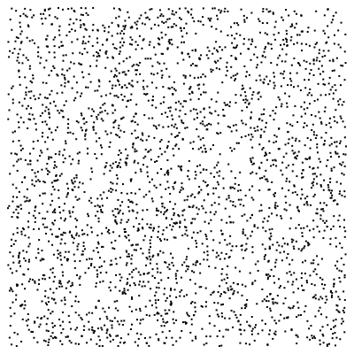
Now the way I have drawn Figure 7, it is a realization of a Poisson point process, i.e., a large number of independent uniformly distributed random points, whereas the joint distribution of many electrons with a wave function given by the wedge product of negative-energy eigenstates is not uniform in configuration space, as it vanishes at configurations with more than 4 particles at the same location; this fact should suppress clusters (i.e., many nearby particles), lead to an effective repulsion between the particles, and favor more evenly distributed configurations. So the correct picture should look more uniform than Figure 7.

Now the most uniform configuration conceivable would have exactly 2 particles at each location, as depicted in Figure 4 for a lattice. In the continuum limit, the appropriate figure for that, to compare with Figure 7, would seem to be a uniform shade of grey over all space, as depicted in Figure 8.

Thus, the correct picture should lie between Figures 7 and 8. If Conjecture 1 is correct, then we can say what the correct picture looks like: not at all like Figure 7 but like Figure 9.

That is, for a lattice with large $N$, the great majority of sites is occupied by 2 particles while only a number of sites much smaller than $N$ (one that remains finite in the limit $N\to\infty$) has occupation number different from 2. But in view of Figure 9, it seems natural to regard points with occupation number $\geq 3$ as electrons, those with $\leq 1$ as positrons, and those with $2$ as vacuum, i.e., to replace Figure 9 by Figure 10.

In sum, the “sea view” (that the Dirac sea should be taken literally) gets pushed by Conjecture 1 towards the ontology associated with $P_{\mathrm{nat}}$.

It is striking that the ontology suggested by Figure 7 breaks the symmetry between electrons and positrons: electrons are real and positrons are not. This symmetry is restored in the ontology associated with $P_{\mathrm{nat}}$. In fact, as Bjorken and Drell wrote [2, Sec. 5.2], we could have started equally well with the Dirac equation for the positrons (which amounts to using $\overline{\mathscr{H}_{1}}$ instead of $\mathscr{H}_{1}$) and would have arrived at the same theory. Here, of course, we go further than Bjorken and Drell and find the symmetry still respected in the position operators and, as we will see below, in the Bohmian trajectories.

In this section, I present reasons for thinking that with $P_{\mathrm{obv}}$, interaction locality (i.e., the absence of interaction terms between spacelike separated regions in the unitary time evolution) will not hold strictly but at most approximately. Some authors (e.g., Beck [1, Sec. 5.7]) have argued that interaction locality should not be expected to hold strictly. Likewise with propagation locality (i.e., the absence of faster-than-light propagation of wave functions):⁴⁴ 4 The Newton-Wigner position observable [30], which will not be considered here, is known [37] to violate propagation locality already in the 1-particle case. some authors (e.g., Soffer [36]) do not expect it to hold strictly. I tend to think that both hold strictly in our universe.

Be that as it may, here are two reasons for expecting $P_{\mathrm{obv}}$ to lead to conflicts with interaction locality.

The first reason concerns the question how a detector, if $P_{\mathrm{obv}}$ yields the detection probabilities, should collapse the wave function. Specifically, a function $f\in\mathscr{H}_{1+}$ that vanishes in an open set vanishes everywhere [37, Corollary 1.7], so $\rho_{\mathrm{obv}}$ can never have compact support. So consider a quantum state $\psi$ concentrated in the 1-electron, 0-positron sector according to $P_{\mathrm{obv}}$, suppose we apply a detector at $t=0$ and detect the particle in a compact region $A\subset\mathbb{R}^{3}$, say, a closed ball. Upon detection, the wave function should collapse. While it is not clear what exactly the post-collapse wave function $\psi^{\prime}$ should be, it is clear that the $(1,0)$-sector of $\psi^{\prime}$ will not be concentrated in $A$ but will have tails outside. In particular, there is positive probability of finding the particle far from $A$ at any $t>0$. Since with $P_{\mathrm{obv}}$ wave functions do not propagate faster than light (in fact, the Bohmian particle does not move faster than light), this leads to the conclusion that with positive probability, the particle actually was not in $A$ at $t=0$, so the detector in $A$ was triggered by a particle spacelike separated from $A$ in violation of interaction locality.

Here is the second reason: it seems that no conceivable interaction term would obey interaction locality with $P_{\mathrm{obv}}$ while conserving particle number, as illustrated by the following example. Assuming otherwise, consider a 2-electron wave function and let us write $\psi$ for the $(2,0)$-sector, $\psi=\psi^{20}_{s_{1}s_{2}}(\boldsymbol{x}_{1},\boldsymbol{x}_{2})$; consider $\psi$ at times $0$ and $t$. Let $F_{t}=\exp(-iH_{0}t)$ be the free time evolution. By interaction locality, $\psi_{t}$ agrees with $F_{t}\psi_{0}$ outside the $t$-neighborhood of the diagonal $\{(\boldsymbol{x}_{1},\boldsymbol{x}_{2}):\boldsymbol{x}_{1}=\boldsymbol{x}_{2}\}$ in configuration space $\mathbb{R}^{6}$. If both $\psi_{t}$ and $\psi_{0}$ lie in $\mathscr{H}_{1+}\otimes\mathscr{H}_{1+}$, then so does $\psi_{t}-F_{t}\psi_{0}$. But the only function in $\mathscr{H}_{1+}\otimes\mathscr{H}_{1+}$ that vanishes outside the $t$-neighborhood of the diagonal is 0. So, the evolution agrees with $F_{t}$, in contradiction to the assumption of interaction.

I close this section pointing out the widespread use of $P_{\mathrm{obv}}$. While it is standard in QFT to never mention a POVM, often remarks about how to interpret $\psi\in\mathscr{H}$ are inspired by $P_{\mathrm{obv}}$:

• •

  Thaller [37] p. 277: “the probability that there are just $n$ particles and [${\overline{n}}$] antiparticles at a given time is [$\|\psi^{n{\overline{n}}}\|^{2}$]”

• •

  Thaller [37] p. 277: “[$|\Omega\rangle$] describes the possibility that there are no particles at all”

• •

  Schweber [34] p. 230: “The basis vectors [$a^{\dagger}(P_{1+}x_{1})\cdots a^{\dagger}(P_{1+}x_{n})b^{\dagger}(P_{1-}{\overline{x}}_{1})\cdots$ $b^{\dagger}(P_{1-}{\overline{x}}_{\overline{n}})|\Omega\rangle$] span the states in which there exist [$n$] particles and [${\overline{n}}$] antiparticles.”

• •

  Schweber [34] p. 231: “[$\psi^{01}(x)$] is the probability amplitude for finding the antiparticle [at $\boldsymbol{x}$].”

None of these statements would be correct about $P_{\mathrm{nat}}$, all of them are correct about $P_{\mathrm{obv}}$.

I am not quoting these authors to criticize them. They made the statements I am quoting because they wanted to be clear and explicit about the physical meaning of certain quantum states; and for this they used $P_{\mathrm{obv}}$ or equivalent concepts, which is why I am quoting them.

References

- [1] C. Beck: Local Quantum Measurement and Relativity. Heidelberg: Springer (2021)
- [2] J.D. Bjorken and S.D. Drell: Relativistic Quantum Mechanics. McGraw-Hill (1964)
- [3] J.D. Bjorken and S.D. Drell: Relativistic Quantum Fields. McGraw-Hill (1965)
- [4] D. Bohm: Comments on an Article of Takabayasi concerning the Formulation of Quantum Mechanics with Classical Pictures. Progress in Theoretical Physics 9: 273–287 (1953)
- [5] D. Bohm and B.J. Hiley: The Undivided Universe: An Ontological Interpretation of Quantum Theory. London and New York: Routledge (1993)
- [6] H.J. Borchers: A remark on a theorem of B. Misra. Communications in Mathematical Physics 4: 315–323 (1967)
- [7] S. Colin, T. Durt, and R. Tumulka: On Superselection Rules in Bohm–Bell Theories. Journal of Physics A: Mathematical and General 39: 15403–15419 (2006) http://arxiv.org/abs/quant-ph/0509177
- [8] S. Colin and W. Struyve: A Dirac sea pilot-wave model for quantum field theory. Journal of Physics A: Mathematical and Theoretical 40: 7309–7342 (2007) http://arxiv.org/abs/quant-ph/0701085
- [9] D.-A. Deckert, D. Dürr, F. Merkl, and M. Schottenloher: Time Evolution of the External Field Problem in QED. Journal of Mathematical Physics 51: 122301 (2010) http://arxiv.org/abs/0906.0046
- [10] D.-A. Deckert, M. Esfeld, and A. Oldofredi: A persistent particle ontology for QFT in terms of the Dirac sea. British Journal for the Philosophy of Science 70(3): 747–770 (2019) http://arxiv.org/abs/1608.06141
- [11] D.-A. Deckert and F. Merkl: Dirac Equation with External Potential and Initial Data on Cauchy Surfaces. Journal of Mathematical Physics 55: 122305 (2014) http://arxiv.org/abs/1404.1401
- [12] D.-A. Deckert and F. Merkl: External Field QED on Cauchy Surfaces for Varying Electromagnetic Fields. Communications in Mathematical Physics 345: 973–1017 (2016) http://arxiv.org/abs/1505.06039
- [13] D.-A. Deckert and F. Merkl: A Perspective on External Field QED. Pages 381–399 in F. Finster, J. Kleiner, C. Röken, and J. Tolksdorf (editors), Quantum Mathematical Physics. Basel: Birkhäuser (2016) http://arxiv.org/abs/1510.03890
- [14] J. Dimock: Dirac Quantum Fields on a Manifold. Transactions AMS 269: 133–147 (1982)
- [15] J. Dimock: The Dirac Sea. Letters in Mathematical Physics 98: 157 (2011) http://arxiv.org/abs/1011.5865
- [16] D. Dürr, S. Goldstein, K. Münch-Berndl, and N. Zanghì: Hypersurface Bohm–Dirac Models. Physical Review A 60: 2729–2736 (1999) http://arxiv.org/abs/quant-ph/9801070
- [17] D. Dürr, S. Goldstein, R. Tumulka, and N. Zanghì: Bell-Type Quantum Field Theories. Journal of Physics A: Mathematical and General 38: R1–R43 (2005) http://arxiv.org/abs/quant-ph/0407116
- [18] D. Dürr and S. Teufel: Bohmian mechanics. Heidelberg: Springer (2009)
- [19] C.J. Fewster: A generally covariant measurement scheme for quantum field theory in curved spacetimes. Pages 253–268 in F. Finster, D. Giulini, J. Kleiner, and J. Tolksdorf (editors), Progress and Visions in Quantum Theory in View of Gravity, Berlin: Springer (2020) http://arxiv.org/abs/1904.06944
- [20] C.J. Fewster and R. Verch: Quantum fields and local measurements. Communications in Mathematical Physics 378: 851–889 (2020) http://arxiv.org/abs/1810.06512
- [21] S. Goldstein, T. Norsen, D.V. Tausk, and N. Zanghì: Bell’s Theorem. Scholarpedia 6(10): 8378 (2011) http://www.scholarpedia.org/article/Bell%27s_theorem
- [22] W. Greiner and J. Reinhardt: Quantum Electrodynamics, 4th ed. Heidelberg: Springer (2009)
- [23] R. Haag: Local quantum physics. Berlin: Springer (1992)
- [24] H. Halvorson and R. Clifton: No place for particles in relativistic quantum theories? Philosophy of Science 69: 1–28 (2002) http://arxiv.org/abs/quant-ph/0103041
- [25] G. Hegerfeldt: Remark on causality and particle localization. Physical Review D 10: 3320–3321 (1974)
- [26] G. Hegerfeldt and S.N.M. Ruijsenaars: Remarks on causality, localization, and spreading of wave packets. Physical Review D 22: 377 (1980)
- [27] M. Lienert and R. Tumulka: Born’s Rule for Arbitrary Cauchy Surfaces. Letters in Mathematical Physics 110: 753–804 (2020) http://arxiv.org/abs/1706.07074
- [28] S. Lill and R. Tumulka: Another Proof of Born’s Rule on Arbitrary Cauchy Surfaces. To appear in Annales Henri Poincaré (2021) http://arxiv.org/abs/2104.13861
- [29] D. Malament: In defense of dogma: Why there cannot be a relativistic quantum mechanics of (localizable) particles. Pages 1–10 in R. Clifton (editor): Perspectives on Quantum Reality: Non-Relativistic, Relativistic, and Field-Theoretic, Dordrecht: Kluwer (1996)
- [30] T.D. Newton and E.P. Wigner: Localized States for Elementary Systems. Reviews of Modern Physics 21(3): 400–406 (1949)
- [31] H. Reeh and S. Schlieder: Bemerkungen zur Unitäräquivalenz von Lorentz-invarianten Feldern. Il Nuovo Cimento 22: 1059–1068 (1961)
- [32] P. Pickl and D. Dürr: On Adiabatic Pair Creation. Communications in Mathematical Physics 282: 161 (2008) http://arxiv.org/abs/0704.2133
- [33] G. Scharf: Finite Quantum Electrodynamics, 2nd ed., Berlin: Springer (1995)
- [34] S. Schweber: An Introduction To Relativistic Quantum Field Theory. Row, Peterson and Company (1961)
- [35] D. Shale and W.F. Stinespring: Spinor representations of infinite orthogonal groups. Journal of Mathematics and Mechanics 14: 315–322 (1965)
- [36] A. Soffer: The Maximal Velocity of a Photon. Preprint (2011) http://arxiv.org/abs/1103.3031
- [37] B. Thaller: The Dirac Equation. Berlin: Springer (1992)
- [38] R. Tumulka: Positron Position Operators. II. A Simple Option. In preparation (2022)
- [39] J.C. Vink: Quantum mechanics in terms of discrete beables. Physical Review A 48: 1808–1818 (1993)