A Bayesian Model for Online Activity Sample Sizes
Thomas S. Richardson∗ Yu Liu∗ James McQueen Doug Hains
University of Washington Amazon.com Inc Amazon.com Inc Amazon.com Inc
Abstract
In many contexts it is useful to predict the number of individuals in some population who will initiate a particular activity during a given period. For example, the number of users who will install a software update, the number of customers who will use a new feature on a website or who will participate in an A/B test. In practical settings, there is heterogeneity amongst individuals with regard to the distribution of time until they will initiate. For these reasons it is inappropriate to assume that the number of new individuals observed on successive days will be identically distributed. Given observations on the number of unique users participating in an initial period, we present a simple but novel Bayesian method for predicting the number of additional individuals who will participate during a subsequent period. We illustrate the performance of the method in predicting sample size in online experimentation.
1 INTRODUCTION
There are many situations in which it is necessary to predict the number of individuals who will engage in an activity for the first time during some specified period. For example, a credit card company may want to predict the number of customers who respond to an offer for a new card; online e-commerce companies may want to predict the number of registered users who opt-in to new features or upgrade their membership. In the domain of online experimentation or A/B testing it is extremely useful to predict the number of individual users who will take part in the experiment as this can be used to estimate how long an experiment needs to run in order to get a sufficient sample size in order to achieve a desired power level. Such experiments are important as they provide a means by which “end-users can help guide the development of features” (Kohavi et al. 2007).
The problem that we consider in this paper is as follows: given a fixed population and observations on the number of unique individuals who initiate activity during an initial period of time, for example, a week, predict the number of additional individuals who will initiate activity during a subsequent period of time, for example one or three weeks.
Though formally the data can be seen as forming a time-series, the problem is not amenable to conventional time-series models. Though time-series model like ARIMA or Dynamic Regression have been used to predict the overall level of online traffic (Anderson 2016; Björklund and Hasselblad 2021), such models typically require long series and also assume stationarity of innovations after de-trending. Consequently, such methods are not suitable in many applications in which there is a wish to make predictions shortly after a new service has been launched. The data may also be viewed as a (non-stationary) counting process for which Hawkes processes are sometimes used (Hawkes 1971a; Hawkes 1971b). However, since the decision of each individual regarding when (or if) they will participate is taken independently, the process does not typically exhibit self-excitatory behavior of the type described by Hawkes processes.
Another challenge is that, in general, there will be heterogeneity within the population: some customers will initiate much more quickly than others; for example daily users of a mobile app will initiate much sooner than those who use it only for specific or occasional purposes. The users who are observed to initiate activity at the start of the observation period will be weighted more heavily towards frequent users than is the case subsequently. This unknown heterogeneity must be taken into account when making predictions for subsequent periods.
The primary contribution of this paper is the use of a hierarchical Bayesian Beta-Geometric model with censoring to model the heterogeneity of individuals in the population with respect to their propensity to initiate activity on any given day. Estimates for the number of additional individuals arriving in subsequent periods can then be obtained by simulating from the posterior predictive distribution. A convenient by-product of the simplicity of our model is that it is possible to sample from the posterior via straight Monte-Carlo simulation, thereby avoiding issues that may arise with Markov Chain approaches, such as assessing convergence and mixing times, which could present difficulties in large scale or fully-automated applications.
Relating the approach described here to prior work, there is a long history of using hierarchical beta-binomial models in Bayesian statistical inference for count data; see for example, Leonard 1972; Novick et al. 1973; Dempster et al. 1983. However, we are not aware of prior work that has applied these models to inference for the number of individuals initiating behavior in a given time period.
The rate at which customers participate in an online experiments, often called A/B tests, will have a great influence on the effect sizes that can be detected statistically within a given time period. Recent works outlining current best practice for such online experiments include Kohavi et al. 2007 and Bakshy et al. 2014. However, again to the best of our knowledge, previous work has not considered the specific question of predicting how many additional unique customers will be accrued in a subsequent time interval, given the number of unique customers who participated during an initial period. Such predictions are obviously of great relevance to decisions regarding the organization and scheduling of A/B experiments (Kohavi and Longbotham 2017; Casella and Berger 2021).
In section 2, we describe our proposed accrual model and the assumptions underlying it. In section 3, we describe how to make inferences about the number of additional individuals arriving in the second period by computing the posterior predictive distribution. In section 4 we illustrate the posterior distribution, predictive distributions and demonstrate the performance of our model on a large meta-analysis of A/B experiments.
2 ACCRUAL MODEL
Our goal here is to build a simple accrual model which uses the number of unique users or customers who first participate at day , to make a prediction regarding the total number of new (unique) customers who will participate in the second period of days. We take (first week) and a multiple of 7 (multiple weeks) in our data analyses.
2.1 Notations and Model Assumptions
Consider a set of customers indexed by and “Day ” means the -th day on which it was possible to participate.
Our model makes the simplifying assumption that each customer participates for the first time on any given day with a probability . We will also assume that if on day a customer has never participated previously, then their probability of participating on the next day remains . Consequently, the day of the experiment on which customer first participates will follow a Geometric distribution with probability .
2.2 Simple Accrual model: discrete
In the model that we propose below the underlying heterogeneity among customers in their behavior is described by modeling as being drawn from a distribution with support on . However, to provide intuition, before describing this model, consider first the simpler setting in which is discrete, taking different uniformly spaced values:
can be viewed as a characteristic of a customer. Thus it make sense to group together customers with the same value of . Let denote the number of customers in this group. Thus, in the simple setting described, there will be 100 groups of customers. It follows that the expected number of customers of type who first participate on Day will be , the expected number who first participate on Day will be , and the expected number participating on Day will be .
Consequently, in expectation, the set of customers who participate on Day 1 will consist of the following, ordered according to the value of :
Similarly, the set of customers who first participate on Day 2 will consist, in expectation, of the following:
Notice that relative to Day , a smaller proportion of people with participate for the first time on Day 2, since of such people already participated on Day . By repeating this procedure, we may simulate the number and type of customers who first participate on Day .
2.3 Accrual model: Geometric likelihood with censoring
We now consider a more realistic setting in which is continuous and build a model for the distribution of the participation probabilities . Similar to section 2.2, given the model assumptions, the day on which individual first participates will follow a Geometric distribution with probability :
| (1) |
For each individual who participates in the first period of length we will define to be the day on which they first participated; if an individual never participates in the first period, then we define . Thus , where, for example, if the first period, for which participation data is available, is a week. We formulate the model hierarchically, with a Beta distribution over the unknown participation probabilities. The model is specified formally as follows:
| (2) |
Note that the first term here can also be rewritten as:
Here indicates proportional to, while is the indicator function that takes the value if the condition is true and otherwise. follows a censored geometric distribution with success probability , where values larger than are censored and recorded as . We use the conjugate prior for , which is Beta. The hyper prior is a default prior recommended by Gelman et al. 2004[§5.3].
A graphical depiction of the proposed model is in Figure 1. is the individual-specific probability of customer participating on a given day. As described above, can be viewed as describing a given customer’s propensity to initiate activity. Similarly, the hyper-parameters , which determine the distribution from which the values are drawn, can be viewed as describing the character of different activities. For example, customers may be more likely to participate in an experiment changing the layout of the home page of a website than they might be to participate in an experiment changing the customer support contact page.
From the two assumptions given in Section 2.1, it follows that the parameters are i.i.d. conditional on the hyper parameters , . In other words, under the model each individual’s probability is an i.i.d. draw from a Beta distribution.
To understand and motivate the hyper prior, we first recall the following facts about Beta distributions:
If Beta then:
- (a)
.
- (b)
The variance is given by:
(3)
where we have used the fact that . Consequently, for large , , sd.
Consequently, the hyper-prior (2) corresponds to putting independent (improper) uniform priors on and . Note that the hyperprior (2) used here is improper; it does not integrate to . However, it will lead to a proper posterior provided that for at least one , ; see Gelman et al. 2004[Ex. 5.7].
3 INFERENCE FOR THE ACCRUAL MODEL
In this section, we discuss how to make predictions using the proposed accrual model.
3.1 Posterior predictive probability of continued non-participation
We first compute the elements in the formula of the posterior predictive distribution for future point in Figure 1. Let be the vector recording the day of the first participation or if there was no visit during the first period for individuals, and let be the individual-specific probabilities.
From Bayes rule, following the independence assumptions, we can obtain the joint posterior over parameters and hyper-parameters :
| (4) | ||||
Similarly we obtain the conditional posterior distribution over given hyper-parameters and the data :
|
|
(5) |
where we have used the fact that . Here (5) follows from the form of the joint posterior (4), which shows , where we use to indicate the ‘other’ elements of and likewise for ; the conditional independence here may also be obtained by applying the graphical d-separation criterion to the DAG shown in Figure 1. Thus from (5) we obtain:
|
|
(6) |
Similar to the development in Gelman et al. 2004[§5.3, Eq.(5.5) Eq.(5.8)], the posterior over the hyper-parameters , is then:
|
|
(7) |
For a given individual , who did not participate in the first period, so , we will define to be the first day on which the individual participates in the second period of length , or, as before, we define if they also never participate in the second period. Given the hyper-parameters , it follows from (5) that:
|
|
(8) |
Thus, conditional on hyper-parameters , the probability that an individual who has not participated in the first period will again not participate in the second period is:
| (9) | ||||
We express the probability of continued non-participation as a function of the full first period data because this determines the set of individuals who did not participate in the first period, for whom . Note that under the model this probability will be the same for all people who did not participate in the first week.
3.2 Predicting the number of new individuals in the second period
Let be the number of individuals who did not participate in the first period. Similarly, let be the subset of individuals who did not participate in the first period.
Given , the corresponding variables are i.i.d., and have probability of taking the value . It follows that given , the number of individuals who did not participate in the first period and who again did not participate in the second period will follow a binomial distribution, with the following parameters:11 1 Note that the posterior distribution for is not a Beta-Binomial distribution. is Binomial given , but the posterior over is not a Beta distribution.
| (10) |
Hence a simple Monte-Carlo scheme for simulating from the posterior for is as follows:
- 1.
Simulate , from the posterior distribution (7);
- 2.
For each value of draw a number from the Binomial distribution given by (10).
In step one we use the (straight) Monte-Carlo Ratio-of-Uniforms algorithm (Wakefield et al. 1991; Kinderman and Monahan 1977) to sample , . A point estimator of may be obtained by taking the median of the different draws from step 2. We use the posterior median as it is more robust than the posterior mean.
Thus the number of individuals who did not participate in the first period, but did participate in the second period is:
| no. of individuals participating | ||||
| for first time in Period 2 | (11) |
Hence we are able to efficiently obtain samples from the posterior for the number of additional individuals participating during the second period.
3.3 Inference when total population size is unknown
In the development so far, we have supposed that the number of censored observations, corresponding to individuals who did not show up in the first period, is known. This will hold in settings where the population of users is known, for example, where subscriptions or accounts are required for participation.. However, in some situations this may not be the case.
Fortunately, this turns out not to be a practical issue: provided that the number of censored observations is large relative to the number of uncensored observations, the posterior distribution for the number of additional individuals who will participate for the first time in the second period is not sensitive to the exact number of censored observations; see Section 4. In more detail, one may use a plug-in estimate of given by a multiple of the uncensored observations:
| (12) |
If necessary, can be tuned via cross-validation (James et al. 2013) on past data.
4 Experimental Results
In order to evaluate the performance of the model, we obtained participation data from experiments performed at Amazon.com, Inc. during the last year in the United States. We collected data from 1961 experiments that ran for at least 2 weeks, and 976 that ran for at least 4 weeks. For each experiment we used the number of new customers first participating in the experiment each day during the first week to predict the total sample size if the experiment were to continue running for weeks in total, where . (Axes in these plots are not annotated owing to business confidentiality.)
4.1 Illustrative Example
We first demonstrate the method using data from a single experiment that ran for at least 2 weeks. Figure 2(a) shows the participation data from the first week of the experiment. Here the X-axis represents the day index , while the Y-axis is the number of customers who first participate in the experiment on day .
Following the development in Section 3 for this experiment we first obtained samples from the joint posterior distribution over the hyper-parameters and , and then drew samples from the joint posterior predictive distribution for the number of new customers who first participate in each successive week. We define to be the number of new customers who first participate in the experiment on day . Thus the vector in Section 3.1 will consist of ones, twos …, sevens. Since data on the total population size was not available, the number of individuals who did not participate in the first week was estimated via (12) with ; note that this may be expressed as and is an estimate of the number of zeros in the vector . Here was selected by tuning from a set of four past experiments. Since can be large in some experiments, the use of the sufficient statistics ( can greatly speed up the computation relative to simply using .
For the experimental data shown in Figure 2(a), Figure 2(b) shows a scatterplot of 1000 samples of the hyper-parameters drawn from posterior distribution (7) together with an estimated density plot. We used an implementation of the (straight) Monte-Carlo Ratio-of-Uniforms algorithm (Wakefield et al. 1991; Kinderman and Monahan 1977; Northrop 2021; Northrop 2020) to obtain these samples. An implementation using sufficient statistics, based on code from the Bang package (Northrop 2020), can be found in github (Richardson and Liu 2022). The actual scales of the X and Y axes in Figure 2(b) are small indicating that, under the model, the posterior distribution for and is concentrated.
For each pair of values, we then use Equation (9) with to obtain samples from the joint posterior predictive distribution for the probability that an individual who did not participate in the experiment in the first week will again not participate in the subsequent 1, 2, 3 and 4 weeks if the experiment were to continue running. Plugging these probabilities and into Equation (10) results in predictions for the number of customers who did not participate in the initial period and who also do not participate in the second period of days, denoted where . Thus the predicted number of customers first participating in the experiment in the -th week is where and . We repeat this procedure for all pairs of and values. This results in samples from the posterior distribution over the function giving the number of new customers in each subsequent successive week. The 1000 predicted curves corresponding to the posterior draws are shown in Figure 2(c). The predicted curves show little variability, which is perhaps not surprising, given that the posterior over and , shown in Figure 2(b), is highly concentrated,
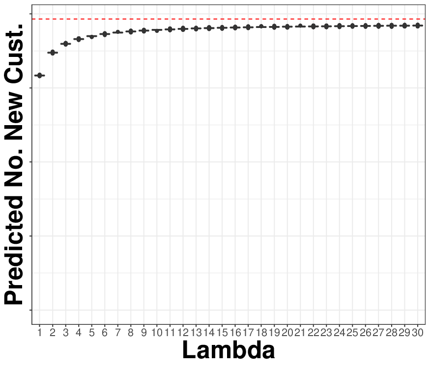
In Figure 3(a) we show how the predicted number of customers first participating in the experiment at week 2 is relatively insensitive to changes in . Specifically, Figure 3(a) shows boxplots giving 1000 posterior draws for each value of . As can be seen, when ranges from to , the median of the boxplot for the posterior predictive distribution is approximately constant. The red dotted line in this plot is the ground truth. Though the posterior median underestimates the ground truth, the accuracy is adequate for practical purposes.




4.2 Comparison of Bayesian Model to Other Approaches
We compared our approach to the following three baseline models: 1. Time-Series Models; 2. Log-Linear Models; 3. Random Forest Models. Results from two further baselines are given in the Supplementary Materials.
Time-series (ARIMA) models are widely used to predict online traffic trends (Anderson 2016; Björklund and Hasselblad 2021). However, there are several obstacles to applying such models in our context: (1) online A/B tests often take place during a relatively short experiment window and thus there are an insufficient number of observed time points; (2) The participation data are non-stationary requiring the specification of a model for the trend, but the trend here is of primary interest! (3) Though in some other settings it is possible to model the trend as a function of relevant baseline covariates, these may not be available. We fitted ARIMA models to the initial 7 days of data using auto.arima in the forecast R package (Hyndman et al. 2021). Random walk ARIMA(0, 1, 0) was fitted but generated very poor predictions. We also tried to de-trend using linear regression on the number of days , but this gives poor predictions due to the extrapolation. Since the time-series approaches were qualitatively much less competitive than the others, we do not consider these models further here.
Instead, we fitted a simple log-linear model:
| (13) |
where is the number of customers who first participate in the experiment on day and are independent errors with . Estimates for and may be obtained by linear regression of the log of the number of new participants on day against , for . The predicted number of new customers at week can be extrapolated by plugging in and then summing the predictions.
A Random Forest Model (Breiman 2001) is a flexible and general machine learning model. It uses bagging and ensemble techniques to obtain estimates from a set of regression trees. Here we assume that there is a training set of previous participation data, both from the initial period and the subsequent periods for a large set of experiments. In more detail, the -th row and -th column of the feature matrix is : the number of customers first participating in the experiment at day where . Let the response variable be , the number of customers first participating in the experiment at week , where . We fit 4 different random forest models on the training set: , where and make prediction for each model on the test set. We use the random forest package in R (Liaw and Wiener 2018) with 500 trees and default number of variables () randomly sampled as candidates at each split as parameters.
4.3 Predictive Performance
Figure 3(b) compares the predicted curves using the proposed Bayesian model, log linear regression, random forest regression and the ground truth for the example experiment in Figure 2(a). We use the median among 1000 simulations as the predictor for the proposed Bayesian model. For the random forest, the test data is the feature matrix of the target experiment while the training data are the feature matrix and responses for experiments (approximately 300) that took place before the target experiment. The selection of training data here mimics the way that such a model would be implemented in practice. As illustrated in Figure 3(b), the Bayesian predictor has the best performance in this illustrative example.
To assess performance on the full meta-analysis, we sort the 1961 experiments that ran for at least 2 weeks by their start date and, in order to accommodate the Random Forest, we split the first half of this set as the training dataset and the second half as the testing dataset. As before, we used in the Bayesian model. We repeat the same procedure for 976 experiments running for at least 4 weeks and predict the number of customers first participating at week 4. Figure 4 shows the true number of new customers participating in the experiment at the th week vs the predicted values using different methods. The line is shown in red in order to aid visual inspection of the performance of the various models. The plots suggest that (1) the Bayesian method has similar performance to the random forest model while the log linear predictor is unstable; (2) The Bayesian model tends to underestimate the ground truth.
We use the Root Mean Square Error (RMSE) and Mean absolute percentage error (MAPE) to quantify the predictive performance.
Table 1 compares the RMSE and MAPE for the random forest regression, log linear regression and the proposed Bayesian estimator. These results confirm that the Bayesian model slightly outperforms the log-linear and random forest model in terms of MAPE and has similar performance to the random forest model in terms of RMSE. Both models outperform the Log Linear model. Note that whereas the Random Forest model has access to training data, this is not used by the log-linear or Bayesian approaches (other than the four experiments that were used for selecting ).
| Week 2 | Week 4 | |||
| RMSE | MAPE | RMSE | MAPE | |
| Log-Lin | 1.84e+11 | 5.72e+5% | 9.06e+17 | 1.12e+13% |
| RF | 7.05e+05 | 44.06% | 5.49e+05 | 165.22% |
| Bayes | 7.11e+05 | 32.59% | 5.01e+05 | 84.57% |
In Appendix A we include additional experiments comparing the performance of the proposed method with a Neural Net model and a Censored Weibull model. These results confirm that the proposed method is competitive with the other methods.
Note that when is known the proposed Bayesian method does not require any past experiments as training data and thus may be applied in contexts where past experiments are either not available or have a different distribution compared to the target experiment; even when is unknown, only a small number of experiments are typically required to tune . In contrast, traditional machine learning methods, require training data from the same distribution. The latter assumption may not hold if experiments are conducted by different teams or at different times. Indeed, this may explain some of the results given in the Supplement, where the proposed Bayesian method outperforms the Random Forest in Table 2. Compared with the Log Linear and Censored Weibull methods, the proposed method is derived from a simple, interpretable model of customer behavior.
5 Conclusion
We have proposed a Bayesian approach to predict online activity in a fixed population. We demonstrated the utility of this method by applying it to predict sample size in online A/B testing. We evaluated the performance of our predictions by comparing them to the ground truth and other baselines in a large collection of online experiments. Our results show the practical utility of the proposed method.
The proposed Bayesian method does not require past experiments to use as training data when is known. It also does not require stationarity assumptions, or long observation periods. The proposed method also takes into consideration the heterogeneity within the population and thus captures differences in customer behavior when using online services. Our method is simple but effective, and is being used in production to predict sample sizes for online experiment in Amazon.
There are several further refinements that we intend to explore. As indicated by Figure 3(a), we found that in practice the proposed model typically slightly underestimates the ground truth. One possible explanation is that there may be growth in the pool of potential users that is occurring while the experiments is running. This suggests that it may be possible to improve predictions by incorporating additional (dynamic) information regarding population size.
References
- Anderson (2016) Linda Anderson. Library website visits and enrollment trends. Evidence Based Library and Information Practice, 11(1):4, 2016.
- Bakshy et al. (2014) Eytan Bakshy, Dean Eckles, and Michael S. Bernstein. Designing and deploying online field experiments. In Proceedings of the 23rd International Conference on the World Wide Web, pages 283–292, 2014.
- Björklund and Hasselblad (2021) Martin Björklund and Felix Hasselblad. The effect of online advertising in a digital world: Predicting website visits with dynamic regression, 2021.
- Breiman (2001) Leo Breiman. Random forests. Machine learning, 45(1):5–32, 2001.
- Casella and Berger (2021) George Casella and Roger L. Berger. Statistical inference. Cengage Learning, 2021.
- Dempster et al. (1983) Arthur P. Dempster, Murray R. Selwyn, and Barbara J. Weeks. Combining historical and randomized controls for assessing trends in proportions. Journal of the American Statistical Association, 78(382):221–227, 1983.
- Gelman et al. (2004) Andrew Gelman, John B. Carlin, Hal S. Stern, and Donald B. Rubin. Bayesian Data Analysis. Chapman and Hall/CRC, 2nd edition, 2004.
- Hawkes (1971a) Alan G. Hawkes. Spectra of some self-exciting and mutually exciting point processes. Biometrika, 58(1):83–90, 04 1971a.
- Hawkes (1971b) Alan G. Hawkes. Point spectra of some mutually exciting point processes. Journal of the Royal Statistical Society. Series B (Methodological), 33(3):438–443, 1971b.
- Hyndman et al. (2021) Rob Hyndman, George Athanasopoulos, Christoph Bergmeir, Gabriel Caceres, Leanne Chhay, Mitchell O’Hara-Wild, Fotios Petropoulos, Slava Razbash, Earo Wang, and Farah Yasmeen. forecast: Forecasting functions for time series and linear models, 2021. URL https://cran.r-project.org/web/packages/forecast/forecast.pdf. R package version 8.15.
- James et al. (2013) Gareth James, Daniela Witten, Trevor Hastie, and Robert Tibshirani. An Introduction to Statistical Learning, volume 112. Springer, 2013.
- Kay (1977) Richard Kay. Proportional hazard regression models and the analysis of censored survival data. Journal of the Royal Statistical Society: Series C (Applied Statistics), 26(3):227–237, 1977.
- Kinderman and Monahan (1977) Albert J. Kinderman and John F. Monahan. Computer generation of random variables using the ratio of uniform deviates. ACM Transactions on Mathematical Software (TOMS), 3(3):257–260, 1977.
- Kohavi and Longbotham (2017) Ron Kohavi and Roger Longbotham. Online controlled experiments and A/B testing. Encyclopedia of machine learning and data mining, 7(8):922–929, 2017.
- Kohavi et al. (2007) Ron Kohavi, Randal M. Henne, and Dan Sommerfield. Practical guide to controlled experiments on the web: listen to your customers not to the hippo. In Proceedings of the 13th ACM SIGKDD International Conference on Knowledge Discovery and Data Mining, pages 959–967, 2007.
- Leonard (1972) Thomas Leonard. Bayesian methods for binomial data. Biometrika, 59:581–589, 1972.
- Liaw and Wiener (2018) Andy Liaw and Matthew Wiener. R package random Forest, 2018. URL https://cran.r-project.org/web/packages/randomForest/randomForest.pdf. R package version 4.6-14.
- Liu et al. (2021) C. H. Bryan Liu, Ângelo Cardoso, Paul Couturier, and Emma J McCoy. Datasets for online controlled experiments. Proceedings of the Neural Information Processing Systems Track on Datasets and Benchmarks, 2021; arXiv:2111.10198, 2021.
- Northrop (2020) Paul J. Northrop. R package bang: Bayesian Analysis, No Gibbs, 2020. URL https://cran.r-project.org/web/packages/bang/index.html. R package version 1.0.1.
- Northrop (2021) Paul J. Northrop. R package rust: Ratio-of-Uniforms Simulation with Transformation, 2021. URL https://cran.r-project.org/web/packages/rust/index.html. R package version 1.3.12.
- Novick et al. (1973) Melvin R. Novick, Charles Lewis, and Paul H. Jackson. The estimation of proportions in groups. Psychometrika, 38(1):19–46, 1973.
- Paszke et al. (2019) Adam Paszke, Sam Gross, Francisco Massa, Adam Lerer, James Bradbury, Gregory Chanan, Trevor Killeen, Zeming Lin, Natalia Gimelshein, Luca Antiga, Alban Desmaison, Andreas Kopf, Edward Yang, Zachary DeVito, Martin Raison, Alykhan Tejani, Sasank Chilamkurthy, Benoit Steiner, Lu Fang, Junjie Bai, and Soumith Chintala. PyTorch: An imperative style, high-performance deep learning library. In Advances in Neural Information Processing Systems, volume 32, pages 8024–8035, 2019.
- Richardson and Liu (2022) Thomas S. Richardson and Yu Liu. Hierarchical Bayesian Analysis with Bang, 2022. URL https://github.com/amazon-research/hierarchical-bayesian-analysis-with-bang.
- Wakefield et al. (1991) Jonathan C. Wakefield, Alan E. Gelfand, and Adrian F. M. Smith. Efficient generation of random variates via the ratio-of-uniforms method. Statistics and Computing, 1(2):129–133, 1991.
Supplementary Material:
A Bayesian Model for Online Activity Sample Sizes
Appendix A ADDITIONAL EXPERIMENTS
Prompted by a suggestion from the reviewers, we added two additional baseline models for comparison, a Neural Network model and a Censored Weibull model. In addition, we compared the performance of all these methods on a recent public dataset containing online experiments (Liu et al. 2021); among the 78 experiments in this set, 10 (respectively, 8) experiments contain complete daily sample sizes from day to (respectively, 28). We show the results of predictions on these experiments in Table 2; given the small size of this public dataset, the Random Forest and Neural Net models were trained on the proprietary data.
In more detail, the Censored Weibull model (Kay 1977) was fitted via maximum likelihood with data from week 1 (plus estimated by (12)). The Neural Network (Paszke et al. 2019) used Relu as activation function and 3 hidden layers with 16, 32 and 16 nodes respectively; training data was used as a validation dataset to tune other parameters.
The results from Table 2 confirm that the proposed Bayesian model is competitive against all the other methods considered. We also note here that the Neural Net method requires greater computational resources than the other methods considered and hence is less scalable.
Lastly, following another suggestion from the reviewers, in the last two rows of the Table we compare results for the posterior mean and median of the Bayesian method. In our experiment they are statistically indistinguishable.
| Method | Public Data | Proprietary data used in paper (additional | ||||||
| results for NN and Weibull) | ||||||||
| Week 2 | Week 4 | Week 2 | Week 4 | |||||
| RMSE | MAPE | RMSE | MAPE | RMSE | MAPE | RMSE | MAPE | |
| RF + | 6.48e+5 | 22.78% | 1.79e+6 | 50.43% | 7.05e+05 | 44.06% | 5.49e+05 | 165.22% |
| training data | ||||||||
| NN + | 1.10e+6 | 47.58% | 1.92e+6 | 115.86% | 5.64e+05 | 4.65e+3% | 5.81e+05 | 490.41% |
| training data | ||||||||
| Log-linear | 1.12e+5 | 19.06% | 6.86e+5 | 67.93% | 1.84e+11 | 5.72e+5% | 9.06e+17 | 1.12e+13% |
| Censored | 4.36e+5 | 32.42% | 3.09e+5 | 70.97% | 1.85e+06 | 49.17% | 1.41e+06 | 139.68% |
| Weibull | ||||||||
| Bayesian | 1.59e+5 | 12.79% | 5.09e+5 | 15.24% | 7.11e+05 | 32.57% | 5.01e+05 | 84.55% |
| (mean) | ||||||||
| Bayesian | 1.59e+5 | 12.78% | 5.09e+5 | 15.25% | 7.11e+05 | 32.59% | 5.01e+05 | 84.57% |
| (median) | ||||||||