^†^†footnotetext: These authors contributed equally to this work.
Emails: lostaglio@protonmail.com, korzekwa.kamil@gmail.com

Continuous thermomajorization and a complete set of laws
for Markovian thermal processes

Matteo Lostaglio^∗, Affiliation: Korteweg-de Vries Institute for Mathematics and QuSoft, University of Amsterdam, The Netherlands Affiliation: QuTech, Delft University of Technology, P.O. Box 5046, 2600 GA Delft, The Netherlands Kamil Korzekwa^∗, Affiliation: Faculty of Physics, Astronomy and Applied Computer Science, Jagiellonian University, 30-348 Kraków, Poland

Abstract

The standard dynamical approach to quantum thermodynamics is based on Markovian master equations describing the thermalization of a system weakly coupled to a large environment, and on tools such as entropy production relations. Here we develop a new framework overcoming the limitations that the current dynamical and information theory approaches encounter when applied to this setting. More precisely, we introduce the notion of continuous thermomajorization, and employ it to obtain necessary and sufficient conditions for the existence of a Markovian thermal process transforming between given initial and final energy distributions of the system. These lead to a complete set of generalized entropy production inequalities including the standard one as a special case. Importantly, these conditions can be reduced to a finitely verifiable set of constraints governing non-equilibrium transformations under master equations. What is more, the framework is also constructive, i.e., it returns explicit protocols realizing any allowed transformation. These protocols use as building blocks elementary thermalizations, which we prove to be universal controls. Finally, we also present an algorithm constructing the full set of energy distributions achievable from a given initial state via Markovian thermal processes and provide a Mathematica implementation solving $d=6$ on a laptop computer in minutes.

I Introduction

It is well-known that thermodynamics can be formulated in the resource theory language of information theory Lostaglio 2019; Janzing et al. 2000; Horodecki and Oppenheim 2013; Brandão et al. 2015; Ng and Woods 2018; Vinjanampathy and Anders 2016. Since it focuses only on input-output relations under a class of quantum operations, the resource theory is unable to discuss how the process is realized in time, nor does it involve the notions of entropy production or master equations, even though the latter are commonplace in standard approaches. As such, the standard and the resource-theoretic frameworks are for the most part disconnected. Somewhat surprisingly, despite all its powerful theorems, the resource theory has not affected the analysis of a thermodynamics practitioner following the more explicit dynamical approaches based on the master equation formalism Kosloff 2013.

The aim of this work is to overcome this situation by showing how to unify the master equations and information theory tools. We first summarize the basic notions of both approaches to thermodynamics in Sec. II, and demonstrate the insufficiency of each of them, when taken separately, to capture relevant thermodynamic constraints. Then, in Sec. III, we propose a hybrid approach that can overcome these limitations. In constructing our solution we highlight the necessity of finding a finitely verifiable set of thermodynamic laws specifying when one state can be thermodynamically transformed into another one. Furthermore, we wish to go beyond the question of whether a thermodynamic transformation exists, and ask how it should be realized. The resource theory approaches are for the most part silent about the latter, which is arguably a central obstacle to their application to concrete problems. Our framework, on the contrary, will be constructive.

In Sec. IV we introduce our main novel technical tool, continuous thermomajorization, which extends the concept of thermomajorization introduced in Refs. Ruch et al. 1978; Horodecki and Oppenheim 2013. We prove that this partial order of energy distributions provides necessary and sufficient conditions for the existence of a thermalization process generated by a Markovian master equation. More precisely, we show that an out of equilibrium energy distribution can be transformed into another one by a Markovian thermal process if and only if the former continuously thermomajorizes the latter. We then connect with the notion of entropy production Landi and Paternostro 2021 in Sec. V, where we show that continuous thermomajorization allows one to identify a complete set of generalized entropy production relations, including the standard one as a special case.

Our ultimate goal, however, is to find a finitely-verifiable set of such conditions. To achieve this, we first prove in Sec. VI that elementary thermalizations, generated by simple reset master equations on two-level submanifolds, form universal controls in the Markovian regime. In other words, every state transformation that can be achieved by a Markovian thermal process can also be achieved by a sequence of elementary thermalizations. Employing this simplified set of controls, in Sec. VII we show that continuous thermomajorization indeed can be checked in a finite number of steps. Remarkably, we can also return the exact sequence of elementary controls required to realize any allowed transformation. As a final result of our paper, in Sec. VIII we provide an explicit algorithm verifying the continuous thermomajorization relation between any two vectors, and offer a Mathematica implementation Korzekwa 2021 that checks the conditions for systems of dimension up to $7$ in a matter of hours on a standard laptop computer.

While this work focuses on developing the technical machinery, in the accompanying paper Korzekwa and Lostaglio 2022 we illustrate how one can employ it to design provably optimal thermodynamic protocols. There, we apply our results to study the effects of memory on work fluctuations, to explicitly construct optimal cooling protocols, and to showcase the important role played by catalysts in practical scenarios. We also report on a recent work which used our results to show that non-Markovianity boosts the efficiency of thermal bio-molecular switches Spaventa et al. 2022. All these build up encouraging evidence that the framework is suitable both for providing model-independent bounds, as well as for algorithmically constructing new thermodynamics protocols when a complete analysis is unattainable by either analytic or numerical methods.

II Setting the scene

II.1 Thermodynamic frameworks

II.1.1 The traditional approach

A general open dynamics of a $d$ -dimensional quantum system is described by a quantum channel, i.e., a completely positive trace-preserving map acting on the quantum state $\rho$ Nielsen and Chuang 2010. However, in a thermodynamic setting, we are often interested in the evolution of such a quantum system interacting with a large thermal bath at inverse temperature $\beta=1/(k_{B}T)$ , where $k_{B}$ is Boltzmann constant and $T$ is the temperature of the bath. Typical microscopic derivations employing the weak coupling limit Breuer and Petruccione 2002; Kosloff 2013; Alicki and Kosloff 2018 then lead to a master equation with the general form Gorini et al. 1976; Lindblad 1976:

\frac{d\rho(t)}{dt}={\cal H}(\rho(t))+\mathcal{L}_{t}(\rho(t)).

(1)

The first term, ${\cal H}$ , is the generator of a closed (reversible) quantum dynamics,

{\cal H}(\rho)=-i[H,\rho],

(2)

with $[\cdot,\cdot]$ denoting the commutator, $[A,B]=AB-BA$ , and $H$ being the (dressed) Hamiltonian of the system, which we assume to be time-independent. The second term, $\mathcal{L}_{t}$ , is known as the Lindbladian or dissipator and generates an open (irreversible) quantum dynamics. It has the following general form

\!\!\!\mathcal{L}_{t}(\rho)=\sum_{i}r_{i}(t)\left(\!L_{i}(t)\rho L_{i}(t)^{\dagger}-\frac{1}{2}\{L_{i}(t)^{\dagger}L_{i}(t),\rho\}\!\right)\!,\!

(3)

with $\{\cdot,\cdot\}$ denoting the anticommutator, $\{A,B\}=AB+BA$ , $L_{i}(t)$ being time-dependent jump operators, and $r_{i}(t)$ being time-dependent non-negative jump rates.

While a general Lindbladian only requires the rates $r_{i}$ to be non-negative, Lindbladians arising from the interaction of a quantum system with a large heat bath have two standard properties Breuer and Petruccione 2002; Kosloff 2013; Alicki and Kosloff 2018:

(P1)

Stationary thermal state. The Gibbs thermal state of the system,

$\gamma=\frac{e^{-\beta H}}{\mathrm{Tr}\left(e^{-\beta H}\right)},$ (4)

is a stationary solution of the dynamics, i.e.,

$\forall t:\quad\mathcal{L}_{t}\gamma=0.$ (5)
(P2)

Covariance. The Lindbladian ${\cal L}_{t}$ commutes with the generator of the Hamiltonian dynamics ${\cal H}$ at all times $t$ , i.e.,

$\forall\rho:\quad\mathcal{L}_{t}(\mathcal{H}(\rho))=\mathcal{H}(\mathcal{L}_{t}(\rho)).$ (6)

For brevity, we will refer to the quantum dynamics generated by master equations in the form of Eq. (1) and satisfying properties (P1)-(P2) as Markovian thermal processes:

Definition 1.

A channel $\mathcal{T}$ is a Markovian thermal process (MTP) if it results from integrating a Markovian master equation, Eq. (1), between time $0$ and $t_{f}\in[0,+\infty]$ , where the Lindbladian $\mathcal{L}_{t}$ satisfies properties (P1)-(P2).

These form a standard description of thermalization in the field of quantum thermodynamics and beyond (see, e.g., Sec. 3.1 of Ref. Alicki and Kosloff 2018), and will be the main focus of this work. The most well-known and important constraint on the allowed thermodynamic transitions under MTP takes the form of a sort of $H$ -theorem Alicki and Kosloff 2018:

\displaystyle\frac{d\Sigma(t)}{dt}:=

\displaystyle-\frac{d}{dt}S(\rho(t)\|\gamma)\geq 0,

(7)

where

S(\rho\|\gamma)=\mathrm{Tr}\left(\rho(\log\rho-\log\gamma)\right)

(8)

is the quantum relative entropy and $d\Sigma/dt$ is known as the entropy production (relative to $\gamma$ ) Spohn 1978. One can recognize in this equation the standard second law of thermodynamics:

\frac{d\Sigma(t)}{dt}=\frac{dS(t)}{dt}-\beta J(t)\geq 0,

(9)

with


$\displaystyle S(t)$	$\displaystyle:=-\mathrm{Tr}\left(\rho(t)\log\rho(t)\right),$	(10a)
$\displaystyle J$	$\displaystyle:=\mathrm{Tr}\left(H\frac{d\rho(t)}{dt}\right),$	(10b)

being the von Neumann entropy and the heat current flowing to the system, respectively.

A typical example of a Markovian thermal process is the quantum optical master equation Breuer and Petruccione 2002, which describes the evolution of a two-dimensional quantum system with $H=\frac{\hbar\omega}{2}(\left|1\right\rangle\!\!\left\langle 1\right|-\left|0\right\rangle\!\!\left\langle 0\right|)$ interacting weakly with a thermal radiation field. The quantum optical master equation is of the form given in Eq. (1), with the jump operators and the corresponding rates given by


$\displaystyle L_{1}$	$\displaystyle=\left\|0\right\rangle\!\!\left\langle 1\right\|,\quad r_{1}(t)=r(N+1),$	(11a)
$\displaystyle L_{2}$	$\displaystyle=\left\|1\right\rangle\!\!\left\langle 0\right\|,\quad r_{2}(t)=rN,$	(11b)

where $N$ is the average number of photons at the resonant frequency $\omega$ and $r$ is the spontaneous emission rate.

While it is not straightforward to characterize all physical setups modelled via MTPs, they are commonplace. A crucial observation to be kept in mind is the following: MTPs constitute an effective model that emerges after common approximations (such as the secular approximation, ignoring the Lamb shift) and in an appropriate frame (in general, a rotating frame). For a concrete example of such an emergence after relevant approximations, consider a typical setup of discrete quantum heat engines in the weak coupling regime. There, one assumes that the dissipators only operate for a given amount of time, and they are then suddenly switched to new ones according to some schedule. This is a special case of Eq. (3) where $L_{i}(t)\equiv L_{i}$ , $r_{i}(t)$ are taken to be appropriate step functions and $H$ is (approximatively) constant after ignoring a small Lamb shift.¹¹ 1 Just to make an example among many, Ref. Uzdin et al. 2015 involves this kind of “implicit” time dependence on the dissipators only (after rotating wave approximation). Often these dissipators are associated to baths at different temperatures coupled to different energy submanifolds, but nothing prevents us to consider the special case where the baths are at the same temperature. These are not only a nice class of examples: as we show in Theorem 3, these controls are sufficient to realize every transformation that can be achieved by a generic MTP.

Thus, any model that can be formally written as Eq. (1) with properties (P1)-(P2) (with or without time-dependence on $\mathcal{L}_{t}$ ) falls within the scope of this work. These include incoherent noise in quantum computers Campbell et al. 2017 and effective models describing fluorescence and other non-radiative decay channels in atoms, molecules and nanostructures. The formal equivalence between thermodynamic and other models of dissipation is well-known and it is in fact leveraged as a standard technique to realize effective heat baths Klatzow et al. 2019. In quantum information terms, depolarization and amplitude damping can be seen as limiting cases of Markovian thermal processes when $\beta\rightarrow 0$ and $\beta\rightarrow\infty$ , respectively. This means that, in principle, our results apply well-beyond the obvious thermodynamic scenarios. Here, we study Markovian thermal processes independently of what application one has in mind. In the accompanying paper Korzekwa and Lostaglio 2022, we present examples of how the formalism can be applied in practice.

Having said that, there are of course several relevant scenarios that fall beyond the scope of MTPs. We will discuss the potential and need for further generalizations of the MTP framework after discussing the resource-theory approach.

II.1.2 The resource-theoretic approach

The notion of a Markovian thermal process should be contrasted with the notion of a thermal operation Horodecki and Oppenheim 2013 or the closely related notion of a thermal process Gour et al. 2018, used in the resource theory of quantum thermodynamics:

Definition 2.

Thermal processes (TP) are all channels $\mathcal{E}$ that satisfy the two conditions analogous to (P1)-(P2):


$\displaystyle\mathcal{E}(\gamma)$	$\displaystyle=\gamma,$	(12a)
$\displaystyle\forall\rho,t:\quad\mathcal{E}(e^{-iHt}\rho e^{iHt})$	$\displaystyle=e^{-iHt}\mathcal{E}(\rho)e^{iHt},$	(12b)

with $\gamma$ defined in Eq. (4).

Examples of thermal processes include all thermal operations, i.e. dynamics induced by generic energy-preserving unitary interactions between the system and an environment $E$ described by an arbitrary Hamiltonian $H_{E}$ and prepared in a thermal Gibbs state $\gamma_{E}$ at fixed inverse temperature $\beta$ Brandão et al. 2013; Brandão et al. 2015; Lostaglio 2019. When such a transformation exists between the initial and final states, $\rho(0)$ and $\rho(t_{f})$ , we will write

\rho(0)\stackrel{{\scriptstyle\textrm{TP}}}{{\longmapsto}}\rho(t_{f}).

(13)

The resource theory is concerned with giving necessary and sufficient conditions for Eq. (13). Because of the symmetries inherent in the thermodynamic processes under consideration, it is convenient to represent the state of the system $\rho(t)$ at time $t$ by a vector $\bm{p}(t)$ of populations (energy distributions) and a matrix $C(t)$ of coherences, defined as


$\displaystyle p_{i}(t)$	$\displaystyle=\langle{E_{i}}\|\rho(t)\|{E_{i}}\rangle,$	(14a)
$\displaystyle C_{ij}(t)$	$\displaystyle=\langle{E_{i}}\|\rho(t)\|{E_{j}}\rangle\quad\mathrm{for~}i\neq j,$	(14b)

where $|{E_{i}}\rangle$ is the eigenstate of $H$ corresponding to energy $E_{i}$ (for simplicity we consider non-degenerate $H$ ). When $\rho(0)$ and $\rho(t_{f})$ are diagonal (i.e., $C(0)=C(t_{f})=0$ ), the conditions for Eq. (13) are the well-known thermomajorization constraints of Ref. Horodecki and Oppenheim 2013.²² 2 In fact, the case $C(0)=0$ , $C(t_{f})\neq 0$ is trivial, since these transformations are always forbidden. The problem for general states was formally solved by the remarkable work in Ref. Gour et al. 2018, where an extremely complex but complete set of entropy conditions was derived.

One can readily see, e.g. by taking a thermal operation with $E$ being a small environment, that the resource theory and the standard framework apply to different regimes. For a concrete and relevant example, consider a single qubit system and take the environment defining the thermal operation to be given by a single bosonic oscillator in resonance with it. Take the energy-preserving unitary interaction $U(t)=\exp(-itH_{\rm int})$ with the interaction Hamiltonian from the Jaynes-Cummings model:

H_{\rm int}=g(\left|1\right\rangle\!\!\left\langle 0\right|\otimes a+\left|0\right\rangle\!\!\left\langle 1\right|\otimes a^{\dagger}),

(15)

with $a^{\dagger}$ and $a$ denoting the bosonic creation and annihilation operators, and $g$ being a coupling constant. No Markovian master equation like Eq. (1) can be derived. In fact, the dynamics is fully solvable, so one can compute $\rho(t)$ and verify that the entropy production relation from Eq. (7) is violated due to non-Markovian effects. The resource theory approach, in allowing fine control over memory effects and system-bath correlations, does not incorporate the Markovianity condition of standard thermalization processes.

II.1.3 Potential and need for generalizations of the MTP model

The scenarios that fall beyond the scope of MTPs are most prominently those involving an explicit time-dependence. Even then, however, our framework can still be useful, e.g., $4$ -stroke engines have separate thermalization and unitary strokes, and our framework can be used to study the former steps (see the accompanying paper Korzekwa and Lostaglio 2022 where this strategy is explicitly used to study a cooling problem). Importantly, such engines with separate thermalization and unitary steps are thermodynamically universal in the weak coupling regime Uzdin et al. 2015. Thus, in this regime, our framework allows one to explore the full potential of quantum heat engines.

However, if one wants to explicitly study thermalization dynamics with an external driving field, then using the MTP model may become problematic. Suppose that one simply allows in Eq. (1) an arbitrary time-dependence in $H$ , even adding the extra constraint that zero net work is done to the system in (almost) any run. Then, the results of Ref. Perry et al. 2018 imply that these extended controls simulate arbitrary energy-preserving interactions with a thermal environment of any dimensionality, including generic non-Markovian effects (see also Refs. Vom Ende et al. 2019; Schulte-Herbrüggen et al. 2020 for related results). In other words, extending the controls in this way, we recover the standard resource-theoretic approach based on thermal processes discussed above, which does not include the relevant constraints of the Markovian master equation approach to thermodynamics.

Hence, one needs to be very careful in how time-dependence is introduced in the framework. If we are striving to relate the resource theory framework to the standard theory of open quantum systems via Markovian master equations, as we are doing here, we need a more restricted setting. We leave open the question of how to formally generalize MTP further (say, introducing slow driving) without dropping the core Markovianity constraint that we want to impose on the dynamics. The dialogue between resource theories and open quantum system dynamics initiated by this work is far from over.

II.2 Insufficiency of current approaches

Quantum thermodynamics aims at deriving laws holding independently of the particular dynamics. In other words, based on minimal assumptions (such as assuming that the environment the system interacts with is thermal), one wants to constrain possible state transformations of the system. In what follows we discuss how both the resource-theoretic and the standard approaches fare in this regard, and highlight some important limitations that we wish to overcome with the present contribution. We will consider the stereotypical situation of a system put into a weak thermal contact with a thermal bath at inverse temperature $\beta$ . The crucial question is: given a quantum system initially described by a known energy distribution $\bm{p}(0)$ , what general conditions determine the possible $\bm{p}(t)$ achievable at some later time $t$ ?

II.2.1 Insufficiency of the traditional approach

The second law in the form of Eq. (7) provides a set of conditions that can help us answer the question posed. In fact, the second law provides a functional on the set of states that must be monotonically non-decreasing along the dynamics. To explain its usefulness and limitations, let us focus on a simple example of an incoherent three-level system, i.e., with $d=3$ and $C(0)=0$ . Due to the covariance of Markovian thermal processes (property (P2)), we necessarily have $C(t)=0$ for all $t>0$ .³³ 3 This is because $C(0)=0$ is equivalent to $\mathcal{H}(\rho(0))=0$ , and (P2) then implies $\mathcal{H}(\mathcal{L}_{t}(\rho(0)))=0$ . Thus, the state at time $\delta t$ is stationary, $C(\delta t)=0$ , and the argument extends to all $t>0$ . Thus, the entropy $\Sigma$ reads

\Sigma(t)=-\sum_{i=1}^{3}p_{i}(t)(\log p_{i}(t)-\log\gamma_{i}),

(16)

where $\bm{\gamma}$ denotes the vector of thermal populations. We plot the values of $\Sigma$ in the simplex of all 3-dimensional probability distributions in Fig. 1a, for one particular choice of $\bm{\gamma}$ . Then, we can verify whether there exists a continuous path $\bm{p}(t)$ connecting a given initial $\bm{p}(0)$ with the final $\bm{p}(t_{f})$ , with constantly non-decreasing $\Sigma(t)$ along the path (as required by the second law). In particular, for two states with equal entropy $\Sigma$ there is a unique isoentropic path connecting them, and the second law in the form of positive entropy production does not forbid such a transition.

Figure 1: Thermodynamic entropy landscape for a three-level incoherent system. The state of an incoherent system is represented by a vector of populations

\bm{p}=(p_{1},p_{2},1-p_{1}-p_{2})

, and the chosen thermal state is

\bm{\gamma}=(0.7,0.2,0.1)

. (a) Entropy functional

\Sigma

. The black dashed trajectory is the path of constant

\Sigma

. The constraint of positive entropy production cannot exclude that the thermodynamic transition from

\bm{p}(0)

\bm{p}(t)

is allowed. (b) Entropy functional

\Sigma_{2}

. The black dashed trajectory is the path of constant

\Sigma

. The constraint of positive collisional entropy production implies that one cannot transform

\bm{p}(0)

into

\bm{p}(t)

However, one can prove that for most pairs of isoentropic states there is no Markovian thermal process that can map between them, independently of the chosen controls and details of the environment. What the standard second law is missing is that there exist generalized (non-equilibrium) entropy production relations that must be satisfied for a thermodynamic transformation to be allowed. As we will discuss later in Sec. V, one of them is the non-negativity of the collisional entropy production (with respect to $\bm{\gamma}$ ):

\frac{d\Sigma_{2}(t)}{dt}:=-\frac{d}{dt}S_{2}(\bm{p}(t)\|\bm{\gamma})\geq 0,

(17)

where

S_{2}(\bm{p}\|\bm{\gamma}):=\log\left(\sum_{i=1}^{d}\frac{p_{i}^{2}}{\gamma_{i}}\right),

(18)

is the relative Rényi entropy of order two Renyi 1961. Eq. (17) provides an independent monotonically non-decreasing functional for the thermodynamic system. As before, we plot the values of $\Sigma_{2}$ in Fig. 1b for the same choice of $\bm{\gamma}$ , so that we can clearly see that the path which kept $\Sigma$ constant is decreasing $\Sigma_{2}$ . Decreasing the collisional entropy (relative to $\bm{\gamma}$ ) is forbidden, hence the transition is impossible under any Markovian thermal process. This rules out, by means of an explicit counterexample, that the standard entropy production functionals (often referred to as the second law of thermodynamics in the literature) faithfully characterizes thermalization out of equilibrium.

II.2.2 Insufficiency of the resource-theoretic approach

If the standard entropy production constraint is insufficient, the information theory-minded reader could wonder whether the results of the resource theory approach can come to the rescue. Here we will argue why these tools, in their present form at least, are too weak to capture the relevant limitations of quantum thermodynamics in the Markovian regime.

For an explicit example, consider a two-level incoherent system, i.e., with $d=2$ and $C(0)=0$ . Again, due to covariance property (P2), we have $C(t)=0$ . Let us choose

\bm{p}(t_{f})=\left[\left(1-\frac{\gamma_{2}}{\gamma_{1}}\right)p_{1}+p_{2},\frac{\gamma_{2}}{\gamma_{1}}p_{1}\right].

(19)

The resource theory then imposes the following family of constraints, known as the second laws of thermodynamics Brandão et al. 2015:

S_{\alpha}(\bm{p}(0)\|\bm{\gamma})\geq S_{\alpha}(\bm{p}(t_{f})\|\bm{\gamma}),\quad\forall\alpha\in\mathbb{R},

(20)

where

S_{\alpha}(\bm{p}\|\bm{\gamma}):=\frac{{\rm sgn(\alpha)}}{\alpha-1}\log\left(\sum_{i=1}^{d}p_{i}^{\alpha}\gamma_{i}^{1-\alpha}\right)

(21)

is the Rényi relative entropy of order $\alpha$ Renyi 1961. One can show that, for $\bm{p}(t_{f})$ from Eq. (19), all these constraints are satisfied.⁴⁴ 4 This follows immediately from the fact that $\bm{p}(t_{f})$ can be obtained from $\bm{p}(0)$ by applying the stochastic matrix $G$ with $G_{12}=1$ , $G_{21}=\gamma_{2}/\gamma_{1}$ . Since $G\bm{\gamma}=\bm{\gamma}$ , Eq. (20) follows, see e.g. Sec. II.C.2 of Ref. Lostaglio 2019.

Nevertheless, one can prove that $\bm{p}(t_{f})$ cannot be thermodynamically accessed from $\bm{p}(0)$ by a Markovian thermal process. As we shall see in Sec. V, for every Markovian thermal process the following generalized entropy production equations must hold:

\frac{d\Sigma_{\alpha}(t)}{dt}:=-\frac{d}{dt}S_{\alpha}(\bm{p}(t)\|\bm{\gamma})\geq 0,\quad\forall\alpha\in\mathbb{R},

(22)

which, for $\alpha=1$ , recover the standard entropy production inequality from Eq. (7). Now, for $d=2$ , every dynamical trajectory connecting $\bm{p}(0)$ with $\bm{p}(t_{f})$ can be simply parametrized as

\bm{p}(\lambda)=(1-\lambda)\bm{p}(0)+\lambda\bm{p}(t_{f}).

(23)

In Fig. 2 we plot $\Sigma_{\alpha}$ as a function of $\alpha$ and the trajectory parameter $\lambda$ for a particular choice of $\bm{p}(0)$ and $\bm{\gamma}$ . One can clearly see in the plotted range of $\alpha$ that $\Sigma_{\alpha}$ at $\lambda=0$ is smaller than at $\lambda=1$ , but for each $\alpha$ there exists an intermediate point $\lambda_{*}(\alpha)\in(0,1)$ at which $\Sigma_{\alpha}$ starts to decrease. Hence, the $\alpha$ -entropy production inequalities from Eq. (22) are violated at some intermediate time, even if the second laws of Eq. (20) are all satisfied. This is why no Markovian thermal process mapping $\bm{p}(0)$ to $\bm{p}(t_{f})$ exists, a fact that cannot be captured by the end-points condition of the resource theory approach. The conceptual issue is clear: the resource theory approach only considers discrete transformations and does not involve notions such as that of a continuously generated process constantly producing entropy along its path.

Furthermore, it should be clear that even Eq. (22) (a strengthening of the second laws of Ref. Brandão et al. 2015) is not entirely satisfactory. In fact, beyond the simplest cases, one cannot exhaustively check an infinite set of inequalities along arbitrary trajectories with fixed end-points.

Figure 2: Thermodynamic

\alpha

-entropy for a two-level system. Value of the relative entropy functional

\Sigma_{\alpha}

along the trajectory specified in Eq. (23) connecting

\bm{p}(0)=(0.1,0.9)

with

\bm{p}(t_{f})

given by Eq. (19). The chosen thermal state is

\bm{\gamma}=(0.6,0.4)

. Note that, for every

\alpha

, the path connecting

\lambda=0

\lambda=1

, necessarily passes through a region in which entropy

\Sigma_{\alpha}

decreases. Hence, no Markovian thermal process can transform

\bm{p}(0)

into

\bm{p}(t_{f})

III Proposed hybrid approach

To address the issues highlighted in the previous section, we propose to study the set of Markovian thermal processes using information theory tools, incorporating from the get-go constraints that are commonplace in most quantum thermodynamic settings, such as the presence of a large heat bath, weak coupling and Markovianity. Our purpose is to leverage the information theory tools to complement the toolkit of the master equation formalism.

The central question investigated in this paper is: what final states $\rho(t_{f})$ are accessible from an initial state $\rho(0)$ by means of Markovian thermal processes? When such a process exists transforming $\rho(0)$ into $\rho(t_{f})$ we will write

\rho(0)\stackrel{{\scriptstyle\textrm{MTP}}}{{\longmapsto}}\rho(t_{f}).

(24)

Our main contribution is to find a complete set of conditions to answer this question when $\rho(t_{f})$ is block-diagonal in the energy basis. Due to property (P2), the problem is reduced to the one involving energy distributions (‘populations’)

\bm{p}(0)\stackrel{{\scriptstyle\textrm{MTP}}}{{\longmapsto}}\bm{p}(t_{f}).

(25)

When approached directly, this may look like an extremely complex control problem. As we have seen, it is not enough to find a trajectory $\bm{p}(t)$ connecting $\bm{p}(0)$ to $\bm{p}(t_{f})$ involving irreversible entropy production (which in itself is a hard task), because such a trajectory does not guarantee that a master equation achieving the desired transformation exists. A numerical brute force approach is also unfeasible, since it involves the exploration of a very high dimensional space of control parameters. Ultimately, this is related to the fact that characterizing what dynamics can be realized by a Markovian master equation is an extremely challenging problem even classically: this is known as the embeddability problem Elfving 1937; Davies 2010. Despite having been studied for decades in the mathematics literature, general analytic solutions are not known beyond the simplest $d=2$ and $d=3$ case Kingman 1962; Runnenburg 1962; Goodman 1970; Carette 1995.

Lacking explicit characterizations, we will follow a different strategy. It is crucial to highlight that the solution will satisfy two desiderata:

(D1)

Finite verifiability. One should be able to verify in a finite number of steps whether $\bm{p}(0)\stackrel{{\scriptstyle\textrm{MTP}}}{{\longmapsto}}\bm{p}(t_{f})$ holds for any given initial and final states.
(D2)

Constructability. Whenever $\bm{p}(0)\stackrel{{\scriptstyle\textrm{MTP}}}{{\longmapsto}}\bm{p}(t_{f})$ holds, one should be able to explicitly construct a Markovian thermal process realizing this transition through a sequence of elementary controls.

These are central requirements for the applicability of the framework and in typical resource theory approaches these are not both satisfied.

IV Continuous thermomajorization

Here we introduce the main technical tool to solve the problem at hand: a generalization of thermomajorization. We start with a summary of well-known results.

IV.1 Recap: majorization and thermomajorization

Majorization is an ubiquitous relation between pairs of vectors that finds applications in fields ranging from mathematics and economy to information theory and quantum physics Marshall et al. 2010; Nielsen 2002. Given two probability distributions, $\bm{p}$ and $\bm{q}$ , we say that $\bm{p}$ majorizes $\bm{q}$ , denoted $\bm{p}\succ\bm{q}$ , if

\displaystyle\sum_{i=1}^{j}p_{i}^{\downarrow}\geq\sum_{i=1}^{j}q_{i}^{\downarrow}\quad\textrm{for}\;j=1,\dots,d,

(26)

where $\bm{x}^{\downarrow}$ denotes the vector $\bm{x}$ sorted in a non-increasing order. The partial ordering of probability vectors induced by majorization can be seen as formalizing the measure of disorder relative to the uniform distribution $\bm{\eta}:=(1/d,\dots,1/d)$ : for a fixed dimension $d$ , sharp distributions majorize all other distributions, and all distributions majorize the uniform distribution $\bm{\eta}$ . Furthermore, if $\bm{p}\succ\bm{q}$ , then the Shannon entropy of $\bm{p}$ is smaller than that of $\bm{q}$ . The same holds for a whole class of entropy functionals known as Schur-concave functions Marshall et al. 2010 (including all Rényi entropies Renyi 1961).

However, just like with the entropy production in Eq. (7), it is convenient to extend the notion of majorization to thermomajorization Ruch et al. 1978; Horodecki and Oppenheim 2013 (or majorization relative to $\bm{\gamma}$ , or $\bm{\gamma}$ -majorization), so that disorder is measured relative to a generic non-uniform equilibrium distribution $\bm{\gamma}$ . To do so, first denote by $\bm{\pi}(\bm{p})$ the reordering of $\{1,\dots,d\}$ that sorts $p_{i}/\gamma_{i}$ in a non-increasing order,

\frac{p_{\pi_{i}(\bm{p})}}{\gamma_{\pi_{i}(\bm{p})}}\geq\frac{p_{\pi_{i+1}(\bm{p})}}{\gamma_{\pi_{i+1}(\bm{p})}}\quad\textrm{for}\;i=1,\dots,d-1.

(27)

This is called the $\bm{\gamma}$ -ordering or thermomajorization ordering of $\bm{p}$ . Next, we need to introduce the notion of Lorenz curve. The Lorenz curve of $\bm{p}$ relative to $\bm{\gamma}$ (also called thermomajorization curve in Ref. Horodecki and Oppenheim 2013) is a piecewise linear, concave curve on a plane that connects the points $\bm{l}^{(j)}$ given by

\displaystyle\bm{l}^{(j)}=\left(\sum_{i=1}^{j}\gamma_{\pi_{i}(\bm{p})},\sum_{i=1}^{j}p_{\pi_{i}(\bm{p})}\right)

(28)

for $j\in\{1,\dots,d\}$ , where $\bm{l}^{(0)}:=(0,0)$ . Then, $\bm{p}$ is said to thermomajorize $\bm{q}$ (relative to $\bm{\gamma}$ ), denoted $\bm{p}\succ_{\bm{\gamma}}\bm{q}$ , when the Lorenz curve of $\bm{p}$ is never below that of $\bm{q}$ .⁵⁵ 5 If we denote the height of the Lorenz curve at point $x\in[0,1]$ by $L_{x}(\bm{p}\|\bm{\gamma})$ , this can also be written as $L_{x_{j}}(\bm{p}\|\bm{\gamma})\geq L_{x_{j}}(\bm{q}\|\bm{\gamma})$ for $j\in\{1,\dots d\}$ , where $x_{j}=\sum_{i=1}^{j}\bm{\gamma}_{\pi_{i}(\bm{q})}$ Alhambra et al. 2016. Importantly, in the case of uniform equilibrium distributions, $\bm{\gamma}=\bm{\eta}$ , thermomajorization reduces to majorization. For a fixed dimension, the sharp distribution with largest energy, $(0,\dots,0,1)$ , thermomajorizes every other distribution, and every distribution thermomajorizes $\bm{\gamma}$ . Furthermore, if $\bm{p}\succ_{\bm{\gamma}}\bm{q}$ , then the relative entropy $S(\bm{p}\|\bm{\gamma})$ is larger than $S(\bm{q}\|\bm{\gamma})$ . The same holds for a general class of relative entropy functionals called thermodynamic Schur-concave functions in Ref. Lostaglio 2019 (including all $\alpha$ -relative entropies $S_{\alpha}(\cdot\|\bm{\gamma})$ in Eq. (20)).

Refer to caption — Figure 3: Continuous thermomajorization. The continuous thermomajorization relation $\bm{p}\ggcurly_{\bm{\gamma}}\bm{q}$ holds if and only if there is a continuous path of probability distributions $\bm{r}(t)$ connecting $\bm{p}$ and $\bm{q}$ such that $\bm{r}(t_{1})\succ_{\bm{\gamma}}\bm{r}(t_{2})$ whenever $t_{1}\leq t_{2}$ .

The crucial property of thermomajorization as a partial ordering of probability vectors is that it characterizes transformations under thermal processes Horodecki and Oppenheim 2013; Lostaglio 2019:

\bm{p}(0)\stackrel{{\scriptstyle\textrm{TP}}}{{\longmapsto}}\bm{p}(t_{f})\quad\Leftrightarrow\quad\bm{p}(0)\succ_{\bm{\gamma}}\bm{p}(t_{f}).

(29)

Note that Eq. (29) is satisfied for every Markovian thermal process, since these are a subset of thermal processes. However, the problem we pointed out in Sec. II.2 remains: these end-point conditions do not capture the existence of a continuous process generated by a Markovian master equation.

IV.2 Continuous thermomajorization

We introduce the following strengthening of thermomajorization that we illustrate in Fig. 3.

Definition 3 (Continuous thermomajorization).

A distribution $\bm{p}$ continuously thermomajorizes $\bm{q}$ (or continuously majorizes $\bm{q}$ relative to $\bm{\gamma}$ ), denoted $\bm{p}\ggcurly_{\bm{\gamma}}\bm{q}$ , if there exists a continuous path of probability distributions $\bm{r}(t)$ for $t\in[0,t_{f})$ such that

1.

$\bm{r}(0)=\bm{p}$ ,
2.

$\forall~t_{1},t_{2}\in[0,t_{f}):\quad t_{1}\leq t_{2}\Rightarrow\bm{r}(t_{1})\succ_{\bm{\gamma}}\bm{r}(t_{2})$ ,
3.

$\bm{r}(t_{f})=\bm{q}$ .

We call $\bm{r}(t)$ a thermomajorizing trajectory from $\bm{p}$ to $\bm{q}$ .

Note that in the particular case of a uniform fixed point, $\bm{\gamma}=\bm{\eta}$ , the above definition corresponds to a continuous version of standard majorization, denoted by $\ggcurly$ in Ref. Zylka 1985. In fact, the notion of continuous majorization has a decades-long history and appears in a variety of research fields from thermodynamics and order theory Zylka 1990; Alberti et al. 2008, through plasma physics Hay et al. 2015; Hay et al. 2017, to social sciences Thon and Wallace 2004. Moreover, this notion was employed and studied in more detail in Ref. Zylka 1985, where it was inspired by a model of heat transport along ideal conducting wires between $d$ objects with different temperatures. Here, we extend these technical considerations to continuous thermomajorization, which is necessary to capture finite temperature thermalizations. We will also highlight the significance of this notion as the right generalization of the concept of entropy production.

Our first main result is to show that the notion of continuous thermomajorization correctly encapsulates all the relevant constraints of Markovian thermal processes on population dynamics.

Theorem 1 (Second law on populations).

$\bm{p}(0)\stackrel{{\scriptstyle\textrm{MTP}}}{{\longmapsto}}\bm{p}(t_{f})$ if and only if

\bm{p}(0)\ggcurly_{\bm{\gamma}}\bm{p}(t_{f}).

(30)

The proof of the above theorem can be found in Appendix A. As a consequence, continuous thermomajorization gives a complete (exhaustive) set of constraints for the evolution of populations in the standard (Markovian) master equations approach to quantum thermodynamics.

It is also worth highlighting that continuous thermomajorization – which characterizes Markovian processes – and thermomajorization – which characterize general non-Markovian processes – coincide when initial and final states have the same $\bm{\gamma}$ -ordering (see Corollary 9 in Appendix A for details):

\textrm{If}\;\;\bm{\pi}(\bm{p})=\bm{\pi}(\bm{q}),\quad\bm{p}\succ_{\bm{\gamma}}\bm{q}\Leftrightarrow\bm{p}\ggcurly_{\bm{\gamma}}\bm{q}.

(31)

In other words, all the complications with Markovianity (or advantages from non-Markovianity) arise from crossing the boundary between one $\bm{\gamma}$ -ordering and another. This observation will play a crucial role later, but more broadly it is noteworthy for the study of the role of memory effects in stochastic processes with a given fixed point.

V A complete set of entropy production relations

We now show how the continuous thermomajorization condition of Theorem 1 subsumes (and greatly strengthens) the standard positive entropy production condition from Eq. (7). Employing Theorem 1, one can translate known results from the theory of majorization into entropic inequalities. In other words, one can construct families of functionals that must be monotonically non-decreasing during the Markovian evolution of the system along the path $\rho(t)$ with populations $\bm{p}(t)$ . For example, for any well-behaved convex function $h:\mathbb{R}\rightarrow\mathbb{R}$ , the $h$ -divergence defined by

\Sigma_{h}(t)=-\sum_{i=1}^{d}\gamma_{i}h\left(\frac{p_{i}(t)}{\gamma_{i}}\right),

(32)

must be monotonically non-decreasing

\frac{d\Sigma_{h}(t)}{dt}\geq 0.

(33)

Proof.

To see that Eq. (33) holds, note that, by Theorem 1, $\bm{p}(0)\ggcurly_{\bm{\gamma}}\bm{p}(t_{f})$ . Hence, for any $t\in[0,t_{f})$ and $\delta>0$ , $\bm{p}(t)\succ_{\bm{\gamma}}\bm{p}(t+\delta)$ . The known results on thermomajorization (see Theorem 7 in Appendix A) then tell us that there exists a stochastic matrix $T$ such that

T\bm{p}(t)=\bm{p}(t+\delta),\quad T\bm{\gamma}=\bm{\gamma}.

(34)

Thus,

$\displaystyle\Sigma_{h}(\bm{p}(t+\delta))$	$\displaystyle=-\sum_{i=1}^{d}\gamma_{i}h\left(\sum_{j=1}^{d}T_{ij}\frac{p_{j}(t)}{\gamma_{i}}\right)$
	$\displaystyle=-\sum_{i=1}^{d}\gamma_{i}h\left(\sum_{j=1}^{d}\left[T_{ij}\frac{\gamma_{j}}{\gamma_{i}}\right]\frac{p_{j}(t)}{\gamma_{j}}\right)$
	$\displaystyle\geq-\sum_{i,j=1}^{d}\gamma_{i}\left[T_{ij}\frac{\gamma_{j}}{\gamma_{i}}\right]h\left(\frac{p_{j}(t)}{\gamma_{j}}\right)$
	$\displaystyle\geq-\sum_{j}\gamma_{j}h\left(\frac{p_{j}(t)}{\gamma_{j}}\right)=\Sigma_{h}(\bm{p}(t)),$	(35)

where we used the convexity of $h$ and then the stochasticity of $T$ (i.e., $\sum_{i}T_{ij}=1$ ). We note Eq. (35) could have also be inferred from Ref. Marshall et al. 2010, Proposition 14.B.3. Since the above holds for every $\delta>0$ , the result follows. ∎

For each choice of $h$ , the above qualifies as a valid generalized entropy production inequality. Restrictions on the thermodynamically admissible paths can be obtained by studying their level sets within the $d$ -dimensional probability simplex (recall Figs. 1a-1b) and constructing the corresponding “thermodynamic trees”, as detailed in Ref. Gorban 2013 for a special choice of $\Sigma_{h}$ . In the accompanying paper Korzekwa and Lostaglio 2022, we detail how these encompass and strengthen several well-known relations in the literature, including the standard entropy production relation of Eq. (9), the diagonal entropy production Santos et al. 2019, the second laws of Ref. Brandão et al. 2015, the Tsallis entropies well-known in non-extensive statistical mechanics and information theory Tsallis 1988; Abe 2000; Tsallis 2009; Mariz 1992 and the ‘vacancy’ Wilming and Gallego 2017, which was found to play a crucial role in low temperature thermodynamics.

As we can see, one can easily generate a huge variety of entropic inequalities, which helps to see different results as part of a unified framework. At the same time, a natural question arises: Is there a family of entropic conditions that implies all others? Our second main result, which follows from Theorem 1, answers this question in the affirmative and can be interpreted as a sort of exhaustive $H$ -theorem.

Corollary 2 (Exhaustive $H$ -type theorem).

$\bm{p}(0)\stackrel{{\scriptstyle\textrm{MTP}}}{{\longmapsto}}\bm{p}(t_{f})$ if and only if there exists a continuous path $\bm{p}(t)$ for $t\in[0,t_{f}]$ such that $\Sigma_{a}(t)$ is monotonically not decreasing in $t$ for all $a\in[0,1]$ , where

\Sigma_{a}(t):=-\sum_{i=1}^{d}\left|p_{i}(t)-a\frac{\gamma_{i}}{\gamma_{d}}\right|.

(36)

Proof.

First assume that the evolution of populations $\bm{p}(t)$ is generated by a Markovian thermal process. Then, from Theorem 1, we know that for every $\epsilon>0$ we have $\bm{p}(t)\succ_{\bm{\gamma}}\bm{p}(t+\epsilon)$ . This is equivalent to (see Chap. 14, Proposition B.4 Marshall et al. 2010):

\sum_{i}|p_{i}(t)-a\gamma_{i}|\geq\sum_{i}|p_{i}(t+\epsilon)-a\gamma_{i}|,\quad\forall a\geq 0.

(37)

Since $\epsilon>0$ can be made arbitrarily small, this is the condition that the functionals $\sum_{i}|p_{i}(t)-a\gamma_{i}|$ are monotonically non-increasing in $t$ for every $a\geq 0$ . These include in particular the monotonicity of the functionals $\Sigma_{a}(t)$ .

Conversely, suppose that the evolution of populations $\bm{p}(t)$ is such that the functionals $\Sigma_{a}(t)$ are monotonically non-decreasing for all $a\in[0,1]$ . Note that for $a>1$ one has $a\gamma_{i}/\gamma_{d}>1$ for every $i$ , and hence $\sum_{i}|p_{i}(t)-a\frac{\gamma_{i}}{\gamma_{d}}|=\frac{a}{\gamma_{d}}-1$ independently of the value of $\bm{p}(t)$ . Thus, we can trivially extend the monotonicity property of $\Sigma_{a}(t)$ to all $a\geq 0$ . In fact, by rescaling $a\mapsto a\gamma_{d}$ , we get the equivalent property that $\sum_{i}|p_{i}(t)-a\gamma_{i}|$ is monotonically non-decreasing. As already mentioned above, this is equivalent to $\bm{p}(t)\succ_{\bm{\gamma}}\bm{p}(t+\epsilon)$ for every $t,\epsilon\geq 0$ . Recalling Definition 3, this means that for every $t$ we have $\bm{p}(0)\ggcurly_{\bm{\gamma}}\bm{p}(t)$ . We conclude using Theorem 1. ∎

Once again, we want to emphasize the “if and only if” in the statement: $d\Sigma_{a}(t)/dt\geq 0$ are generalized entropy production inequalities which imply all others.

VI Universal thermodynamic controls

We now change the point of view and consider the equally important question of control. In other words, we start from an initial state $\bm{p}(0)$ and ask how to devise a thermalization process that drives the system to a final target state $\bm{p}(t_{f})$ at some later time $t_{f}$ . From Theorem 1 we know that every $\bm{q}$ such that $\bm{p}(0)\ggcurly_{\bm{\gamma}}\bm{q}$ can be realized by some choice of controls in the class of Markovian master equations of a thermalization process. Such controls, however, may be arbitrarily complex and the control sequence is unknown. In this section we solve the first problem by presenting a set of elementary controls that are sufficient to perform arbitrary Markovian thermalizations; and in the next section we will solve the second problem by presenting an algorithm that returns the explicit sequence that is required.

One can reasonably conjecture that a much more restricted subclass of physically relevant thermalization processes suffices to grant us the same amount of control as the full set of Markovian thermal processes. The reader can be reminded of the notion of a universal gate set in quantum computing, where one seeks a minimal set of unitary operations that allows one to approximate arbitrarily well the transformations achievable by arbitrary unitaries Nielsen and Chuang 2010. In the same fashion, we ask here about a set of universal thermalization controls.

Following this intuition, Ref. Lostaglio et al. 2018 asked whether every transformation achievable by thermal processes can be achieved by sequentially coupling only two energy levels of the system to the environment at once, dubbed an ‘elementary thermal operation’. Somewhat surprisingly, this question was answered in the negative Lostaglio et al. 2018. In fact, one needs to couple the environment simultaneously to all $d$ energy levels Mazurek and Horodecki 2018, or grant full control of the system’s and an auxiliary thermal qubit’s energy spectra Perry et al. 2018.

Remarkably, however, we are not aware that the same question was tackled in the standard setup of quantum thermodynamics, where the question is to find controls as powerful as the most general Markovian master equation of a thermalization process. In this context, a distinguished candidate for a universal set of thermal controls is given by two-level partial thermalizations, which we will also simply call elementary thermalizations. These are a set of thermalizations of both practical and formal interest. Each of them acts only on two energy levels $(i,j)$ and is represented by an extremely simple reset Markovian master equation


	$\displaystyle\frac{dp_{i}}{dt}$	$\displaystyle=\frac{1}{\tau}\left(\frac{\gamma_{i}}{\gamma_{i}+\gamma_{j}}(p_{i}+p_{j})-p_{i}\right),\quad\frac{dp_{j}}{dt}=-\frac{dp_{i}}{dt}.$

which describes an exponential relaxation to equilibrium:

\bm{p}^{i,j}(t)=e^{-t/\tau}\bm{p}^{i,j}(0)+N_{ij}(0)(1-e^{-t/\tau})\bm{\gamma}^{i,j}.

(39)

Above, $\bm{x}^{i,j}(t):=(x_{i}(t),x_{j}(t))$ and $N_{ij}=p_{i}(0)+p_{j}(0)$ . Formally, this can be represented by a matrix equation

\bm{p}^{i,j}(t)=T^{i,j}(\lambda_{t})\bm{p}^{i,j}(0)

(40)

with $\lambda_{t}=1-e^{-t/\tau}$ and

T^{i,j}(\lambda)=\begin{bmatrix}(1-\lambda)+\frac{\lambda\gamma_{i}}{\gamma_{i}+\gamma_{j}}&\lambda\frac{\gamma_{i}}{\gamma_{i}+\gamma_{j}}\\ \lambda\frac{\gamma_{j}}{\gamma_{i}+\gamma_{j}}&(1-\lambda)+\frac{\lambda\gamma_{i}}{\gamma_{i}+\gamma_{j}}\end{bmatrix}.

(41)

These transformations stand out for their formal simplicity – they are the stochastic processes with thermal fixed point on two states that can be realized by a Markovian master equation (as one can check directly using so-called embeddability conditions Davies 2010). But they also arise naturally in rather diverse approaches to quantum thermodynamics Davies 1974; Roga et al. 2010; Scarani et al. 2002, where they are often used as building blocks for more complex protocols Perry et al. 2018; Bäumer et al. 2019; Miller et al. 2019. Here, we prove that elementary thermalizations are a universal set of thermalization controls:

Theorem 3 (Universality of elementary thermalizations).

$\bm{p}(0)\stackrel{{\scriptstyle\textrm{MTP}}}{{\longmapsto}}\bm{p}(t_{f})$ if and only if there exists a finite sequence of elementary thermalizations such that

\bm{p}(t_{f})=T^{i_{f},j_{f}}(\lambda_{f})\dots T^{i_{1},j_{1}}(\lambda_{1})\bm{p}(0).

(42)

For the proof, see Appendix A. This is a remarkable simplification of the set of controls required to generate the transformations achievable by the most general Markovian thermal process.⁶⁶ 6 The result also shows that Markovian thermal processes on incoherent states have the same power as Markovian thermal operations, since every elementary thermalization can be easily seen to be a thermal operation as defined in Ref. Brandão et al. 2013. We remark once more that this simplification does not hold for thermal processes or thermal operations Lostaglio et al. 2018, and so constitutes an important difference between the standard and the resource theory frameworks.⁷⁷ 7 Notable exceptions are given by infinite temperature limit and systems with trivial Hamiltonians, when the thermal state is a maximally mixed state and the thermomajorization relation is replaced by standard majorization. Then, it is known (see, e.g., Theorem II.1.10 of Ref. Bhatia 2013) that majorization between $\bm{p}$ and $\bm{q}$ is equivalent to the existence of a finite sequence of $T$ -transforms mapping $\bm{p}$ to $\bm{q}$ , where the $T$ -transform is a bistochastic matrix acting non-trivially only on two levels of the system. Our result proves that coupling at once more than two system energy levels to the environment is only required when we want to reproduce effects arising from strong interactions or small environments, but it is not necessary in the Markovian regime.

VII Second laws in the Markovian regime

We are now ready to state the main results of this work. First, we will provide a finite set of necessary and sufficient conditions for a given probability distribution $\bm{p}$ to continuously thermomajorize another distribution $\bm{q}$ and so, via Theorem 1, for $\bm{p}\stackrel{{\scriptstyle\textrm{MTP}}}{{\longmapsto}}\bm{q}$ . Second, we will specify a constructive protocol realizing this transition through a sequence of elementary thermalizations. Therefore, our results satisfy desiderata (D1) and (D2).

VII.1 Finite set of conditions

In order to state our main result, we will need the concept of a canonical sequence of $\bm{\gamma}$ -orderings, defined as follows.

Definition 4.

A sequence of $\bm{\gamma}$ -ordering vectors $\{\bm{\pi}^{k}\}$ is canonical when

1.

$\bm{\pi}^{k}$ and $\bm{\pi}^{k+1}$ differ only by a transposition of adjacent elements.
2.

Each $\bm{\gamma}$ -ordering appears at most once in the sequence.

We then have the following result.

Theorem 4 (Finite second laws conditions).

Given $\bm{p}$ and $\bm{q}$ , enumerate all canonical sequences $\{\bm{\pi}^{k}\}_{k=1}^{N}$ with $\bm{\pi}^{1}=\bm{\pi}(\bm{p})$ and $\bm{\pi}^{N}=\bm{\pi}(\bm{q})$ . For each sequence, construct the state

\bm{f}:=\prod_{k=1}^{N-1}T^{i_{k},j_{k}}(1)\bm{p},

(43)

where $T^{i_{k},j_{k}}(1)$ are full elementary thermalizations (Eq. (41) with $\lambda=1$ ) and the levels $i_{k}$ , $j_{k}$ are the labels indicating which of the elements of $\bm{\pi}^{k}$ and $\bm{\pi}^{k+1}$ differ. Then $\bm{p}\ggcurly_{\bm{\gamma}}\bm{q}$ if and only if for at least one $\bm{f}$

\bm{f}\succ_{\bm{\gamma}}\bm{q},

(44)

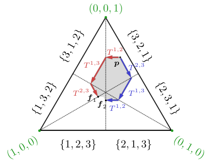
The proof of the above theorem can be found in Appendix B. Before we analyse the complexity of verifying the relation $\bm{p}\ggcurly_{\bm{\gamma}}\bm{q}$ with the use of Theorem 4, let us first illustrate it with an explicit example with $d=3$ and $\bm{\gamma}=(1/3,1/3,1/3)$ (see Fig. 4). In this case, the $\bm{\gamma}$ -ordering is simply the standard sorting in a non-increasing order and $\succ_{\bm{\gamma}}$ coincides with standard majorization $\succ$ . Let us choose $\bm{p}(0)$ with ordering $\{3,2,1\}$ and $\bm{p}(t_{f})$ with ordering $\{1,2,3\}$ . There are then only two canonical sequences from $\bm{\pi}(\bm{p}(0))$ to $\bm{\pi}(\bm{p}(t_{f}))$ :


	$\displaystyle\{3,2,1\}\rightarrow\{2,3,1\}\rightarrow\{2,1,3\}\rightarrow\{1,2,3\},$		(45a)
	$\displaystyle\{3,2,1\}\rightarrow\{3,1,2\}\rightarrow\{1,3,2\}\rightarrow\{1,2,3\}.$		(45b)

For each sequence we construct a final state:


$\displaystyle\bm{f}_{1}$	$\displaystyle=T^{1,2}(1)T^{1,3}(1)T^{2,3}(1)\bm{p}(0),$	(46a)
$\displaystyle\bm{f}_{2}$	$\displaystyle=T^{2,3}(1)T^{1,3}(1)T^{1,2}(1)\bm{p}(0).$	(46b)

According to Theorem 4, $\bm{p}\ggcurly_{{\bm{\gamma}}}\bm{q}$ if and only if either $\bm{f}_{1}\succ_{\bm{\gamma}}\bm{p}(t_{f})$ or $\bm{f}_{2}\succ_{\bm{\gamma}}\bm{p}(t_{f})$ , which is simply a set of $2(d-1)=4$ inequalities. Employing Theorem 1, whenever these inequalities are satisfied there exists a Markovian thermal process mapping $\bm{p}(0)$ to $\bm{p}(t_{f})$ .

The above considerations yield a finite set of inequalities and can hence be checked algorithmically, which in turn means that desideratum (D1) is met. However, how does the approach fare in practice? Taken at face-value, the complexity of the procedure given in Theorem 4 grows extremely quickly with $d$ . To see this, consider a graph whose vertices are all permutations of $\{1,\dots,d\}$ , and whose edges connect strings differing by a transposition of adjacent elements. Then, the number of canonical sequences is equal to the number of simple paths connecting two points on the graph. In the worst-case scenario, an upper bound on this number scales asymptotically as $O(d^{d!})$ . Numerically, we go from $2$ for $d=3$ to over $2000$ for $d=4$ .

An explicit algorithm based on the above theorem will have to adopt a more clever strategy. The general intuition that we will implement in detail in the next section is the following. The theorem mandates to start from $\bm{p}(0)$ and construct all states $\{\bm{f}^{\prime}\}$ corresponding to canonical sequences of length $1$ ; then, each of those is extended to generate all $\{\bm{f}^{\prime\prime}\}$ states corresponding to canonical sequences of length $2$ ; and so on, up to the maximum length $d!-1$ . Crucially, however, we will terminate all paths that are provably worse than those already constructed. If a canonical sequence leads to a state $\bm{f}_{1}$ with a given $\bm{\gamma}$ -ordering, and another leads to a state $\bm{f}_{2}\succ_{\bm{\gamma}}\bm{f}_{1}$ with the same $\bm{\gamma}$ -ordering, the former path will be terminated. This is justified by transitivity of thermomajorization: every state achievable by extending further the path containing $\bm{f}_{1}$ can also be achieved by extending the path containing $\bm{f}_{2}$ , and can thus be removed from the set of conditions in Eq. (44). Pictorially, we will construct an algorithm pushing forward all paths at once, while also constantly monitoring which ones can be terminated.

Intuition suggests that very long paths (of length $O(d!)$ ) are unlikely to be required, since they involve many more thermalizations than the shortest paths connecting $\bm{p}(0)$ to a $\bm{f}$ with the same $\bm{\gamma}$ -ordering as the target $\bm{q}$ . Hence, we expect the algorithm will terminate sequences before they become too long, leading to large savings compared to the worst-case bound. This is confirmed by numerics: for random initial states and random thermal distributions $\bm{\gamma}$ we find that, on average, the longest surviving path to generate every accessible final state has length $L\approx 6.4$ for $d=4$ and $L\approx 11.4$ for $d=5$ . These should be compared with the longest possible paths for $d=4$ (23) and $d=5$ (120). In fact, these $L$ ’s are very close to the length of the shortest sequence connecting two arbitrary points in the above-mentioned graph. This minimal length is equal to $d(d-1)/2$ , so it is $6$ for $d=4$ and $11$ for $d=5$ . The discrepancy can be explained noticing that not all directions in the space of probabilities are “equal”, since the thermal state introduces a thermodynamic asymmetry. Nevertheless, to a first approximation, what the numerics confirm is that Theorem 4 should hold by replacing “enumerate all canonical sequences” with “enumerate all canonical sequences of (close to) minimal length”. This suggests an improved worst-case scaling of $O(d^{d^{2}})$ .⁸⁸ 8 It is however worth emphasising that our algorithm is not using any heuristics: it verifies conditions equivalent to Theorem 4. Here, we are merely discussing how it does so much more quickly that one might naively expect. Finally, numerics also suggest that the path termination procedure is much more efficient than $O(d^{d^{2}})$ scaling: the maximum number of paths $N$ surviving at any point in the algorithm (averaged over random initial conditions and thermal distributions) is $N=9$ for $d=4$ and $N\approx 81.1$ for $d=5$ .

These are the underlying reasons why our algorithm allows one to relatively quickly solve problems up to $d=7$ , which appears prohibitively large if one looks at simple complexity upper bounds. Despite these strong improvements, pushing this dimension up even further will likely require the application of heuristic approaches to the search problem.

VII.2 Constructive protocol

Following Theorem 4, suppose we find a sequence of elementary thermalizations mapping $\bm{p}$ to a final state $\bm{f}$ with the same $\bm{\gamma}$ -ordering as the target $\bm{q}$ and satisfying $\bm{f}\succ_{\bm{\gamma}}\bm{q}$ . Then, one can explicitly construct a sequence of of $M\leq d-1$ elementary thermalizations transforming $\bm{f}$ into $\bm{q}$ (see proof of Theorem 12 in Supplemental Material of Ref. Perry et al. 2018). We thus conclude that a sequence of Markovian thermal processes achieving the transformation from $\bm{p}(0)$ to $\bm{p}(t_{f})=\bm{q}$ is

\bm{q}=\prod_{s=1}^{M}T^{(f_{s},f^{\prime}_{s})}(\lambda_{s})\prod_{k=1}^{N}T^{(i_{k},j_{k})}(1)\bm{p}(0),

(47)

where the first $N$ elementary thermalizations are obtained from a sequence that satisfies Eq. (44), and the construction of the remaining ones can be found in Ref. Perry et al. 2018. This gives an explicit construction involving a sequence of $N+M\leq d!+d-2$ elementary thermalizations achieving any allowed transformation. In other words, Theorem 3 is strengthened to a result that also satisfies desideratum (D2) of Sec. III:

Corollary 5 (Strengthened universality of elementary thermalizations).

$\bm{p}(0)\stackrel{{\scriptstyle\textrm{MTP}}}{{\longmapsto}}\bm{p}(t_{f})$ if and only if there exists a finite sequence of elementary thermalizations such that

\prod_{s=1}^{M}T^{f_{s},f^{\prime}_{s}}(\lambda_{s})\prod_{k=1}^{N}T^{i_{k},j_{k}}(1)\bm{p}(0)=\bm{p}(t_{f}),

(48)

where $N\leq d!-1$ , $M\leq d-1$ and the sequence can be algorithmically constructed.

VII.3 Comparison with previous works

We want to emphasize that the two desiderata considered here, (D1)-(D2) in Sec. III, important as they are to systematically develop and optimize explicit protocols in nonequilibrium thermodynamics, are not typically met by general frameworks. The standard framework based on entropy production provides thermodynamic constraints Landi and Paternostro 2021, but as discussed in Sec. II.2 these are insufficient to characterize the future evolution. Furthermore, these entropic relations do not provide tools to construct and optimize nonequilibrium thermodynamic protocols, unless one focuses on special classes of dynamics, or restricted regimes such as close to equilibrium transformations and slow driving protocols Abiuso et al. 2020. Hence, neither of the two desiderata is satisfied. The same holds true for prominent results in the resource-theoretic approach to thermodynamics. The second laws constraints of Ref. Brandão et al. 2015 are neither finitely checkable, nor they provide a way to construct explicit protocols. The same applies to the “quantum majorization constraints” for thermal processes, the main result derived in Ref. Gour et al. 2018.

Several other settings satisfy desideratum (D1), but not (D2). The framework based on correlating catalysis Lostaglio et al. 2015a; Müller 2018 provides finitely checkable conditions, but not explicit protocols. Similarly, the thermomajorization constraints of Ref. Horodecki and Oppenheim 2013 are finitely checkable by linear programming, but the construction of explicit operations achieving the transformations is not known. More precisely, Ref. Alhambra et al. 2019 did provide a set of thermal processes, called $\beta$ -permutations, whose convex combination realizes the most general transformation. However, beyond the case $d=2$ , it is an open question how these processes can be realized by explicit system-bath interactions. The same is true for the work of Ref. Shiraishi and Sagawa 2021, which provides Gibbs-preserving channels realizing general transformations in the correlating catalyst setting, but not their explicit thermodynamic realization. All these are examples where the desideratum (D2) is not satisfied. Despite noticeable progress Lipka-Bartosik and Skrzypczyk 2021; Henao and Uzdin 2021, the difficulty of satisfying both desiderata has hindered the application of information thermodynamics frameworks.

Ref. Perry et al. 2018 is an exception in this regard, as it provides constructive protocols to realize all the transformations allowed by thermal processes. However, it allows a much more extensive control of the system than we considered here, including full control over its energy spectrum and that of a qubit ancilla. These controls are very powerful: as the authors showed, they allow one to achieve every state transformation possible under thermal processes, including those requiring arbitrary non-Markovian dynamics. Here, instead, we focused on the characterization of thermalizations described by Markovian master equations and involving limited control over the energy spectrum. This paves the way to several applications, as discussed in the accompanying paper Korzekwa and Lostaglio 2022.

VIII Explicit algorithmic verification

Naturally, to verify the complete second laws conditions in higher dimensions, one would like to develop an explicit algorithm that exhaustively verifies the inequalities in Theorem 4. Here we propose one such algorithm with two variants, for which we provide a corresponding Mathematica code Korzekwa 2021. The fast version only verifies whether $\bm{p}(0)\stackrel{{\scriptstyle\textrm{MTP}}}{{\longmapsto}}\bm{p}(t_{f})$ for a fixed initial and final state, while the slow version constructs the set of all final states achievable from a given initial state.

Let us make a few comments on the above algorithm. First, it is clear that it satisfies desideratum (D2) of finite verifiability, but it can be easily modified to also satisfy desideratum (D1) of constructability. One simply needs to keep track of the “history” of each state: in step (2a), one should record which elementary thermalization led to a new state. This history should be kept when updating the optimal states with current states in step (2d). As a result, at the end algorithm we will not only have the list of optimal states within each $\bm{\gamma}$ -ordering, but we will also know the sequence of elementary thermalizations that need to be applied to the initial state to obtain each of them.

Second, the possible number of canonical sequences grows very fast with the system’s dimension $d$ . Thus, one may try to develop heuristics to distinguish between better and worse choices of canonical sequences. Using the example from Fig. 4, it is intuitively clear that in order to go from $\bm{\gamma}$ -ordering $\{1,2,3\}$ to $\bm{\gamma}$ -ordering $\{2,1,3\}$ one should do it directly rather than following the path $\{1,2,3\}\rightarrow\{1,3,2\}\rightarrow\{3,1,2\}\rightarrow\{3,2,1\}\rightarrow\{2,3,1\}\rightarrow\{2,1,3\}$ . Even without any heuristics, we were able to run (on a standard laptop computer) the slow version of the algorithm implemented in Mathematica Korzekwa 2021 to solve the $d=6$ case in minutes and the $d=7$ case in hours.

IX Conclusions and outlook

In this paper we provided a hybrid framework overcoming current limitations of resource-theoretic and master equation approaches to quantum thermodynamics through the novel notion of continuous thermomajorization. Crucially, our approach includes explicit methods to fully solve the question of the existence of a Markovian thermal process mapping between two non-equilibrium states and returns a corresponding sequence of elementary controls when these exist. Exhaustive searches are feasible on a laptop machine up to $d=7$ through the Mathematica code we provided Korzekwa 2021. To achieve this, we employed an exhaustive algorithm (discussed in Sec. VIII) whose strategy appears to effectively cap the maximum sequence length to (close to) the minimum length, while also curbing the number of active sequences at any given time.

While here we tackled the question of describing an algorithm which is guaranteed to provide a definite answer to the interconversion problem, in many circumstances it is enough to find a method that is able to construct useful working protocols in most cases. A promising direction to probe higher-dimensional systems is then to relax the exhaustive search to a heuristic search. For example, if we are interested in states with a target final $\bm{\gamma}$ -order $\bm{\pi}_{f}$ , one could heuristically restricts to canonical sequences that at each step decrease the transposition distance between the current state’s $\bm{\gamma}$ -order $\bm{\pi}_{c}$ and $\bm{\pi}_{f}$ . Another promising direction is to focus on specific task of special relevance, such as cooling. A heuristic protocol is tasked, for example, with decreasing the average energy of the final state. Then, even if an exhaustive search is out of reach, we could run the protocol and terminate it after a given time has passed, or when a given energy target has been met. Coarse-grainings form another direction to be looked at, since we may be interested in the broad properties of the final energy distribution rather than in the exact population in each microscopic energy state. A combination of problem relaxation and heuristic techniques offer, in our opinion, the best way forward to tackling high-dimensional problems.

Pushing the achievable dimension up, and combining the current algorithm optimizing the thermalization stage with alternative methods to optimize unitary stages, will likely open up a range of applications, such as the optimization of quantum thermodynamic cycles of heat engines. In the accompanying paper Korzekwa and Lostaglio 2022 we already discuss ways of employing the framework developed here to construct provably optimal thermodynamic protocols.

At the same time, our framework also offers a rigorous information-theoretical foundation to the dynamical viewpoint of quantum thermodynamics. This approach complements the master equation toolbox, as we have seen, for example, with the systematic construction of generalized entropy production inequalities. Another direction that should be further explored concerns the role of quantum coherence in these settings. We provide some initial remarks in Appendix C, while a solution to this problem satisfying both desiderata (D1)-(D2) is still out of reach.

Acknowledgements

M.L. thanks A. Levy for useful discussions. K.K. acknowledges financial support by the Foundation for Polish Science through TEAM-NET project (contract no. POIR.04.04.00-00-17C1/18-00). M.L. acknowledges financial support from the the European Union’s Marie Skłodowska-Curie individual Fellowships (H2020-MSCA-IF-2017, GA794842), Spanish MINECO (Severo Ochoa SEV-2015-0522 and project QIBEQI FIS2016-80773-P), Fundacio Cellex and Generalitat de Catalunya (CERCA Programme and SGR 875) and grant EQEC No. 682726.

Appendix A Proof of Theorem 1 and Theorem 3

To build up towards our final results we will need several intermediate technical statements. We start by recalling an important result derived in Ref. Perry et al. 2018.

Theorem 6 (Theorem 12, Supplemental Material of Ref. Perry et al. 2018).

If $\bm{p}\succ_{\bm{\gamma}}\bm{q}$ and $\bm{\pi}(\bm{p})=\bm{\pi}(\bm{q})$ , there exists a sequence of elementary thermalizations $\{T^{i_{k},j_{k}}(\lambda_{k})\}_{k=1}^{f}$ such that

T^{i_{f},j_{f}}(\lambda_{f})\dots T^{i_{1},j_{1}}(\lambda_{1})\bm{p}=\bm{q}.

(49)

Moreover, $f\leq d-1$ .

We will also need the following known result characterizing thermomajorization

Theorem 7 (See Refs. Horodecki and Oppenheim 2013; Ruch et al. 1978; Lostaglio 2019).

There exists a stochastic matrix $T$ such that $T\bm{p}=\bm{q}$ and $T\bm{\gamma}=\bm{\gamma}$ if and only if $\bm{p}\succ_{\bm{\gamma}}\bm{q}$ .

Next, we link continuous thermomajorization between two distributions with the existence of a sequence of elementary thermalizations bringing one distribution to another.

Lemma 8 (Continuous thermomajorization and elementary thermalizations).

$\bm{p}\ggcurly_{\bm{\gamma}}\bm{q}$ if and only if there exists a finite sequence of elementary thermalizations $\{T^{i_{k},j_{k}}(\lambda_{k})\}_{k=1}^{f}$ such that

T^{i_{f},j_{f}}(\lambda_{f})\dots T^{i_{1},j_{1}}(\lambda_{1})\bm{p}=\bm{q}.

(50)

Proof.

First, assume $\bm{p}\ggcurly_{\bm{\gamma}}\bm{q}$ . Then, there exists a continuous trajectory $\bm{r}(t)$ with $\bm{r}(0)=\bm{p}$ , $\bm{r}(t_{f})=\bm{q}$ (perhaps $t_{f}=+\infty$ ), and $\bm{r}(t^{\prime})\succ_{\bm{\gamma}}\bm{r}(t^{\prime\prime})$ for all $t^{\prime}\leq t^{\prime\prime}$ . Define $t_{0}=0$ , as well as a thermomajorization ordering $\bm{\pi}^{1}$ and a time $t_{1}$ as follows:


$\displaystyle\bm{\pi}^{1}:=$	$\displaystyle\bm{\pi}(\bm{r}(0)),$	(51a)
$\displaystyle t_{1}:=$	$\displaystyle\sup\{t\|\bm{\pi}(\bm{r}(t))=\bm{\pi}^{1}\}.$	(51b)

Next, for integer $k>1$ , define iteratively


$\displaystyle\bm{\pi}^{k+1}:=$	$\displaystyle\bm{\pi}(\bm{r}(t^{+}_{k})),$	(52a)
$\displaystyle t_{k+1}:=$	$\displaystyle\sup\{t\|\bm{\pi}(\bm{r}(t))=\bm{\pi}^{k+1}\}.$	(52b)

Clearly $t_{k+1}>t_{k}$ . Since there are only $d!$ distinct thermomajorization orderings, ultimately we reach the final $k=f\leq d!-1$ , such that $\bm{\pi}^{f}=\bm{\pi}(\bm{r}(t_{f}))$ . We now employ Theorem 6: for each pair, $\bm{r}(t_{k}^{+})$ and $\bm{r}(t_{k+1})$ , there exists a sequence of elementary thermalizations such that

\bm{r}(t_{k+1})=T^{i_{k_{n}},j_{k_{n}}}(\lambda_{k_{n}})\dots T^{i_{k_{1}},j_{k_{1}}}(\lambda_{k_{1}})\bm{r}(t_{k}),

(53)

with $n\leq d-1$ . Thus, by sequentially applying the above to all $k\leq f$ we obtain Eq. (50) with a finite sequence.

Conversely, assume that Eq. (50) holds. Define $\bm{r}(0)=\bm{p}$ and

\bm{r}(t)=T^{i_{k},j_{k}}(\delta)T^{i_{k-1},j_{k-1}}(\lambda_{k-1})\dots T^{i_{1},j_{1}}(\lambda_{1})\bm{p},

with $k$ and $\delta\in[0,1]$ satisfying $t=\delta+\sum_{i=1}^{k-1}\lambda_{i}$ . This defines a continuous path starting at $\bm{p}$ and terminating at $\bm{q}$ . Moreover, using the fact that for any $i,j$ and $\lambda^{\prime}\geq\lambda$ we can write $T^{i,j}(\lambda^{\prime})=T^{i,j}(\mu)T^{i,j}(\lambda)$ with $\mu\in[0,1]$ , we see that for any $t^{\prime\prime}\geq t^{\prime}$ the distribution $\bm{r}(t^{\prime\prime})$ is obtained from $\bm{r}(t^{\prime})$ by a finite sequence of elementary thermalizations. Given that elementary thermalizations and their products are stochastic matrices with a fixed point $\bm{\gamma}$ , Theorem 7 implies $\bm{r}(t^{\prime})\succ_{\bm{\gamma}}\bm{r}(t^{\prime\prime})$ for all $t^{\prime\prime}\geq t^{\prime}$ . We thus conclude that $\bm{p}\ggcurly_{\bm{\gamma}}\bm{q}$ . ∎

Note that from the proof above one can conclude that the number of elementary thermalizations required for a state transformation is upper-bounded by $d!(d-1)$ , but we will give a tighter bound later. Also, as a corollary of Lemma 8 we get that $\succ_{\bm{\gamma}}$ (describing allowed transformations under general thermal processes, which employ with memory) and $\ggcurly_{\bm{\gamma}}$ (describing allowed transformations under Markovian thermal processes) coincide within a fixed thermomajorization ordering.

Corollary 9.

If $\bm{\pi}(\bm{p})=\bm{\pi}(\bm{q})$ and $\bm{p}\succ_{\bm{\gamma}}\bm{q}$ then $\bm{p}\ggcurly_{\bm{\gamma}}\bm{q}$ . Moreover, the thermomajorizing trajectory $\bm{r}(t)$ connecting $\bm{p}$ to $\bm{q}$ can be chosen such that for all $t\in[0,t_{f}]$ it belongs to the same $\bm{\gamma}$ -ordering.

Proof.

Assuming that $\bm{p}\succ_{\bm{\gamma}}\bm{q}$ and $\bm{\pi}(\bm{p})=\bm{\pi}{(\bm{q})}$ , Theorem 6 tells us then that there exists a sequence of elementary thermalizations mapping $\bm{p}$ into $\bm{q}$ . Using Lemma 8, we conclude $\bm{p}\ggcurly_{\bm{\gamma}}\bm{q}$ . Moreover, the construction of elementary thermalizations presented in the proof of Theorem 6 in Ref. Perry et al. 2018 is such that every intermediate state along the trajectory, $\bm{r}(t)$ , has the same thermomajorization ordering $\bm{\pi}(\bm{p})$ . ∎

We are now able to discuss Theorem 1 and Theorem 3, which we prove jointly as follows:

Theorem 10.

Let $\rho(t)$ by a quantum state with population vector $\bm{p}(t)$ . The following statements are equivalent:

1.

There exists a Markovian thermal process transforming $\rho(0)$ with population $\bm{p}(0)$ into a quantum state $\rho(t_{f})$ with population $\bm{p}(t_{f})$ .
2.

$\bm{p}(0)\ggcurly_{\bm{\gamma}}\bm{p}(t_{f})$ .
3.

There exists a finite sequence of elementary thermalizations such that

$T^{i_{f},j_{f}}(\lambda_{f})\dots T^{i_{1},j_{1}}(\lambda_{1})\bm{p}(0)=\bm{p}(t_{f}).$ (54)

Proof.

Lemma 8 proves the equivalence $2\Leftrightarrow 3$ . To conclude we then just prove $3\Rightarrow 1$ and $1\Rightarrow 2$ .

[ $3\Rightarrow 1$ ]: Given the finite sequence of elementary thermalizations such that Eq. (54) holds, we will explicitly construct a time-dependent Lindbladian $\mathcal{L}_{t}$ generating a Markovian thermal process that maps a state with population $\bm{p}(0)$ to the one with population $\bm{p}(t_{f})$ . We define $\mathcal{L}_{t}$ through its action on the basis elements as

\langle{m}|\mathcal{L}_{t}(\left|n\right\rangle\!\!\left\langle n^{\prime}\right|)|{m^{\prime}}\rangle=\delta_{nn^{\prime}}\delta_{mm^{\prime}}T(t)_{mn}-\delta_{mn}\delta_{m^{\prime}n^{\prime}},

(55)

where $|{x}\rangle$ denote the eigenstates of $H$ and $T(t)$ is a $d\times d$ stochastic matrix. To see that the above $\mathcal{L}_{t}$ corresponds to a valid Lindbladian, note that it has the form $\mathcal{E}_{t}-\mathcal{I}$ , where $\mathcal{I}$ is the identity channel and $\mathcal{E}_{t}$ is the channel that decoheres in the eigenbasis of $H$ and performs the stochastic map $T(t)$ on the diagonal. Since every channel can be written as $\mathcal{E}_{t}(\rho)=\sum_{i}L_{i}\rho L_{i}^{\dagger}$ with $\sum_{i}L_{i}^{\dagger}L_{i}=\mathbb{I}$ , $\mathcal{L}_{t}$ has the required form from Eq. (3).

Next, let

t_{k}=-\log(1-\lambda_{k}),\quad t_{0}:=0

(56)

and introduce $\tau_{k}=\sum_{s=0}^{k}t_{k}$ . Then, choose

T(t)=\begin{bmatrix}\frac{\gamma_{i_{k}}}{\gamma_{i_{k}}+\gamma_{j_{k}}}&\frac{\gamma_{i_{k}}}{\gamma_{i_{k}}+\gamma_{j_{k}}}\\ \\ \frac{\gamma_{j_{k}}}{\gamma_{i_{k}}+\gamma_{j_{k}}}&\frac{\gamma_{j_{k}}}{\gamma_{i_{k}}+\gamma_{j_{k}}}\end{bmatrix}\oplus\bm{0}_{\backslash(i_{k},j_{k})}

(57)

for $t\in\left[\tau_{k-1},\tau_{k}\right]$ with $k=1,\dots,f$ , where $\bm{0}_{\backslash(i_{k},j_{k})}$ denotes the $(d-2)\times(d-2)$ matrix of all zeros acting on the subspace of all energy levels except $i_{k},j_{k}$ . Now, the equation $d\rho/dt=\mathcal{L}_{t}(\rho_{t})$ can be easily solved, and one can verify that the resulting dynamics implements the sequence of elementary thermalizations from Eq. (54) on the population vector. We conclude that a Markovian thermal process mapping $\bm{p}(0)$ into $\bm{p}(t_{f})$ exists.

$[1\Rightarrow 2]:$ Given $\bm{p}(0)$ , $\bm{p}(t_{f})$ and a Markovian thermal process dynamically evolving the former into the latter, let $\bm{p}(t)$ be the trajectory followed at the intermediate times. Employing the definition of an MTP, we have that for every $0\leq t^{\prime}\leq t^{\prime\prime}\leq t_{f}$ there exists a stochastic matrix $T(t^{\prime},t^{\prime\prime})$ such that

T(t^{\prime},t^{\prime\prime})\bm{p}(t^{\prime})=\bm{p}(t^{\prime\prime}),\quad T(t^{\prime},t^{\prime\prime})\bm{\gamma}=\bm{\gamma}.

(58)

From Theorem 7, it follows that $\bm{p}(t^{\prime})\succ_{\bm{\gamma}}\bm{p}(t^{\prime\prime})$ . We conclude that $\bm{p}\ggcurly_{\bm{\gamma}}\bm{q}$ . ∎

Appendix B Proof of Theorem 4

We start from introducing the concept of a coarse-grained description of a thermomajorizing trajectory $\bm{r}(t)$ .

Definition 5 (Coarse-graining).

Let $\bm{r}(t)$ be a thermomajorizing trajectory from $\bm{p}$ to $\bm{q}$ as in Definition 3. Then, a sequence of $\bm{\gamma}$ -orderings $\{\bm{\pi}^{k}\}_{k=1}^{N}$ is called a coarse-grained description of $\bm{r}(t)$ if there exists an ordered set of times $\{t_{k}\}_{k=0}^{N}$ ,

t_{0}=0,\quad t_{k}\leq t_{k+1},\quad t_{N}=t_{f},

(59)

such that the probability vector $\bm{r}(t)$ belongs to the $\bm{\gamma}$ -ordering $\bm{\pi}^{k}$ in the interval $t\in[t_{k-1},t_{k}]$ (note that at time $t_{k}$ , $\bm{r}(t_{k})$ is associated to both $\bm{\gamma}$ -orders $\bm{\pi}^{k}$ and $\bm{\pi}^{k+1}$ ). Moreover, a given coarse-grained description will be called canonical if the sequence $\{\bm{\pi}^{k}\}$ is canonical according to Definition 4.

Note that since a given state can simultaneously belong to more than one $\bm{\gamma}$ -ordering (this happens when $p_{k}/\gamma_{k}=p_{l}/\gamma_{l}$ for some $k$ and $l$ ), the trajectory $\bm{r}(t)$ can have multiple (but finitely many) coarse-grained descriptions. However, as we now prove, we may limit our attention only to canonical coarse-grainings.

Lemma 11.

$\bm{p}\ggcurly_{\bm{\gamma}}\bm{q}$ if and only if there exists a thermomajorizing path $\bm{r}(t)$ connecting $\bm{p}$ and $\bm{q}$ with a canonical coarse-grained description.

Proof.

Assume that $\bm{p}\ggcurly_{\bm{\gamma}}\bm{q}$ , meaning that there exists some thermomajorizing trajectory $\bm{r}(t)$ from $\bm{p}$ to $\bm{q}$ . Since $\bm{r}(t)$ changes continuously in $t$ , so do $\bm{\gamma}$ -rescaled entries $\{r_{i}(t)/\gamma_{i}\}_{i=1}^{d}$ . This means that the $k$ -th largest element among $\bm{\gamma}$ -rescaled entries $\{r_{i}(t)/\gamma_{i}\}_{i=1}^{d}$ becomes equal to the $(k-1)$ -th or $(k+1)$ -th largest one before (or at the same time) becoming equal to any other entry. Hence, we can choose times $\{t_{k}\}_{k=0}^{N}$ (perhaps $t_{k}=t_{k+1}$ for some $k$ ) and assign $\bm{\gamma}$ -orderings $\{\bm{\pi}^{k}\}_{k=1}^{N}$ such that $\bm{\pi}^{k}$ and $\bm{\pi}^{k+1}$ only differ by a transposition of adjacent elements, which proves the first property of the canonical coarse-graining.

To prove the second one, assume that some $\bm{\gamma}$ -ordering $\bm{\pi}$ appears more than once in the coarse-grained description of $\bm{r}(t)$ defined in the previous step. Let us denote the first time $\bm{r}(t)$ has the ordering $\bm{\pi}$ by $t_{1}$ , and the last time it has this ordering by $t_{2}$ . Clearly, $\bm{r}(t_{1})\ggcurly_{\bm{\gamma}}\bm{r}(t_{2})$ . Thus, one can introduce a new thermomajorizing path $\bm{r}^{\prime}(t)$ such that it is equal to $\bm{r}(t)$ for $t\in[0,t_{1})$ and $t\in(t_{2},t_{f}]$ , while for $t\in[t_{1},t_{2}]$ it is the trajectory given by Corollary 9, connecting $\bm{r}(t_{1})$ to $\bm{r}(t_{2})$ and lying completely in $\bm{\gamma}$ -ordering $\bm{\pi}$ . As a result, we obtain a thermomajorizing trajectory $\bm{r}^{\prime}(t)$ connecting $\bm{p}$ and $\bm{q}$ , and such that the $\bm{\gamma}$ -ordering $\bm{\pi}$ appears only once in the coarse-grained description. By repeating this for every $\bm{\gamma}$ -ordering that appears more than once in the original coarse-grained description of $\bm{r}(t)$ , we end up with a trajectory whose coarse-grained description satisfies also the second property of canonical coarse-graining.

Conversely, if there exists a thermomajorizing path $\bm{r}(t)$ connecting $\bm{p}$ and $\bm{q}$ with whatever coarse-grained description, then by definition $\bm{p}\ggcurly_{\bm{\gamma}}\bm{q}$ . ∎

The next lemma geometrically characterizes the action of elementary thermalizations on a Lorenz curve/thermomajorization curve. In words, it shows that the effect of $T^{i,j}$ is to decrease the slope of the $j^{\rm th}$ segment of the thermomajorization curve and increase that of the $i^{\rm th}$ segment till the two are equalized (see Fig. 5 and Appendix B.1 of Ref. Perry et al. 2018).

Figure 5: The defining points of the thermomajorization curve are labelled according to Lemma 12, to visualize the action of the two-level partial level thermalization

T^{3,4}(\lambda)

. This brings down

y_{3}

until, at

\lambda=1

, the slopes of the

3^{rd}

and

4^{th}

segment are equalized (brown segment connecting

2

3^{\prime}

and

4

Lemma 12 (Action of elementary thermalization on the thermomajorization curve).

Consider a Lorenz curve of $\bm{p}$ with elbow points denoted by $(x_{m},y_{m})$ , see Fig. 5. For any $j>i$ , denote $\tilde{i}=\pi_{i}(\bm{p})$ and $\tilde{j}=\pi_{j}(\bm{p})$ . Then, the elementary thermalization $T^{\tilde{i},\tilde{j}}(\lambda)$ shifts down by an equal amount the $y$ -coordinates $(y_{i},\dots,y_{j-1})$ . The extremal map, $T^{\tilde{i},\tilde{j}}(1)$ , equalizes the slopes of the $i^{th}$ and the $j^{th}$ segments of the curve. Note that a final reordering may be needed if the thermomajorization ordering is changed.

Proof.

For $\bm{p}^{\prime}=T^{\tilde{i},\tilde{j}}(\lambda)\bm{p}$ we have

\!\!\!p^{\prime}_{m}=\left\{\begin{array}[]{ll}p_{m}&\textrm{for }m\notin\{\tilde{i},\tilde{j}\},\\ (1-\lambda)p_{m}+\lambda\frac{p_{\tilde{i}}+p_{\tilde{j}}}{\gamma_{\tilde{i}}+\gamma_{\tilde{j}}}\gamma_{m}&\textrm{for }m\in\{\tilde{i},\tilde{j}\}.\end{array}\right.

(60)

Denote by $y_{m}$ and $y^{\prime}_{m}$ the $y$ -coordinates of the thermomajorization curves of $\bm{p}$ and $\bm{p}^{\prime}$ , respectively. Then

y^{\prime}_{m}=\left\{\begin{array}[]{ll}y_{m}&\textrm{for }m<i,\\ y_{m}-\lambda\frac{(p_{\tilde{i}}\gamma_{\tilde{j}}-p_{\tilde{j}}\gamma_{\tilde{i}})}{\gamma_{\tilde{i}}+\gamma_{\tilde{j}}}&\textrm{for }i\leq m<j,\\ y_{m}&\textrm{for }m\geq j.\end{array}\right.

(61)

This corresponds to shifting down the $y$ -coordinate of each point of the thermomajorization curve, starting from the $i^{th}$ point to the $(j-1)^{th}$ point. Setting $\lambda=1$ and using $y_{j}-y_{j-1}=p_{\tilde{j}}$ , one obtains that the slope of the $j^{th}$ segment is

\frac{y^{\prime}_{j}-y^{\prime}_{j-1}}{\gamma_{\tilde{j}}}=\frac{p_{\tilde{i}}+p_{\tilde{j}}}{\gamma_{\tilde{i}}+\gamma_{\tilde{j}}}.

Similarly, the slope of the $i^{th}$ segment is

\frac{y^{\prime}_{i}-y^{\prime}_{i-1}}{\gamma_{\tilde{i}}}=\frac{p_{\tilde{i}}+p_{\tilde{j}}}{\gamma_{\tilde{i}}+\gamma_{\tilde{j}}}.

Hence, the two slopes are equalized for $\lambda=1$ . Note that, if (and only if) $j\neq i+1$ , then the thermomajorization ordering will change at some intermediate $\lambda$ , so that a rearrangement of the segments is necessary to sort them according to non-increasing slopes. ∎

The next lemma identifies states obtained by thermalizing two adjacent levels in the $\bm{\gamma}$ -ordering as the optimal crossings between one ordering and another.

Lemma 13.

Given $\bm{p}$ , we have

T^{\pi_{i}(\bm{p}),\pi_{i+1}(\bm{p})}(1)\bm{p}\ggcurly_{\bm{\gamma}}\bm{q}

(62)

for every $\bm{q}$ satisfying $\bm{p}\ggcurly_{\bm{\gamma}}\bm{q}$ , $\bm{\pi}(\bm{q})=\bm{\pi}(\bm{p})$ and

\frac{q_{\pi_{i}(\bm{p})}}{\gamma_{\pi_{i}(\bm{p})}}=\frac{q_{\pi_{i+1}(\bm{p})}}{\gamma_{\pi_{i+1}(\bm{p})}}.

(63)

Proof.

Since $\bm{p}\ggcurly_{\bm{\gamma}}\bm{q}$ implies $\bm{p}\succ_{\bm{\gamma}}\bm{q}$ , and furthermore we have $\bm{\pi}(\bm{q})=\bm{\pi}(\bm{p})$ , we can use Theorem 6. Its proof shows that there is a sequence of elementary thermalizations such that

\bm{q}=T^{i_{k},j_{k}}(\lambda_{k})\cdots T^{i_{1},j_{1}}(\lambda_{1})\bm{p},

(64)

and, furthermore, that all intermediate states have thermomajorization ordering equal to $\bm{\pi}(\bm{p})$ . Then, we conclude from Lemma 12 that the thermomajorization curve of $\bm{q}$ can be obtained from that of $\bm{p}$ by lowering a set of its $y$ -coordinates while making the slopes of the $i$ -th and $(i+1)$ -th segments equal (no re-orderings are involved, so the $x$ -coordinates do not change).

Now let us focus on $\bm{q}^{i,i+1}:=T^{\pi_{i}(\bm{p}),\pi_{i+1}(\bm{p})}(1)\bm{p}$ . Using again Lemma 12, the thermomajorization curve of the state $\bm{q}^{i,i+1}$ is obtained by lowering the coordinate $y_{i+1}$ till the slopes of the $i$ -th and $(i+1)$ -th segments are equal, while leaving all other $y$ -coordinates untouched. Crucially, note that this is the minimal $y$ -coordinate lowering for any $\bm{q}$ that ensures Eq. (63) is satisfied. From this property and the fact that $\bm{\pi}(\bm{q})=\bm{\pi}(\bm{q}^{i,i+1})$ , it follows that $\bm{q}^{i,i+1}\succ_{\bm{\gamma}}\bm{q}$ . That is because, since $\bm{\pi}(\bm{q})=\bm{\pi}(\bm{q}^{i,i+1})$ implies that the $x$ -coordinates of the thermomajorization curves of $\bm{q}$ and $\bm{q}^{i,i+1}$ coincide, $\succ_{\bm{\gamma}}$ is equivalent to simply comparing the $y$ -coordinates of the respective thermomajorization curves. Using Corollary 9 we conclude $\bm{q}^{i,i+1}\ggcurly_{\bm{\gamma}}\bm{q}$ . ∎

We are now ready to prove the central lemma from which the proof of Theorem 4 follows almost directly.

Lemma 14.

Given a canonical sequence $\{\bm{\pi}^{k}\}_{k=1}^{N}$ with $\bm{\pi}^{1}=\bm{\pi}(\bm{p})$ and $\bm{\pi}^{N}=\bm{\pi}(\bm{q})$ , the following two statements are equivalent:

1.

There exists a thermomajorizing trajectory $\bm{r}(t)$ from $\bm{p}$ to $\bm{q}$ with a canonical coarse-grained description $\{\bm{\pi}^{k}\}_{k=1}^{N}$ .
2.

The following relation holds:

$\prod_{k=1}^{N-1}T^{i_{k},j_{k}}(1)\bm{p}\succ_{\bm{\gamma}}\bm{q},$ (65)

where $T^{i_{k},j_{k}}(1)$ are full thermalizations between levels $i_{k}$ and $j_{k}$ specified by the adjacent elements that differ between $\bm{\pi}^{k}$ and $\bm{\pi}^{k+1}$ .

Proof.

We will prove that the implication holds both ways.

$[1\Rightarrow 2]$ Let $t_{k}$ for $k\in\{0,\dots,N\}$ be the times from Definition 5, i.e., $t_{0}=0$ , $t_{N}=t_{f}$ and the remaining ones describing times for which $\bm{r}(t)$ changes $\bm{\gamma}$ -ordering. By definition, there exist indices $s_{k}$ for $k\in\{1,\dots,N-1\}$ such that $\bm{\pi}^{k}$ and $\bm{\pi}^{k+1}$ differ only by a transposition of the two adjacent entries, $s_{k}$ and $s_{k}+1$ . Let us denote the corresponding energy levels that change order in the $\bm{\gamma}$ -ordering by:

i_{k}:=\pi_{s_{k}}(\bm{r}(t_{k})),\quad j_{k}:=\pi_{s_{k}+1}(\bm{r}(t_{k})).

(66)

By assumption, for $k\in\{0,\dots,N-1\}$ we have $\bm{r}(t_{k})\ggcurly_{\bm{\gamma}}\bm{r}(t_{k+1})$ and

\bm{\pi}(\bm{r}(t_{k}))=\bm{\pi}^{k+1},\quad\bm{\pi}(\bm{r}(t_{k+1}))=\bm{\pi}^{k+1}.

(67)

Furthermore, for $k\in\{0,\dots,N-2\}$

\frac{r(t_{k+1})_{i_{k+1}}}{\gamma_{i_{k+1}}}=\frac{r(t_{k+1})_{j_{k+1}}}{\gamma_{j_{k+1}}}.

(68)

We are then in the conditions to apply Lemma 13 to conclude that for $k\in\{0,\dots,N-2\}$ we have

T^{i_{k+1},j_{k+1}}(1)\bm{r}(t_{k})\ggcurly_{\bm{\gamma}}\bm{r}(t_{k+1}).

(69)

Applying the above sequentially we arrive at

$\displaystyle\bm{r}(t_{N-1})$	$\displaystyle\llcurly_{\bm{\gamma}}T^{i_{N-1},j_{N-1}}(1)\bm{r}(t_{N-2})$
	$\displaystyle\llcurly_{\bm{\gamma}}T^{i_{N-1},j_{N-1}}(1)T^{i_{N-2},j_{N-2}}(1)\bm{r}(t_{N-3})$
	$\displaystyle\llcurly_{\bm{\gamma}}\dots$
	$\displaystyle\llcurly_{\bm{\gamma}}\prod_{k=1}^{N-1}T^{i_{k},j_{k}}(1)\bm{r}(t_{0}=0).$	(70)

Now, recall that $\bm{r}(t_{N-1})\ggcurly_{\bm{\gamma}}\bm{r}(t_{N})=\bm{q}$ and that $\bm{r}(0)=\bm{p}$ . Finally, using transitivity and the fact that relation $\ggcurly_{\bm{\gamma}}$ implies the relation $\succ_{\bm{\gamma}}$ , we conclude that

\prod_{k=1}^{N-1}T^{i_{k},j_{k}}(1)\bm{p}\succ_{\bm{\gamma}}\bm{q}.

(71)

$[2\Rightarrow 1]$ For $t\in[0,N-1]$ define the trajectory

\bm{r}(t)=T^{i_{k},j_{k}}(\delta)T^{i_{k-1},j_{k-1}}(\lambda_{k-1})\dots T^{i_{1},j_{1}}(\lambda_{1})\bm{p},

(72)

with $k$ and $\delta\in[0,1]$ satisfying $t=\delta+\sum_{i=1}^{k-1}\lambda_{i}$ . Note that the resulting trajectory $\bm{r}(t)$ has a coarse-grained description given by $\{\bm{\pi}^{k}\}_{k=1}^{N}$ and that

\bm{p}\ggcurly_{{\bm{\gamma}}}\bm{r}(N-1).

(73)

Now, from the assumption we have that $\bm{r}(N-1)\succ_{\bm{\gamma}}\bm{q}$ and $\bm{\pi}(\bm{r}(N-1))=\bm{\pi}(\bm{q})$ . By Corollary 9 we thus have that $\bm{r}(N-1)\ggcurly_{\bm{\gamma}}\bm{q}$ , and that the trajectory connecting these two states has a fixed $\bm{\gamma}$ -ordering. Hence, $\bm{p}\ggcurly_{{\bm{\gamma}}}\bm{r}(N-1)\ggcurly_{{\bm{\gamma}}}\bm{q}$ and, by transitivity, $\bm{p}\ggcurly_{{\bm{\gamma}}}\bm{q}$ . Therefore, we conclude that there exists a thermomajorizing trajectory from $\bm{p}$ to $\bm{q}$ with a canonical coarse-grained description given by $\{\bm{\pi}^{k}\}_{k=1}^{N}$ . ∎

We are now ready to present the proof of Theorem 4.

Proof.

First, assume that $\bm{p}\ggcurly_{\bm{\gamma}}\bm{q}$ . Then, from Lemma 11, we know that there exists a thermomajorizing path $\bm{r}(t)$ connecting $\bm{p}$ and $\bm{q}$ with some canonical coarse-grained description. Moreover, from Lemma 14 we know that such a path with a given coarse-grained canonical description exists if and only if Eq. (65) is satisfied. Thus, if we list all possible canonical coarse-grained paths connecting $\bm{p}$ and $\bm{q}$ , then for at least one of them Eq. (65) must be satisfied.

Conversely, if Eq. (65) is satisfied for some canonical coarse-grained path, then from Lemma 14 we have $\bm{p}\ggcurly_{\bm{\gamma}}\bm{q}$ . ∎

Appendix C Remarks on fundamental constraints on coherence

In this paper we focused on necessary and sufficient conditions and explicit protocols to generate a given population dynamics. What about the characterization of the evolution of coherences, i.e., the off-diagonal elements of the density matrix in the energy basis? Here we provide some general remarks on this notoriously complex issue.

It has been recognized that the thermodynamic evolution of quantum coherence is restricted by symmetry considerations Lostaglio et al. 2015b. These involve an extension of Noether’s theorem to open quantum system dynamics Marvian and Spekkens 2014. The properties (P1)-(P2) then allow to construct monotonically non-increasing or non-decreasing functionals (monotones) which quantify the deterioration of athermality and coherence during a thermalization process through entropy production-like inequalities. The standard entropy production can be seen as one monotone, to be accompanied by many more which often have independent operational or information-theoretical meaning. Let us briefly discuss some notable examples.

First, we have the $\alpha$ -Rényi entropy production relations:

\forall\alpha\in[0,\infty):\quad\frac{d\Sigma_{\alpha}(t)}{dt}=-\frac{dS_{\alpha}(\rho(t)\|\gamma)}{dt}\geq 0,

(74)

where $\gamma$ is the thermal state from Eq. (4) and $S_{\alpha}$ is the quantum $\alpha$ -Rényi divergence defined by

\!\!S_{\alpha}(\rho\|\sigma)=\left\{\begin{array}[]{ll}\dfrac{\log\mathrm{Tr}\left(\rho^{\alpha}\sigma^{1-\alpha}\right)}{\alpha-1}&\text{~if}\;\alpha\in[0,1),\\ \dfrac{\log\mathrm{Tr}\left(\sigma^{\frac{1-\alpha}{2\alpha}}\rho\sigma^{\frac{1-\alpha}{2\alpha}}\right)}{\alpha-1}&\text{~if}\;\alpha>1,\end{array}\right.

(75)

whose origin in quantum information lies in quantum hypothesis testing Mosonyi and Ogawa 2015. The usual entropy production relation of Eq. (7) is recovered in the limit $\alpha\rightarrow 1$ . Next, we have the $\alpha$ -relative entropy of asymmetry $A_{\alpha}(t)$ Marvian 2012; Lostaglio et al. 2015b,

\!\!\forall\alpha\in[0,\infty):\quad\!\!\!-\frac{dA_{\alpha}(t)}{dt}:=-\frac{dS_{\alpha}(\rho(t)\|\mathcal{D}(\rho))}{dt}\geq 0,

(76)

with $\mathcal{D}$ denoting the dephasing in the energy basis. Asymmetry is a measure of coherence of the state in the basis of $H$ . For $\alpha=1$ the usual entropy production relation can be decomposed as

\frac{d\Sigma(t)}{dt}=\frac{d\Sigma_{d}(t)}{dt}-\frac{dA_{1}(t)}{dt},

(77)

where $\Sigma_{d}=\sum_{i}p_{i}\log(p_{i}/\gamma_{i})$ is the diagonal relative entropy. Hence, $-dA_{1}(t)/dt\geq 0$ can be seen as one of two monotonically non-decreasing additive terms in the standard entropy production equation, measuring the entropic contribution due to loss of quantum coherence Lostaglio et al. 2015b. This constitutes a refinement of the usual entropy production inequality, since both $\Sigma_{d}(t)$ and $-A_{1}(t)$ do not decrease in time, not just their sum Santos et al. 2019. The quantity $A_{1}(t)$ operationally quantifies the coherent contribution in an average work extraction protocol Bäumer et al. 2018, that is the loss to the maximal extractable work due to dephasing of the state. Another example is given by the Fisher information $\mathcal{Q}(\rho(t))$ of the unitary orbit $\{e^{-iH\delta}\rho(t)e^{iH\delta}\}_{\delta\in\mathbb{R}}$ Janzing and Beth 2003; Kwon et al. 2018,

-\frac{d\mathcal{Q}(t)}{dt}\geq 0,

(78)

where

\mathcal{Q}(t)=2-2\lim_{\delta\rightarrow 0}F^{2}[\rho(t),e^{-iH\delta}\rho(t)e^{iH\delta})]

(79)

and $F(\rho,\sigma):=\mathrm{Tr}(\sqrt{\rho^{1/2}\sigma\rho^{1/2}})$ is the quantum fidelity. The quantity $\mathcal{Q}(t)$ measures the information that $\rho(t)$ encodes about the phase along the unitary orbit generated by $H$ , i.e. the metrological value of $\rho(t)$ for phase estimation. Finally, we have the Wigner-Yanase-Dyson skew information Wigner and Yanase 1963; Marvian 2012,

-\frac{dI_{s}(t)}{dt}\geq 0,

(80)

with

I_{s}(t)=-\frac{1}{2}\mathrm{Tr}\left([\rho^{s}(t),H][\rho^{1-s}(t),H]\right),

(81)

where $s\in(0,1)$ . The quantity $I_{s}(t)$ was introduced as a measure of the information contained in measurements that do not commute with $H$ Wigner and Yanase 1963 (for $s=1/2$ one recovers the usual Wigner-Yanase skew information). A systematic framework to deal with all these constructions was developed in Ref. Gour et al. 2018. Leveraging the results obtained there, one can formally define a complete set of monotones. The drawback is that these form an infinite number of extremely involved conditions, and it is not yet clear how these can be simplified.

An alternative approach is to obtain specific computable constraints. For example, exploiting properties (P1)-(P2) and the framework of Ref. Styliaris and Zanardi 2020 (see in particular Eq. (22) therein), one can obtain the following one parameter family of monotones:

\frac{d\mathcal{C}_{\lambda}(t)}{dt}\geq 0,\quad\mathcal{C}_{\lambda}(t)=\frac{-Z(E_{j}-E_{i})^{2}}{\lambda e^{-\beta E_{i}}+e^{-\beta E_{j}}}|C_{ij}(t)|^{2},

(82)

where $C_{ij}(t)$ is the coherence matrix defined in Eq. (14b) and $\lambda\geq 0$ . Note how each coherence element $|C_{ij}(t)|^{2}$ is weighted by a Gibbs factor and the energy difference squared, neatly combining energetic and coherent considerations.

The general problem of Eq. (24) can be explicitly solved for a single qubit system using the minimal decoherence theory of Ref. Lostaglio et al. 2017 (see Sec. E3 therein). However, for higher dimensional systems currently there are no tools to obtain a solution to this problem (perhaps up to some approximation) that satisfies both our fundamental desiderata. We leave this extremely challenging question to future work.

References

Lostaglio (2019) M. Lostaglio, An introductory review of the resource theory approach to thermodynamics, Rep. Prog. Phys. 82, 114001 (2019).
Janzing et al. (2000) D. Janzing, P. Wocjan, R. Zeier, R. Geiss, and T. Beth, Thermodynamic cost of reliability and low temperatures: tightening Landauer’s principle and the second law, Int. J. Theor. Phys. 39, 2717 (2000).
Horodecki and Oppenheim (2013) M. Horodecki and J. Oppenheim, Fundamental limitations for quantum and nanoscale thermodynamics, Nat. Commun. 4, 2059 (2013).
Brandão et al. (2015) F. G. S. L. Brandão, M. Horodecki, N. H. Y. Ng, J. Oppenheim, and S. Wehner, The second laws of quantum thermodynamics, Proc. Natl. Acad. Sci. U.S.A. 112, 3275 (2015).
Ng and Woods (2018) N. H. Y. Ng and M. P. Woods, Resource theory of quantum thermodynamics: Thermal operations and second laws, in Thermodynamics in the Quantum Regime (Springer, 2018) pp. 625–650.
Vinjanampathy and Anders (2016) S. Vinjanampathy and J. Anders, Quantum thermodynamics, Contemp. Phys. 57, 545 (2016).
Kosloff (2013) R. Kosloff, Quantum thermodynamics: A dynamical viewpoint, Entropy 15, 2100 (2013).
Ruch et al. (1978) E. Ruch, R. Schranner, and T. H. Seligman, The mixing distance, J. Chem. Phys. 69 (1978).
Landi and Paternostro (2021) G. T. Landi and M. Paternostro, Irreversible entropy production, from quantum to classical, Rev. Mod. Phys. 93, 035008 (2021).
Korzekwa (2021) K. Korzekwa, Continuous thermomajorisation (2021), github.com/KorzekwaKamil/continuous_thermomajorisation.
Korzekwa and Lostaglio (2022) K. Korzekwa and M. Lostaglio, Optimizing thermalizations, Phys. Rev. Lett. 129, 040602 (2022).
Spaventa et al. (2022) G. Spaventa, S. F. Huelga, and M. B. Plenio, Capacity of non-Markovianity to boost the efficiency of molecular switches, Phys. Rev. A 105, 012420 (2022).
Nielsen and Chuang (2010) M. A. Nielsen and I. L. Chuang, Quantum computation and quantum information (Cambridge university press, 2010).
Breuer and Petruccione (2002) H.-P. Breuer and F. Petruccione, The theory of open quantum systems (Oxford University Press, 2002).
Alicki and Kosloff (2018) R. Alicki and R. Kosloff, Introduction to quantum thermodynamics: History and prospects, in Thermodynamics in the Quantum Regime: Fundamental Aspects and New Directions, edited by F. Binder, L. A. Correa, C. Gogolin, J. Anders, and G. Adesso (Springer International Publishing, Cham, 2018) pp. 1–33.
Gorini et al. (1976) V. Gorini, A. Kossakowski, and E. C. G. Sudarshan, Completely positive dynamical semigroups of N-level systems, J. Math. Phys. 17, 821 (1976).
Lindblad (1976) G. Lindblad, On the generators of quantum dynamical semigroups, Commun. Math. Phys. 48, 119 (1976).
Spohn (1978) H. Spohn, Entropy production for quantum dynamical semigroups, J. Math. Phys. 19, 1227 (1978).
Uzdin et al. (2015) R. Uzdin, A. Levy, and R. Kosloff, Equivalence of quantum heat machines, and quantum-thermodynamic signatures, Phys. Rev. X 5, 031044 (2015).
Campbell et al. (2017) E. T. Campbell, B. M. Terhal, and C. Vuillot, Roads towards fault-tolerant universal quantum computation, Nature 549, 172 (2017).
Klatzow et al. (2019) J. Klatzow, J. N. Becker, P. M. Ledingham, C. Weinzetl, K. T. Kaczmarek, D. J. Saunders, J. Nunn, I. A. Walmsley, R. Uzdin, and E. Poem, Experimental demonstration of quantum effects in the operation of microscopic heat engines, Phys. Rev. Lett. 122, 110601 (2019).
Gour et al. (2018) G. Gour, D. Jennings, F. Buscemi, R. Duan, and I. Marvian, Quantum majorization and a complete set of entropic conditions for quantum thermodynamics, Nat. Commun. 9, 1 (2018).
Brandão et al. (2013) F. G. S. L. Brandão, M. Horodecki, J. Oppenheim, J. M. Renes, and R. W. Spekkens, Resource theory of quantum states out of thermal equilibrium, Phys. Rev. Lett. 111, 250404 (2013).
Perry et al. (2018) C. Perry, P. Ćwikliński, J. Anders, M. Horodecki, and J. Oppenheim, A sufficient set of experimentally implementable thermal operations for small systems, Phys. Rev. X 8, 041049 (2018).
Vom Ende et al. (2019) F. Vom Ende, G. Dirr, M. Keyl, and T. Schulte-Herbrüggen, Reachability in infinite-dimensional unital open quantum systems with switchable gks–lindblad generators, Open Syst. Inf. Dyn. 26, 1950014 (2019).
Schulte-Herbrüggen et al. (2020) T. Schulte-Herbrüggen, F. v. Ende, and G. Dirr, Exploring the limits of open quantum dynamics I: Motivation, new results from toy models to applications, arXiv:2003.06018 (2020).
Renyi (1961) A. Renyi, On measures of entropy and information, in Fourth Berkeley Symposium on Mathematical Statistics and Probability (1961) pp. 547–561.
Elfving (1937) G. Elfving, Zur theorie der Markoffschen ketten, Acta Soc. Sci. Fennicae, n. Ser. A2 8, 1 (1937).
Davies (2010) E. B. Davies, Embeddable Markov matrices, Electron. J. Probab. 15, 1474 (2010).
Kingman (1962) J. F. C. Kingman, The imbedding problem for finite Markov chains, Probab. Theory Relat. Fields 1, 14 (1962).
Runnenburg (1962) J. T. Runnenburg, On Elfving’s problem of imbedding a time-discrete markov chain in a time-continuous one for finitely many states I, P. K. Ned. Akad. A Math 65, 536 (1962).
Goodman (1970) G. S. Goodman, An intrinsic time for non-stationary finite Markov chains, Probab. Theory Relat. Fields 16, 165 (1970).
Carette (1995) P. Carette, Characterizations of embeddable $3\times 3$ stochastic matrices with a negative eigenvalue, New York J. Math 1, 129 (1995).
Marshall et al. (2010) A. W. Marshall, I. Olkin, and B. C. Arnold, Inequalities: Theory of Majorization and Its Applications (Springer, 2010).
Nielsen (2002) M. A. Nielsen, An introduction to majorization and its applications to quantum mechanics, Lecture Notes, Department of Physics, University of Queensland, Australia (2002).
Alhambra et al. (2016) Á. M. Alhambra, J. Oppenheim, and C. Perry, Fluctuating states: What is the probability of a thermodynamical transition?, Phys. Rev. X 6, 041016 (2016).
Zylka (1985) C. Zylka, A note on the attainability of states by equalizing processes, Theoret. Chim. Acta 68, 363 (1985).
Zylka (1990) C. Zylka, On the accessibility of states for systems with dissipative dynamics, Ann. Phys. (Berl.) 502, 268 (1990).
Alberti et al. (2008) P. M. Alberti, B. Crell, A. Uhlmann, and C. Zylka, Order structure (majorization) and irreversible processes, Vernetzte Wissenschaften–Crosslinks in Natural and Social Sciences, PJ Plath, E.-Chr. Hass, eds , 281 (2008).
Hay et al. (2015) M. J. Hay, J. Schiff, and N. J. Fisch, Maximal energy extraction under discrete diffusive exchange, Phys. Plasmas 22, 102108 (2015).
Hay et al. (2017) M. Hay, J. Schiff, and N. J. Fisch, On extreme points of the diffusion polytope, Physica A 473, 225 (2017).
Thon and Wallace (2004) D. Thon and S. W. Wallace, Dalton transfers, inequality and altruism, Soc. Choice Welf. 22, 447 (2004).
Gorban (2013) A. N. Gorban, Thermodynamic tree: The space of admissible paths, SIAM J. Appl. Dyn. Syst. 12, 246 (2013).
Santos et al. (2019) J. P. Santos, L. C. Céleri, G. T. Landi, and M. Paternostro, The role of quantum coherence in non-equilibrium entropy production, npj Quantum Inf. 5, 1 (2019).
Tsallis (1988) C. Tsallis, Possible generalization of boltzmann-gibbs statistics, J. Stat. Phys. 52, 479 (1988).
Abe (2000) S. Abe, Axioms and uniqueness theorem for tsallis entropy, Phys. Lett. A 271, 74 (2000).
Tsallis (2009) C. Tsallis, Introduction to nonextensive statistical mechanics: approaching a complex world (Springer Science & Business Media, 2009).
Mariz (1992) A. M. Mariz, On the irreversible nature of the tsallis and renyi entropies, Phys. Lett. A 165, 409 (1992).
Wilming and Gallego (2017) H. Wilming and R. Gallego, Third law of thermodynamics as a single inequality, Phys. Rev. X 7, 041033 (2017).
Lostaglio et al. (2018) M. Lostaglio, Á. M. Alhambra, and C. Perry, Elementary thermal operations, Quantum 2, 52 (2018).
Mazurek and Horodecki (2018) P. Mazurek and M. Horodecki, Decomposability and convex structure of thermal processes, New J. Phys. 20, 053040 (2018).
Davies (1974) E. B. Davies, Markovian master equations, Commun. Math. Phys. 39, 91 (1974).
Roga et al. (2010) W. Roga, M. Fannes, and K. Życzkowski, Davies maps for qubits and qutrits, Rep. Math. Phys. 66, 311 (2010).
Scarani et al. (2002) V. Scarani, M. Ziman, P. Štelmachovič, N. Gisin, and V. Bužek, Thermalizing quantum machines: Dissipation and entanglement, Phys. Rev. Lett. 88, 097905 (2002).
Bäumer et al. (2019) E. Bäumer, M. Perarnau-Llobet, P. Kammerlander, H. Wilming, and R. Renner, Imperfect thermalizations allow for optimal thermodynamic processes, Quantum 3, 153 (2019).
Miller et al. (2019) H. J. Miller, M. Scandi, J. Anders, and M. Perarnau-Llobet, Work fluctuations in slow processes: quantum signatures and optimal control, Phys. Rev. Lett. 123, 230603 (2019).
Bhatia (2013) R. Bhatia, Matrix analysis, Vol. 169 (Springer Science & Business Media, 2013).
Abiuso et al. (2020) P. Abiuso, H. JD Miller, M. Perarnau-Llobet, and M. Scandi, Geometric optimisation of quantum thermodynamic processes, Entropy 22, 1076 (2020).
Lostaglio et al. (2015a) M. Lostaglio, M. P. Müller, and M. Pastena, Stochastic independence as a resource in small-scale thermodynamics, Phys. Rev. Lett. 115, 150402 (2015a).
Müller (2018) M. P. Müller, Correlating thermal machines and the second law at the nanoscale, Phys. Rev. X 8, 041051 (2018).
Alhambra et al. (2019) Á. M. Alhambra, M. Lostaglio, and C. Perry, Heat-Bath Algorithmic Cooling with optimal thermalization strategies, Quantum 3, 188 (2019).
Shiraishi and Sagawa (2021) N. Shiraishi and T. Sagawa, Quantum thermodynamics of correlated-catalytic state conversion at small scale, Phys. Rev. Lett. 126, 150502 (2021).
Lipka-Bartosik and Skrzypczyk (2021) P. Lipka-Bartosik and P. Skrzypczyk, All states are universal catalysts in quantum thermodynamics, Phys. Rev. X 11, 011061 (2021).
Henao and Uzdin (2021) I. Henao and R. Uzdin, Catalytic transformations with finite-size environments: applications to cooling and thermometry, Quantum 5, 547 (2021).
Lostaglio et al. (2015b) M. Lostaglio, D. Jennings, and T. Rudolph, Description of quantum coherence in thermodynamic processes requires constraints beyond free energy, Nat. Commun. 6, 6383 (2015b).
Marvian and Spekkens (2014) I. Marvian and R. W. Spekkens, Extending Noether’s theorem by quantifying the asymmetry of quantum states, Nat. Commun. 5, 3821 (2014).
Mosonyi and Ogawa (2015) M. Mosonyi and T. Ogawa, Quantum hypothesis testing and the operational interpretation of the quantum rényi relative entropies, Commun. Math. Phys. 334, 1617 (2015).
Marvian (2012) I. Marvian, Symmetry, Asymmetry and Quantum Information, Ph.D. thesis, University of Waterloo (2012).
Bäumer et al. (2018) E. Bäumer, M. Lostaglio, M. Perarnau-Llobet, and R. Sampaio, Fluctuating work in coherent quantum systems: Proposals and limitations, in Thermodynamics in the Quantum Regime (Springer, 2018) pp. 275–300.
Janzing and Beth (2003) D. Janzing and T. Beth, Quasi-order of clocks and their synchronism and quantum bounds for copying timing information, IEEE Trans. Inf. Theory 49, 230 (2003).
Kwon et al. (2018) H. Kwon, H. Jeong, D. Jennings, B. Yadin, and M. S. Kim, Clock–work trade-off relation for coherence in quantum thermodynamics, Phys. Rev. Lett. 120, 150602 (2018).
Wigner and Yanase (1963) E. Wigner and M. M. Yanase, Information contents of distributions, Proc. Natl. Acad. Sci. U.S.A. , 910 (1963).
Styliaris and Zanardi (2020) G. Styliaris and P. Zanardi, Symmetries and monotones in markovian quantum dynamics, Quantum 4, 261 (2020).
Lostaglio et al. (2017) M. Lostaglio, K. Korzekwa, and A. Milne, Markovian evolution of quantum coherence under symmetric dynamics, Phys. Rev. A 96, 032109 (2017).

Continuous thermomajorization and a complete set of laws for Markovian thermal processes

Abstract

I Introduction

II Setting the scene

II.1 Thermodynamic frameworks

II.1.1 The traditional approach

Definition 1.

II.1.2 The resource-theoretic approach

Definition 2.

II.1.3 Potential and need for generalizations of the MTP model

II.2 Insufficiency of current approaches

II.2.1 Insufficiency of the traditional approach

II.2.2 Insufficiency of the resource-theoretic approach

III Proposed hybrid approach

IV Continuous thermomajorization

IV.1 Recap: majorization and thermomajorization

IV.2 Continuous thermomajorization

Definition 3 (Continuous thermomajorization).

Theorem 1 (Second law on populations).

V A complete set of entropy production relations

Proof.

Corollary 2 (Exhaustive HH-type theorem).

Proof.

VI Universal thermodynamic controls

Theorem 3 (Universality of elementary thermalizations).

VII Second laws in the Markovian regime

VII.1 Finite set of conditions

Definition 4.

Theorem 4 (Finite second laws conditions).

VII.2 Constructive protocol

Corollary 5 (Strengthened universality of elementary thermalizations).

VII.3 Comparison with previous works

VIII Explicit algorithmic verification

IX Conclusions and outlook

Acknowledgements

Appendix A Proof of Theorem 1 and Theorem 3

Theorem 6 (Theorem 12, Supplemental Material of Ref. Perry et al. 2018).

Theorem 7 (See Refs. Horodecki and Oppenheim 2013; Ruch et al. 1978; Lostaglio 2019).

Lemma 8 (Continuous thermomajorization and elementary thermalizations).

Proof.

Corollary 9.

Proof.

Theorem 10.

Proof.

Appendix B Proof of Theorem 4

Definition 5 (Coarse-graining).

Lemma 11.

Proof.

Lemma 12 (Action of elementary thermalization on the thermomajorization curve).

Proof.

Lemma 13.

Proof.

Lemma 14.

Proof.

Proof.

Appendix C Remarks on fundamental constraints on coherence

References

Continuous thermomajorization and a complete set of laws
for Markovian thermal processes

Corollary 2 (Exhaustive $H$ -type theorem).