Self-Supervised Pre-Training for Transformer-Based Person Re-Identification
Abstract
Transformer-based supervised pre-training achieves great performance in person re-identification (ReID). However, due to the domain gap between ImageNet and ReID datasets, it usually needs a larger pre-training dataset (e.g. ImageNet-21K) to boost the performance because of the strong data fitting ability of the transformer. To address this challenge, this work targets to mitigate the gap between the pre-training and ReID datasets from the perspective of data and model structure, respectively. We first investigate self-supervised learning (SSL) methods with Vision Transformer (ViT) pretrained on unlabelled person images (the LUPerson dataset), and empirically find it significantly surpasses ImageNet supervised pre-training models on ReID tasks. To further reduce the domain gap and accelerate the pre-training, the Catastrophic Forgetting Score (CFS) is proposed to evaluate the gap between pre-training and fine-tuning data. Based on CFS, a subset is selected via sampling relevant data close to the down-stream ReID data and filtering irrelevant data from the pre-training dataset. For the model structure, a ReID-specific module named IBN-based convolution stem (ICS) is proposed to bridge the domain gap by learning more invariant features. Extensive experiments have been conducted to fine-tune the pre-training models under supervised learning, unsupervised domain adaptation (UDA), and unsupervised learning (USL) settings. We successfully downscale the LUPerson dataset to 50% with no performance degradation. Finally, we achieve state-of-the-art performance on Market-1501 and MSMT17. For example, our ViT-S/16 achieves 91.3%/89.9%/89.6% mAP accuracy on Market1501 for supervised/UDA/USL ReID. Codes and models will be released to https://github.com/michuanhaohao/TransReID-SSL.
1 Introduction
Transformer-based methods he2021transreid; zhang2021hat have attracted more and more attention and achieved great performance in person ReID. For example, the pure transformer-based method TransReID he2021transreid achieves a significant performance boost over state-of-the-art CNN-based methods. However, there exists a large domain gap between ImageNet and person ReID datasets because 1) The image content of ImageNet and ReID datasets is very different fu2021unsupervised; 2) supervised pre-training on ImageNet is focused on category-level supervision which reduces the rich visual information dino while person ReID prefers fine-grained identity information. As a result, Transformers need to be pre-trained on a larger-scale dataset ImageNet-21K deng2009imagenet to avoid over-fitting on the pre-training dataset. To bridge the gap between pre-training and fine-tuning datasets for better transformer-based ReID models, this paper tackles the problem from the perspectives of data and model structure, respectively.
From the data view, we have seen a large-scale pre-training dataset named LUPerson being built by collecting unlabeled person images fu2021unsupervised, which has demonstrated that CNN-based SSL pre-training on LUPerson dataset improves ReID performance compared with ImageNet-1k pre-traininng. However, following the same paradigm and replacing the backbone with Vision Transformers (ViTs) VIT would get poor performance due to the huge differences between training CNNs and ViTs. It motivates us to explore an effective SSL pre-training paradigm for transformer-based person ReID in the first place. After thorough comparison between several Transformer-based self-supervised methods (e.g. MocoV3 chen2021mocov3, MoBY moby and DINO dino) with ViTs on the LUPerson dataset, it is found that DINO significantly outperforms other SSL methods and supervised pre-training on ImageNet, thus it is used as our following setup. Next, it is brought to our attention that, though with better performance, pre-training on LUPersonn needs a larger amount of computational resources due to the large amount of training data (3X of ImageNet-1K). Therefore, we propose to adopt conditional pre-training to speed-up the training process and further reduce the domain gap. As LUPerson is collected from web videos, a portion of the images are of low-quality or have great domain bias with the downstream ReID datasets, so conditional filtering shall be performed to downscale LUPerson (source domain) by selecting a relevant subset close to the downstream ReID datasets (target domain). However, previous works on conditional filtering chakraborty2020efficient; coleman2020selection; ge2017borrowing; cui2018large; Fine are mainly designed for close-set tasks by selecting data close to category labels or cluster centers of the target training data. Those methods will easily overfit the person IDs instead of the true target domain if directly applied to the open-set ReID task. We propose a metric named Catastrophic Forgetting Score (CFS) to evaluate the gap between pre-training and downstream data, inspired by the conclusions in catastrophic forgetting problems thompson2019overcoming; kirkpatrick2017overcoming; ramasesh2021anatomy. For a pre-training image, the similarity between its features from the two proxy models (one is pre-trained on the source dataset and another is fine-tuned on the target dataset) can represent the similarity between the source and target domain. In this way, a subset of images with higher CFS scores can be selected from the pre-training data to perform efficient conditional pre-training. A preliminary theoretical analysis is conducted to justify the effectiveness of CFS.
From the perspective of model structure, some recent works chen2021mocov3; conv_stem; wang2021scaled have pointed out that, an important factor that affects performance and stability of ViTs is the patchify stem implemented by a stride- convolution ( by default) on the input image. To address this problem, MocoV3 chen2021mocov3 froze the patch projection to train ViTs, while Xiao et al. conv_stem and Wang et al. wang2021scaled proposed a convolution stem stacked by several convolution, Batch Normalization (BN) bn, and ReLU relu layers to increase optimization stability and improve performance. Inspired by the success of integrating Instance Normalization (IN) and BN to learn domain-invariant representation in the ReID task BoT; ibnnet; dai2021cluster, we refer to IBN-Net ibnnet and improve the convolution stem to the IBN-based convolution stem (ICS). ICS inherits the stability of the convolution stem and also introduces IBN to learn features with appearance invariance (e.g. viewpoint, pose and illumination invariance, etc.). ICS has similar computational complexity to convolution stem, but improves peak performance of ViTs significantly in person ReID.
Embraced with the above two improvements based on DINO, we conduct experiments with supervised learning, UDA and USL settings on Market1501 and MSMT17. Our pre-training paradigm helps ViTs achieve state-of-the-art performance on these benchmarks. For instance, as shown in Figure 1, our ViT-S achieves 91.3%/89.9%/89.6% mAP accuracy on Market-1501 for supervised/UDA/USL ReID, which exceed the supervised pre-training setting on ImageNet by a large margin. The pre-training cost on LUPerson is also reduced by 30% without any performance degradation, through the proposed CFS-based conditional filtering and downscaling the original LUPerson by 50%.
2 Related Works
2.1 Self-supervised Learning
Self-supervised learning (SSL) methods are proposed to learn discriminative features from large-scale unlabeled data without any human-annotated labels jing2020self. One branch is developed from Momentum Contrast (MoCo) moco_v2 by treating a pair of augmentations of a sample as a positive pair and all other samples as negative pairs. Since the number of negative samples greatly affects the final performance, MoCo series chen2021mocov3; moco_v2 require large batches or memory banks. Among them, MoCoV3 chen2021mocov3 is a Transformer-specific version. Fu et al. fu2021unsupervised have verified ResNet50 can be well pre-trained by a modified MoCoV2 on human images in person ReID. Many recent works have shown models can learn feature representation without discriminating between images. In this direction, Ge et al. BYOL propose a new paradigm called BYOL, where the online network predicts the representation of the target network on the same image under a different augmented view. Large batch size is unnecessary in BYOL since negative samples are not needed. Many variants have successfully improved BYOL in various ways. One of them is DINO dino, where a centering and sharpening of the momentum teacher outputs is used to avoid model collapse. DINO achieves state-of-the-art performance with ViTs on both ImageNet classification and down-stream tasks. Xie et al. combines MoCo with BOYL to propose a Transformer-specific method called MoBY. Given that there have been more SSL methods designed specifically for Transformers, we will focus on several of the state-of-the-art options in the following experiments, e.g. MoCo series, MoBY and DINO.
2.2 Transformer-based ReID
CNN-based methods have dominated the ReID community for many years. However, pure-transformer models are gradually becoming a popular choice. He et al. he2021transreid are the first to successfully apply ViTs to ReID tasks by proposing TransReID which achieves state-of-the-art performance on both person and vehicle ReID. Auto-Aligned Transformer (AAformer) zhu2021aaformer also uses ViT backbone with the additional learnable vectors of “part tokens” to learn the part representations and integrates the part alignment into the self-attention. Other works try to use Transformer to aggregate features or information from CNN backbones. For example, zhang2021hat; shen2021git; PAT integrate Transformer layers into the CNN backbone to aggregate hierarchical features and align local features. For video ReID, zhang2021spatiotemporal; liu2021video exploit Transformer to aggregate appearance features, spatial features, and temporal features to learn a discriminative representation for a person tracklet.
2.3 Conditional Transfer Learning
There are a few works chakraborty2020efficient; coleman2020selection; ge2017borrowing; cui2018large; Fine; yan2020neural studying how to select relevant subsets from the pre-training dataset to improve the performance when transferred to target datasets. cui2018large use a feature extractor trained on the JFT300M hinton2015distilling to select the most similar source categories to the target categories in a greedy way. For each image from the target domain, Ge et al. ge2017borrowing search a certain number of images with similar low-level characteristics from the source domain. Shuvam et al. chakraborty2020efficient train the feature extractor on the target data and individually select source images that are close to cluster centers in the target domain. Yan et al. yan2020neural propose a Neural Data Server (NDS) to train expert models on many subsets of the pre-training dataset. Source images used to train an expert with a good target task performance are assigned high importance scores. It is noted that conditional transfer learning has mainly been studied on close-set tasks such as image classification, fine-grained recognition, object detection, etc. Therefore, these methods may be not suitable for the open-set ReID task.
3 Self-supervised Pre-training
As far as we know, there has been no literature studying the SSL pre-training for transformer-based ReID. Therefore we first conduct an empirical study to gain better understanding on this problem. We investigate two backbones (CNN-based ResNet50 and Transformer-based ViT), four SSL methods (MoCoV2, MoCoV3, MoBY and DINO), and two pre-training datasets (ImageNet and LUPerson). MoCoV2 used here is a modified version proposed to adapt to person ReID on ResNet50 in fu2021unsupervised, while the other three methods, i.e. MoCoV3, MoBy and DINO, are transformer-specific methods proposed on the ImageNet data.
3.1 Supervised Fine-tuning
| Pre-training | Market | MSMT17 | ||||
|---|---|---|---|---|---|---|
| Models | Methods | Data | mAP | R1 | mAP | R1 |
| R50 | Supervised | IMG | 86.7 | 94.8 | 52.2 | 76.0 |
| MoCoV2 | LUP | 88.2 | 94.8 | 53.3 | 76.0 | |
| MoCoV3 | LUP | 87.3 | 95.1 | 52.9 | 76.8 | |
| DINO | LUP | 86.5 | 94.4 | 51.9 | 75.8 | |
| ViT-S/16 | Supervised | IMG | 85.0 | 93.8 | 53.5 | 75.2 |
| MoCoV2 | IMG | 63.6 | 72.1 | 19.6 | 36.1 | |
| MoCoV3 | IMG | 81.7 | 92.1 | 46.6 | 70.3 | |
| MoBY | IMG | 83.3 | 92.2 | 49.1 | 71.5 | |
| DINO | IMG | 84.6 | 93.1 | 54.8 | 76.7 | |
| ViT-S/16 | MoCoV2 | LUP | 72.1 | 87.6 | 27.8 | 47.4 |
| MoCoV3 | LUP | 82.2 | 92.1 | 47.4 | 70.3 | |
| MoBY | LUP | 84.0 | 92.9 | 50.0 | 73.2 | |
| DINO | LUP | 90.3 | 95.4 | 64.2 | 83.4 | |
| DINO | LUP∗ | 89.6 | 95.1 | 62.3 | 82.6 | |
The baseline he2021transreid we used is pre-trained on ImageNet. We fine-tune pre-trained models on two ReID benchmarks including Market-1501 (Market) and MSMT17, and the peak fine-tuning performance of all models being compared are presented in Table 1. For convenience, a pre-trained model is marked in the form of Model+Method+Data. For instance, R50+Supervised+IMG denotes the ResNet50 model pre-trained on the ImageNet in the supervised manner, which is the standard pre-training paradigm in most previous ReID methods.
Some observations are made as follows. 1) MoCoV2 performs the best among all SSL methods for ResNet50, while it is much worse than the other three transformer-specific methods with ViT, which means that it is necessary to explore specific methods for transformer-based models. 2) ViT is more sensitive to a proper pre-training than ResNet50. For example, we can see that mAP using ResNet50 ranges from 51.9% to 53.3% on MSMT17 with different pre-training settings, while performance of ViT-S/16 differs more widely on MSMT17. 3) SSL methods on LUP consistently achieve better performance comparing to SSL with ImageNet. Even when we restrict the number of training images of LUP to be the same as IMG, ViT-S/16+DINO+LUP∗ still surpasses ViT-S/16+DINO+ IMG on both benchmarks, indicating that leveraging person images is a better choice to pre-train ReID models. 4) ViT-S/16+DINO+LUP achieves 64.2% mAP and 83.4% Rank-1 accuracy on the MSMT17, surpassing the baseline (ViT-S/16+Supervised+IMG) by 10.7% mAP and 8.2% Rank-1 accuracy.
3.2 Unsupervised Fine-tuning
| Pre-training | Market | MSMT17 | ||||
|---|---|---|---|---|---|---|
| Models | Methods | Data | mAP | R1 | mAP | R1 |
| R50 | Sup | IMG | 82.6 | 93.0 | 33.1 | 63.3 |
| SSL | LUP | 84.0 | 93.4 | 31.4 | 58.8 | |
| ViT-S/16 | Sup | IMG | 62.5 | 80.5 | 13.5 | 29.9 |
| SSL | IMG | 68.9(+6.4) | 84.3(+3.8) | 14.9(+1.4) | 31.0(+1.1) | |
| SSL | LUP | 87.8(+25.3) | 94.4(+13.9) | 38.4(+24.9) | 63.8(+33.9) | |
| Pre-training | MS2MA | MA2MS | ||||
|---|---|---|---|---|---|---|
| Models | Methods | Data | mAP | R1 | mAP | R1 |
| R50 | Sup | IMG | 82.4 | 92.5 | 33.4 | 60.5 |
| SSL | LUP | 85.1 | 94.4 | 28.3 | 53.8 | |
| ViT-S/16 | Sup | IMG | 68.5 | 85.4 | 13.6 | 29.5 |
| SSL | IMG | 79.7(+11.2) | 90.5(+5.1) | 21.8(+8.2) | 41.6(+12.1) | |
| SSL | LUP | 88.5(+20.0) | 95.0(+9.6) | 43.9(+30.3) | 67.7(+38.2) | |
Since there has been no transformer-based baseline for unsupervised ReID, the state-of-the-art CNN-based framework C-Contrast dai2021cluster is selected for the following experiments. We reproduce C-Contrast with ResNet50 and ViT-S/16 on both USL ReID and UDA ReID 11 1 https://github.com/alibaba/cluster-contrast-reid. All results are reproduced using the official code with the same random seed and GPU machine to reduce randomness.. Based on observations made from Table 1, we choose MoCoV2 for ResNet50 and DINO for ViT-S/16 in this section in Table 2. SSL pre-training doesn’t provide large gains compared with Sup when applied with ResNet50, not to mention that performance drop is observed on MSMT17. This is consistent with the aforementioned conclusion that Transformer is more sensitive to the pre-training than CNN. In contrast, SSL pre-training on LUPerson improves the performance by a large margin for ViT-S/16. The UDA performance on MS2MA and MA2MS also yields the similar conclusion.
Conclusion. DINO is the most suitable SSL method among candidate methods for transformer-based ReID. Pre-training is more crucial for Transformers than CNN models. Transformers pre-trained on LUPerson can significantly improve the performance compared with ImageNet pre-training, indicating that bridging the domain gap between pre-training and fine-tuning datasets for transformers is more beneficial and worth doing.
4 Conditional Pre-training
This section introduces the efficient conditional pre-training where models are pre-trained on a subset closer to the target domain to speed up the pre-training process while maintaining or even improving the downstream fine-tuning performance. Catastrophic Forgetting Score (CFS) is proposed to evaluate the similarity between the pre-training data and the target domain. Theoretic analysis is provided to support the method.
4.1 Problem Definition
Given a target dataset where with their ID labels . We target to select a subset from a large-scale source/pre-training dataset where . The number of images in is . The efficient conditional pre-training is to pre-train models on , which should reduce the training cost of pre-training while maintaining or even improving performance on the target dataset. Some previous works chakraborty2020efficient; coleman2020selection; Fine have shown that the solution is to select pre-training data close to the target domain, and we also provide theoretical analysis in Appendix to further verify this. Since ReID is a open set problem with different IDs in training and testing set, the key problem is how to design a metric to evaluate the ‘similarity’ between the pre-training data and the target dataset (instead of the person IDs in ).
4.2 Catastrophic Forgetting Score
We first pre-train a model on the source dataset . is transferred into by fine-tuning on the target dataset . Since and only serve as proxy models to select data, there is no need for them to achieve the best ReID performance, i.e. they can be lightweight models trained with less epochs. In this paper, is the fusion of Market-1501 and MSMT17, so we only need to select one subset sharing between different ReID datasets.
Many previous works thompson2019overcoming; kirkpatrick2017overcoming; ramasesh2021anatomy have observed that catastrophic forgetting in neural networks occurs during domain transferring, and the degree of forgetting is related to the gap between the source domain and the target domain. To evaluate the domain gap between the pre-training data and the target domain, a simple metric named Catastrophic Forgetting Score (CFS) is proposed as below, which computes the representation similarity between and for the pre-training data :
| (1) |
The greater the , the smaller the degree of forgetting, i.e. the smaller the domain gap. is sorted in descending order and the top images are selected to get the subset .
The advantage of CFS is that it does not compare directly with the images in the target domain. That is, unlike previous methods designed for close-set tasks, it avoids scanning through all images from the target domain to compute , which is computationally costly.
4.3 Theoretical Analysis of CFS
In this subsection, we give a theoretical analysis to show large CFS is a necessary condition for finding an image in the source domain that is close to the target domain. To this end, we first rigorously define some terminologies as follows, which will be used in the analysis.
Definition 1.
The feature representation is a function of that maps to , i.e., .
The feature representation is a function extracting features of an image. Without loss of generality, we use the normalized representation function in our analysis, i.e.,
| (2) |
where is the norm.
Definition 2.
We say and are -similar, if , where is a small constant, and are two representation functions, and are defined as (2). In addition, if , we use -similar for simplicity.
The similarity of two images can be defined as the “closeness” of their features. This is reasonable since the feature is considered as the representation of an image.
Assumption 1.
If and are close, then they are -similar, i.e., , where and are two representation functions, and are defined as (2).
Since our inference focuses on downstream tasks, it is interested in considering the representation for the target domain (i.e., ). The main goal is to find an image in the source domain that is -similar to an image from the target domain. Mathematically, we aim to find to be -similar to 22 2 Please note that could not be a true image from target domain and it is for the proof use only. In general, the image can be a virtual one that follows the same distribution of the images of target domain., that is,
| (3) |
The following theorem shows that the large CFS is a necessary condition for finding such an image in the source domain.
Theorem 1.
Proof.
Let define the distance
| (5) |
We write the distance as
| (6) |
where the last inequality uses Triangle Inequality for norm. Furthermore, if and are close, then under Assumption 1 we have
| (7) |
Next, we want to explain why the small distance can be used as the selection criterion, let consider two cases. When , by (5) and (4.3) we have
| (8) |
When , by (4.3) and (7), we have
| (9) |
Thus, if the distance , then by (8) and (9) we know and are -similar, i.e., (3) holds.
The above condition of is equivalent to (4) since . So the greater is, the smaller is. ∎
Although larger value of CFS is proved to be only a necessary condition for finding a source domain image close to the downstream task, Table 5 also empirically shows that this metric is effective in practice.
5 IBN-based Convolution Stem
Our architecture design is based on two important experiences. 1) The patchity stem implemented by a stride- convolution ( by default) in the standard ViT is the key reason of training instability chen2021mocov3. Recent works show the convolution stem conv_stem; wang2021scaled stacked with several convolution, BN and ReLU layers can significantly improve training stability and peak performance. 2) Data bias is a critical challenge for person ReID. By learning invariant representation, IBNNet-a block ibnnet has achieved a huge success in many publications or academic challenges luo2019strong; dai2021cluster.
When applying ViTs in ReID tasks, a straightforward way is to introduce IBNNet-a block into the convolution stem. Following the original design of IBNNet-a, we propose IBN-based convolution stem (ICS), as shown in Figure 2, by applying BN for half of the channels and IN for the other half after shallow convolution layers, and applying only BN layers after deep convolution layers. In this paper, we choose to apply IN after the first two convolution layers. Another variant worth consideration but may slightly reduce performance is to only apply IN after the first convolution layer. The kernel sizes, channels and strides of the convolution stem are kept the same as in conv_stem. Hereinafter, we denote ViT with patchify stem, convolution stem, and ICS as ViT, ViTC and ViTI, respectively
6 Experiments
6.1 Implementation Details
Datasets. The dataset used for pre-training, LUPerson fu2021unsupervised, contains 4.18M unlabeled human images in total, collected from 50,534 online videos. To evaluate the performance on ReID tasks, we conduct experiments on two popular benchmarks, i.e. Market-1501 (Market) Market1501 and MSMT17 MSMT17. They contain 32,668 images of 1,501 identities and 126,441 images of 4,101 identities, respectively. Images in these two datasets are resized to during training and inference stages. Standard evaluation protocols are used with the metrics of mean Average Precision (mAP) and Rank-1 accuracy.
Pre-training. Unless otherwise specified, we follow the default training settings of all self-supervised methods. Images are resized to and for ImageNet and LUPerson, respectively. For pre-training on LUPerson with DINO, the model is trained on V100 GPUs for 100 epochs and a multi-crop strategy is applied to crop 8 images with resolution.
Supervised ReID. The transformer-based baseline proposed in he2021transreid is used as our baseline in this paper. That is to say, none of the overlapping patch embedding, jigsaw patch module or side information embedding is included here. It is noticed that DINO models should be fine-tuned with a small learning rate and a longer warm-up process, so we recommend setting the learning rate to and warm-up epochs to be 20. All other settings are same with the original paper.
USL/UDA ReID. We follow most of the default settings in dai2021cluster. USL ReID and UDA ReID share the same training settings in this paper, and the only difference is that the models for UDA ReID need to be first pre-trained on source datasets before training in an unsupervised manner on target datasets. The maximum distance between two samples is set to 0.6 and 0.7 for Market1501 and MSMT17, respectively. We use SGD optimizer to train ViTs for 50 epochs. The initial learning rate is set to 3.5e-4, and is reduced 10 times for every 20 epochs. Each mini-batch contains 256 images of 32 person IDs, i.e. each ID contains 8 images. The rate of stochastic depth is set 0.3.
6.2 Results of Conditional Pre-training
| Pre-training | Market | MSMT17 | ||
|---|---|---|---|---|
| mAP | R1 | mAP | R1 | |
| Full (100%) | 90.3 | 95.4 | 64.2 | 83.4 |
| Random (50%) | 89.9 | 95.2 | 62.9 | 82.6 |
| Cluster (50%) chakraborty2020efficient | 90.0 | 95.4 | 63.8 | 83.3 |
| CFS (50%) | 91.0 | 96.0 | 66.1 | 84.6 |
| Pre-training | Market | MSMT17 | ||
|---|---|---|---|---|
| mAP | R1 | mAP | R1 | |
| MocoV2+R50 fu2021unsupervised | 88.2 | 94.8 | 53.3 | 76.0 |
| +CFS (50%) | 89.4 | 95.5 | 56.8 | 78.8 |
| DINO+ViT-S | 90.3 | 95.4 | 64.2 | 83.4 |
| +CFS (50%) | 91.0 | 96.0 | 66.1 | 84.6 |
| Supervised ReID | USL ReID | UDA ReID | |||||||||||
|---|---|---|---|---|---|---|---|---|---|---|---|---|---|
| Pre-training | Market | MSMT17 | Market | MSMT17 | MS2MA | MA2MS | |||||||
| Data | Model | mAP | R1 | mAP | R1 | mAP | R1 | mAP | R1 | mAP | R1 | mAP | R1 |
| Full (100%) | ViT-S/16 | 90.3 | 95.4 | 64.2 | 83.4 | 87.8 | 94.4 | 38.4 | 63.8 | 88.5 | 95.0 | 43.9 | 67.7 |
| ViTC-S/16 | 90.7 | 95.7 | 65.2 | 84.5 | 88.3 | 94.6 | 39.7 | 65.2 | 89.1 | 95.3 | 49.0 | 73.4 | |
| ViTI-S/16 | 91.1 | 95.9 | 66.8 | 85.5 | 89.3 | 94.8 | 48.8 | 74.4 | 89.6 | 95.6 | 55.0 | 77.9 | |
| +0.8 | +0.5 | +2.6 | +2.1 | +1.5 | +0.4 | +10.4 | +10.6 | +1.1 | +0.6 | +11.1 | +10.2 | ||
| CFS (50%) | ViT-S/16 | 91.0 | 96.0 | 66.1 | 84.6 | 88.2 | 94.2 | 40.9 | 66.4 | 89.4 | 95.4 | 47.4 | 70.8 |
| ViTC-S/16 | 91.2 | 95.8 | 67.8 | 85.7 | 89.3 | 95.0 | 42.5 | 67.6 | 89.7 | 95.5 | 55.7 | 75.5 | |
| ViTI-S/16 | 91.3 | 96.2 | 68.1 | 86.1 | 89.6 | 95.3 | 50.6 | 75.0 | 89.9 | 95.5 | 57.8 | 79.5 | |
| +0.3 | +0.2 | +2.0 | +2.5 | +1.4 | +0.9 | +9.7 | +8.6 | +0.5 | +0.1 | +10.4 | +8.7 | ||
Effect of partial data. As shown in Figure 3, pre-training with 30% data achieves comparable performance with the full-data pre-training. It is surprising that 40%60% pre-training data even improves the performance slightly(e.g. 66.3% vs 64.2% mAP on MSMT17). Therefore, filtering irrelevant data with CFS from the pre-training data is actually beneficial instead of harmful to the down-stream performance. For a better trade-off between accuracy and pre-training cost, 50% of the pre-training data will be sampled in our following experiments.
Time consumption of pre-training. Although our conditional pre-training is two-stage, it is still more efficient. Standard pre-training of a ViT-S on full LUPerson takes 107 hours with 8V100 GPUs. In our conditional pre-training, data selection step takes 21 hours because the proxy models only need to be pre-trained for 20 epochs. For the second stage, pre-training the model on 50% of LUPerson only takes 51 hours. In total we can still save about 30% of pre-training time with a slight performance improvement.
Selection strategies. Different selection strategies are compared in Table 5. Randomly sampling 50% data for pre-training does not help with the downnstream performance because it cannot reduce the noise in the original data. Although Cluster chakraborty2020efficient is a state-of-the-art data selection method proposed for close-set tasks, it is not suitable for the open-set person ReID problem. Our conditional pre-training based on CFS performs the best on all benchmarks, even outperforming the full-data pre-training version, which shows its effectiveness. Some image examples selected by our method are presented in Appendix.
Different Pre-training models. We evaluate the effectiveness of our conditional pre-training with both ResNet50 and ViT-S/16 backbone in Table 5. Consistent improvements can be observed for these two different SSL paradigms, which demonstrates the universality of our method. Table 6 also provides more results of different ViT-S/16 models.
6.3 Effectiveness of ICS
To evaluate the effectiveness of the proposed ICS, we perform a fair comparison between patchify stem, convolution stem and ICS with the ViT-S/16 backbone for both full-data pre-training and the conditional pre-retraining in Table 6. Three settings (e.g. supervised, USL and UDA ReID) are all included for a comprehensive evaluation.
We can observe that ViTI-S/16 outperforms ViT-S/16 and ViTC-S/16 in most cases. For instance, for the full-data pre-training, ViTI-S/16 improves the mAP by 10.4% and 9.1% in USL ReID on MSMT compared with ViT-SP/16 and ViTC-S/16, respectively. For the conditional pre-training, ICS can also consistently improve peak performance under supervised, UDA and USL settings. Therefore, ICS is proved to be an effective module for the ReID task. An interesting phenomenon is that the performance gain of ICS decreases in the conditional pre-training case, because the domain bias between pre-training and down-stream datasets has been mitigated.
Model Complexity and Computational Costs. We keep same number of transformer blocks in Table 6 to clearly compare different patch embeddings. The difference in computational complexity between ICS and convolution stem is negligible. conv_stem has shown that the convolution stem has approximately the same complexity as a single transformer block, and adding the convolution stem while removing one transformer block can maintain similar model complexity without affecting accuracy. To further verify this point, extra experiments are conducted by removing one transformer block in the CFS-based supervised setting ( ViTI-S/16 in “CFS” section of Table 6), we achieve 91.2% mAP and 96.1% rank-1 accuracy on Market, almost the same as the numbers in Table 6. Therefore, it is reasonable to expect that the performance of our other experiments will be unchanged if we remove a transformer block to maintain the complexity comparable to the vanilla ViT models.
Remark. We have also tried the trick proposed in MocoV3 chen2021mocov3 to freeze patchify stem. It can bring in slight performance increase but is still worse than convolution stem and ICS. More experiments are included in the Appendix to show that ICS learns more invariant feature representations.
6.4 Comparison to State-of-the-Art methods
| Market | MSMT17 | ||||
|---|---|---|---|---|---|
| Methods | Backbone | mAP | R1 | mAP | R1 |
| BOT luo2019strong | R50-IBN | 88.2 | 95.0 | 57.8 | 80.7 |
| BOT∗ luo2019strong | R50-IBN | 90.1 | 95.6 | 60.8 | 81.4 |
| MGN MGN | R50384 | 87.5 | 95.1 | 63.7 | 85.1 |
| SCSN SCSN | R50384 | 88.5 | 95.7 | 58.5 | 83.8 |
| ABDNet ABD-Net | R50384 | 88.3 | 95.6 | 60.8 | 82.3 |
| TransReIDhe2021transreid | ViT-B384 | 89.5 | 95.2 | 69.4 | 89.2 |
| MoCoV2∗ fu2021unsupervised | MGN384 | 91.0 | 96.4 | 65.7 | 85.5 |
| Ours∗ | ViTI-S | 91.3 | 96.2 | 68.1 | 86.1 |
| Ours∗ | ViTI-S384 | 91.7 | 96.3 | 70.5 | 87.8 |
| Ours∗ | ViTI-B384 | 93.2 | 96.7 | 75.0 | 89.5 |
Supervised ReID. We compare to some of the state-of-the-art methods on supervised ReID in Table 7. Our ViT-S384 outperforms MGN and ABDNet on both benchmarks by a large margin. It is worth noting that TransReID is pre-trained on ImageNet-21K and integrates additional camera information and part features to achieve the current performance. With self-supervised pre-training on LUPerson, our ViT-B384 obtains 93.2%/75.0% mAP and 96.7%/89.5% rank-1 accuracy on Market1501/MSMT17 datasets, significantly outperforming TransReID with no additional modules. It is also observed that MGN benefits from the self-supervised pre-training on LUPerson via MocoV2, but is still inferior to our results.
| Market | MSMT17 | ||||
|---|---|---|---|---|---|
| Methods | Backbone | mAP | R1 | mAP | R1 |
| MMCL MMCL | R50 | 45.5 | 80.3 | 11.2 | 35.4 |
| HCT HCT | R50 | 56.4 | 80.0 | - | - |
| IICS IICS | R50 | 72.9 | 89.5 | 26.9 | 52.4 |
| SPCL∗SPCL | R50 | 76.2 | 90.2 | - | - |
| C-Contrast dai2021cluster | R50 | 82.6 | 93.0 | 33.1 | 63.3 |
| C-Contrast∗ dai2021cluster | R50 | 84.0 | 93.4 | 31.4 | 58.8 |
| C-Contrast∗ dai2021cluster | R50-IBN | 86.4 | 94.2 | 39.8 | 66.1 |
| Ours∗ | ViT-S | 88.2 | 94.2 | 40.9 | 66.4 |
| Ours∗ | ViTI-S | 89.6 | 95.3 | 50.6 | 75.0 |
| MS2MA | MA2MS | ||||
|---|---|---|---|---|---|
| Methods | Backbone | mAP | R1 | mAP | R1 |
| DG-Net++ DG-Net++ | R50 | 64.6 | 83.1 | 22.1 | 48.4 |
| MMTMMT | R50 | 75.6 | 89.3 | 24.0 | 50.1 |
| SPCLSPCL | R50 | 77.5 | 89.7 | 26.8 | 53.7 |
| SPCLSPCL | R50-IBN | 79.9 | 92.0 | 31.0 | 58.1 |
| C-Contrast dai2021cluster | R50 | 82.4 | 92.5 | 33.4 | 60.5 |
| C-Contrast∗ dai2021cluster | R50 | 85.1 | 94.4 | 28.3 | 53.8 |
| C-Contrast∗ dai2021cluster | R50-IBN | 86.9 | 94.6 | 42.6 | 69.1 |
| Ours∗ | ViT-S | 89.4 | 95.4 | 47.4 | 70.8 |
| Ours∗ | ViTI-S | 89.9 | 95.5 | 57.8 | 79.5 |
USL ReID. Our methods are compared to MMCL MMCL, HCT HCT, IICS IICS, SPCLSPCL and C-Contrast dai2021cluster in Table 8, where the last two methods also adopt the pre-trained model on LUPerson. Our best results boost the mAP performance by 3.2% (89.6% vs 86.4%) and 10.8% (50.6% vs 39.8%) on Market and MSMT17, respectively.
UDA ReID. Some latest UDA-ReID methods are compared in the Table 9. Among all existing state-of-the-art methods, C-Contrast achieves the best performance at 86.9% and 42.6% mAP on MS2MA and MA2MS, respectively. Our method with both ViT-S and ViTI-S surpasses C-Contrast by a large margin. Especially, ViTI-S obtains 89.9% mAP on MS2MA and 57.8% mAP on MA2MS, which are already comparable to many supervised methods.
7 Conclusions and Discussions
This paper mitigate the domain gap between pre-training and ReID datasets for transformer-based person ReID from aspects of data and model. After observing that the existing pre-training paradigms of person ReID cannot perform well for transformer-based backbones, we investigate SSL methods with ViTs on the LUPerson and find DINO is the most suitable pre-training method for transformer-based ReID. To further bridge the gap between pre-training and ReID datasets, we propose a conditional pre-training method based on CFS to select relevant pre-training data to the target domain. The proposed method can speed up pre-training without performance drop. For the model structure, a ReID-specific patch embedding called IBN-based convolution stem is proposed to improve the peak performance. We believe the promising performance will inspire more work to study the SSL pre-training for the transformer-based models towards person ReID, i.e., a more suitable ViT variant, or a ReID-specific pre-training framework, etc.
Limitations. The pre-trained models are only suitable for the person ReID but cannot perform well on other less related tasks such as vehicle ReID, human parsing, or image classification, etc.
References
- (1) Martin Anthony, Peter L Bartlett, and Peter L Bartlett. Neural network learning: Theoretical foundations, volume 9. cambridge university press Cambridge, 1999.
- (2) Shai Ben-David, John Blitzer, Koby Crammer, Alex Kulesza, Fernando Pereira, and Jennifer Wortman Vaughan. A theory of learning from different domains. Machine learning, 79(1):151–175, 2010.
- (3) Mathilde Caron, Hugo Touvron, Ishan Misra, Hervé Jégou, Julien Mairal, Piotr Bojanowski, and Armand Joulin. Emerging properties in self-supervised vision transformers. In ICCV, 2021.
- (4) Shuvam Chakraborty, Burak Uzkent, Kumar Ayush, Kumar Tanmay, Evan Sheehan, and Stefano Ermon. Efficient conditional pre-training for transfer learning. arXiv preprint arXiv:2011.10231, 2020.
- (5) Tianlong Chen, Shaojin Ding, Jingyi Xie, Ye Yuan, Wuyang Chen, Yang Yang, Zhou Ren, and Zhangyang Wang. Abd-net: Attentive but diverse person re-identification. In ICCV, 2019.
- (6) Xinlei Chen, Haoqi Fan, Ross Girshick, and Kaiming He. Improved baselines with momentum contrastive learning. arXiv preprint arXiv:2003.04297, 2020.
- (7) Xuesong Chen, Canmiao Fu, Yong Zhao, Feng Zheng, Jingkuan Song, Rongrong Ji, and Yi Yang. Salience-guided cascaded suppression network for person re-identification. In CVPR, pages 3300–3310, 2020.
- (8) Xinlei Chen, Saining Xie, and Kaiming He. An empirical study of training self-supervised vision transformers. In ICCV, pages 9640–9649, October 2021.
- (9) C Coleman, C Yeh, S Mussmann, B Mirzasoleiman, P Bailis, P Liang, J Leskovec, and M Zaharia. Selection via proxy: Efficient data selection for deep learning. In ICLR, 2020.
- (10) Yin Cui, Yang Song, Chen Sun, Andrew Howard, and Serge Belongie. Large scale fine-grained categorization and domain-specific transfer learning. In CVPR, pages 4109–4118, 2018.
- (11) Zuozhuo Dai, Guangyuan Wang, Weihao Yuan, Siyu Zhu, and Ping Tan. Cluster contrast for unsupervised person re-identification. arXiv preprint arXiv:2103.11568, 2021.
- (12) Jia Deng, Wei Dong, Richard Socher, Li-Jia Li, Kai Li, and Li Fei-Fei. Imagenet: A large-scale hierarchical image database. In CVPR, pages 248–255. Ieee, 2009.
- (13) Alexey Dosovitskiy, Lucas Beyer, Alexander Kolesnikov, Dirk Weissenborn, Xiaohua Zhai, Thomas Unterthiner, Mostafa Dehghani, Matthias Minderer, Georg Heigold, Sylvain Gelly, et al. An image is worth 16x16 words: Transformers for image recognition at scale. In ICLR, 2020.
- (14) Dengpan Fu, Dongdong Chen, Jianmin Bao, Hao Yang, Lu Yuan, Lei Zhang, Houqiang Li, and Dong Chen. Unsupervised pre-training for person re-identification. In CVPR, pages 14750–14759, 2021.
- (15) Weifeng Ge and Yizhou Yu. Borrowing treasures from the wealthy: Deep transfer learning through selective joint fine-tuning. In CVPR, pages 1086–1095, 2017.
- (16) Yixiao Ge, Dapeng Chen, and Hongsheng Li. Mutual mean-teaching: Pseudo label refinery for unsupervised domain adaptation on person re-identification. In ICLR, 2020.
- (17) Yixiao Ge, Feng Zhu, Dapeng Chen, Rui Zhao, and Hongsheng Li. Self-paced contrastive learning with hybrid memory for domain adaptive object re-id. In NeurIPS, 2020.
- (18) Jean-Bastien Grill, Florian Strub, Florent Altché, Corentin Tallec, Pierre Richemond, Elena Buchatskaya, Carl Doersch, Bernardo Pires, Zhaohan Guo, Mohammad Azar, et al. Bootstrap your own latent: A new approach to self-supervised learning. In NIPS, 2020.
- (19) Shuting He, Hao Luo, Pichao Wang, Fan Wang, Hao Li, and Wei Jiang. Transreid: Transformer-based object re-identification. In ICCV, pages 15013–15022, October 2021.
- (20) Geoffrey Hinton, Oriol Vinyals, and Jeff Dean. Distilling the knowledge in a neural network. arXiv preprint arXiv:1503.02531, 2015.
- (21) Wassily Hoeffding. Probability inequalities for sums of bounded random variables. Journal of the American Statistical Association, 58(301):13–30, 1963.
- (22) Sergey Ioffe and Christian Szegedy. Batch normalization: Accelerating deep network training by reducing internal covariate shift. In ICML, pages 448–456. PMLR, 2015.
- (23) Longlong Jing and Yingli Tian. Self-supervised visual feature learning with deep neural networks: A survey. TPAMI, 2020.
- (24) Daniel Kifer, Shai Ben-David, and Johannes Gehrke. Detecting change in data streams. In VLDB, volume 4, pages 180–191. Toronto, Canada, 2004.
- (25) James Kirkpatrick, Razvan Pascanu, Neil Rabinowitz, Joel Veness, Guillaume Desjardins, Andrei A Rusu, Kieran Milan, John Quan, Tiago Ramalho, Agnieszka Grabska-Barwinska, et al. Overcoming catastrophic forgetting in neural networks. PNAS, 114(13):3521–3526, 2017.
- (26) Simon Kornblith, Mohammad Norouzi, Honglak Lee, and Geoffrey Hinton. Similarity of neural network representations revisited. In International Conference on Machine Learning, pages 3519–3529. PMLR, 2019.
- (27) Yulin Li, Jianfeng He, Tianzhu Zhang, Xiang Liu, Yongdong Zhang, and Feng Wu. Diverse part discovery: Occluded person re-identification with part-aware transformer. In CVPR, pages 2898–2907, 2021.
- (28) Xuehu Liu, Pingping Zhang, Chenyang Yu, Huchuan Lu, Xuesheng Qian, and Xiaoyun Yang. A video is worth three views: Trigeminal transformers for video-based person re-identification. arXiv preprint arXiv:2104.01745, 2021.
- (29) Ziquan Liu, Yi Xu, Yuanhong Xu, Qi Qian, Hao Li, Antoni B Chan, and Rong Jin. Improved fine-tuning by leveraging pre-training data: Theory and practice. 2021.
- (30) Hao Luo, Youzhi Gu, Xingyu Liao, Shenqi Lai, and Wei Jiang. Bag of tricks and a strong baseline for deep person re-identification. In CVPRW, pages 0–0, 2019.
- (31) Hao Luo, Wei Jiang, Youzhi Gu, Fuxu Liu, Xingyu Liao, Shenqi Lai, and Jianyang Gu. A strong baseline and batch normalization neck for deep person re-identification. TMM, 22(10):2597–2609, 2019.
- (32) Vinod Nair and Geoffrey E Hinton. Rectified linear units improve restricted boltzmann machines. In ICML, 2010.
- (33) Xingang Pan, Ping Luo, Jianping Shi, and Xiaoou Tang. Two at once: Enhancing learning and generalization capacities via ibn-net. In ECCV, pages 464–479, 2018.
- (34) Vinay Venkatesh Ramasesh, Ethan Dyer, and Maithra Raghu. Anatomy of catastrophic forgetting: Hidden representations and task semantics. In ICLR, 2021.
- (35) Fei Shen, Yi Xie, Jianqing Zhu, Xiaobin Zhu, and Huanqiang Zeng. Git: Graph interactive transformer for vehicle re-identification. arXiv preprint arXiv:2107.05475, 2021.
- (36) Brian Thompson, Jeremy Gwinnup, Huda Khayrallah, Kevin Duh, and Philipp Koehn. Overcoming catastrophic forgetting during domain adaptation of neural machine translation. In NAACL, pages 2062–2068, 2019.
- (37) VN Vapnik. On the uniform convergence of relative frequencies of events to their probabilities. Theory of Probability and its Applications, 16(2):264–281, 1971.
- (38) Vladimir Vapnik. The nature of statistical learning theory. Springer science & business media, 2013.
- (39) Guanshuo Wang, Yufeng Yuan, Xiong Chen, Jiwei Li, and Xi Zhou. Learning discriminative features with multiple granularities for person re-identification. In ACMMM, pages 274–282, 2018.
- (40) Pichao Wang, Xue Wang, Hao Luo, Jingkai Zhou, Zhipeng Zhou, Fan Wang, Hao Li, and Rong Jin. Scaled relu matters for training vision transformers. arXiv preprint arXiv:2109.03810, 2021.
- (41) Longhui Wei, Shiliang Zhang, Wen Gao, and Qi Tian. Person transfer gan to bridge domain gap for person re-identification. In CVPR, pages 79–88, 2018.
- (42) Tete Xiao, Piotr Dollar, Mannat Singh, Eric Mintun, Trevor Darrell, and Ross Girshick. Early convolutions help transformers see better. In NeurIPS, 2021.
- (43) Zhenda Xie, Yutong Lin, Zhuliang Yao, Zheng Zhang, Qi Dai, Yue Cao, and Han Hu. Self-supervised learning with swin transformers. arXiv preprint arXiv:2105.04553, 2021.
- (44) Shiyu Xuan and Shiliang Zhang. Intra-inter camera similarity for unsupervised person re-identification. In CVPR, pages 11926–11935, 2021.
- (45) Xi Yan, David Acuna, and Sanja Fidler. Neural data server: A large-scale search engine for transfer learning data. In Proceedings of the IEEE/CVF Conference on Computer Vision and Pattern Recognition, pages 3893–3902, 2020.
- (46) Hong-Xing Yu, Wei-Shi Zheng, Ancong Wu, Xiaowei Guo, Shaogang Gong, and Jian-Huang Lai. Unsupervised person re-identification by soft multilabel learning. In CVPR, pages 2148–2157, 2019.
- (47) Kaiwei Zeng, Munan Ning, Yaohua Wang, and Yang Guo. Hierarchical clustering with hard-batch triplet loss for person re-identification. In CVPR, pages 13657–13665, 2020.
- (48) Guowen Zhang, Pingping Zhang, Jinqing Qi, and Huchuan Lu. Hat: Hierarchical aggregation transformers for person re-identification. arXiv preprint arXiv:2107.05946, 2021.
- (49) Tianyu Zhang, Longhui Wei, Lingxi Xie, Zijie Zhuang, Yongfei Zhang, Bo Li, and Qi Tian. Spatiotemporal transformer for video-based person re-identification. arXiv preprint arXiv:2103.16469, 2021.
- (50) Liang Zheng, Liyue Shen, Lu Tian, Shengjin Wang, Jingdong Wang, and Qi Tian. Scalable person re-identification: A benchmark. In ICCV, pages 1116–1124, 2015.
- (51) Kuan Zhu, Haiyun Guo, Shiliang Zhang, Yaowei Wang, Gaopan Huang, Honglin Qiao, Jing Liu, Jinqiao Wang, and Ming Tang. Aaformer: Auto-aligned transformer for person re-identification. arXiv preprint arXiv:2104.00921, 2021.
- (52) Yang Zou, Xiaodong Yang, Zhiding Yu, BVK Vijaya Kumar, and Jan Kautz. Joint disentangling and adaptation for cross-domain person re-identification. In Computer Vision–ECCV 2020: 16th European Conference, Glasgow, UK, August 23–28, 2020, Proceedings, Part II 16, pages 87–104. Springer, 2020.
Appendix A Conditional Pre-training on ImageNet
In this section, our proposed conditional pre-training is further applied on ImageNet in Table 10. Since most of the images in ImageNet are irrelevant to person images, it is difficult to select enough data for the ReID task. Therefore, the pre-training on 50% data is inferior to the full pre-training version, but pre-training on CFS-selected data still outperforms the random sampling strategy, which shows the effectiveness of the CFS-based selection strategy.
| Pre-training | Market | MSMT17 | ||
|---|---|---|---|---|
| mAP | R1 | mAP | R1 | |
| Full (100%) | 84.6 | 93.1 | 54.8 | 76.7 |
| Random (50%) | 81.6 | 91.4 | 52.5 | 75.2 |
| CFS (50%) | 83.8 | 92.8 | 53.8 | 76.2 |
Appendix B Image Examples with High CFS

As Figure 4 shows, the sampled images with higher CFS are more similar to the data in the target domain. In contrast, the filtered images with lower CFS are of low-quality or have great domain gap with the target datasets. These filtered images cannot provide enough discriminative ID information during pre-training. Therefore, our conditional pre-training can effectively mitigate the domain gap between the pre-training and target datasets by removing those irrelevant or harmful data.
Appendix C Analysis of Feature Representation
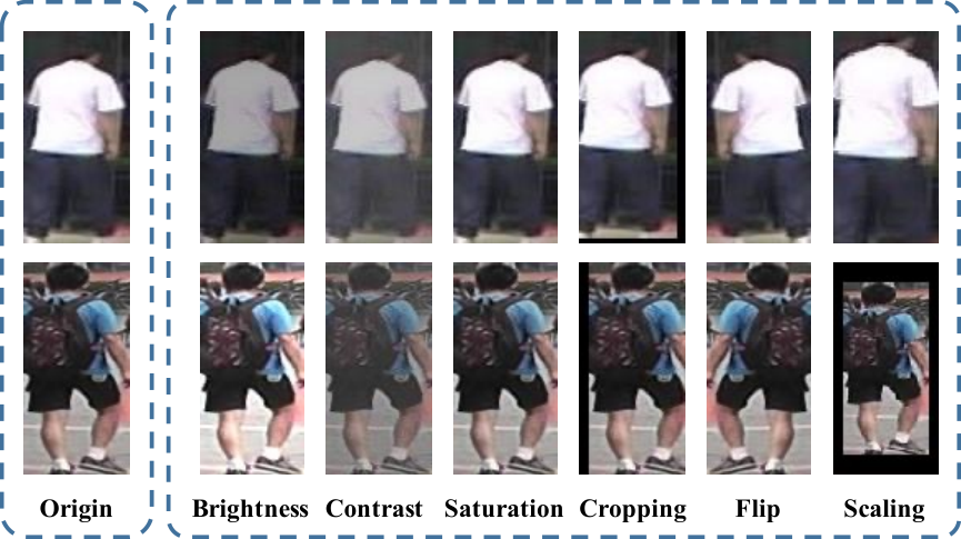
Table 11 shows an experiment on Market-1501 to analyze the feature invariance of pre-trained models. The original dataset is extended into six variations by applying six different augmentations to each image, to simulate some important appearance variances in the ReID task (examples shown in Figure 5). Then, Centered Kernel Alignment (CKA) cka scores can evaluate the similarity between the features of the origin dataset and the features of the each simulated dataset. The higher CKA score is, the features provided by the pre-trained model show better invariance on this type of augmentation. ViTI-S achieves the best CKA scores for all types of appearance variance, showing that ICS is beneficial for learning invariant features.
| Pre-train | Brig | Cont | Sat | Crop | Flip | Scale |
|---|---|---|---|---|---|---|
| ViTI-S | 0.809 | 0.818 | 0.998 | 0.927 | 0.996 | 0.820 |
| ViTC-S | 0.727 | 0.691 | 0.997 | 0.919 | 0.996 | 0.794 |
| ViT-S | 0.702 | 0.664 | 0.997 | 0.877 | 0.996 | 0.728 |
Appendix D Improvements of LUPerson Pre-training
| Pre-training | Market | MSMT17 | ||||
|---|---|---|---|---|---|---|
| Models | Data | Images | mAP | R1 | mAP | R1 |
| ViT-S | IMG-1K | 1.28M | 85.0 | 93.8 | 53.5 | 75.2 |
| LUP | 4.18M | 90.3 | 95.4 | 64.2 | 83.4 | |
| ViT-B | IMG-21K | 14.2M | 86.8 | 94.7 | 61.0 | 81.8 |
| LUP | 4.18M | 92.5 | 96.5 | 70.1 | 87.3 | |
Appendix E Theoretical Analysis of Generalization Performance
In this section, we give a theoretical analysis of generalization performance relating source and target data. In particular, we consider excess risk bound (ERB) as a measure of generalization performance, which is commonly used in the learning theory literature vapnik2013nature. The following informal theorem highlights the factors that influence the generalization of target task, which dramatically simplify Theorem 3.
Theorem 2 (Informal Version of Theorem 3).
Under the condition that the sample size of source data is larger than that of target data, then we have the following tow propositions to help improve generalization performance of target task:
- •
use the examples from the source data that close to target data;
- •
use a small learning rate to slightly update the backbone during the fine-tuning process.
In the remaining of this section, we first introduce the problem setting, and then present the formal theoretical result with its proof. To simplify the presentation of the proof, we include some supporting lemmas at the end of this section.
E.1 Problem Setting
To give an insight of the proposed method from the view of theoretical side, we formalize the problem as follows. We consider binary classification for simplicity. A domain is defined as a pair consisting of a distribution on inputs and a labeling function with . The labeling function can have a fractional (expected) value when labeling occurs non-deterministically. We denote by the source domain and the target domain. A hypothesis is a function , where is a hypothesis space on with VC dimension vapnik1971uniform . The loss on source domain that a hypothesis disagrees with a labeling function is defined as
| (10) |
where can also be a hypothesis. Its empirical version is written as
| (11) |
where is sampled from and is the sample size. Similarly, for target domain we define
| (12) | |||
| (13) |
where is sampled from and is the sample size.. Since the label function is deterministic for target task, the risk of a hypothesis is defined as
| (14) |
and the empirical risk is
| (15) |
Let define
The excess risk is defined by
| (16) |
which can be considered as a measure of generalization performance. Our goal is to minimize the excess risk.
For a hypothesis space , we give the definitions of the symmetric difference hypothesis space and its divergence following by ben2010theory.
Definition 3.
ben2010theory For a hypothesis space , the symmetric difference hypothesis space is the set of hypotheses forsome , where is the XOR function. That is, every hypothesis is the set of disagreements between two hypotheses in .
Definition 4.
ben2010theory For a hypothesis space , the -distance between two distributions and is defined as
Remark. The empirical version of -distance, denoted by , can be considered as the a measure of similarity between the sampled source data and the sampled target data .
E.2 Main Result and its Proof
Theorem 3 (Formal Version).
Let , finite samples of sizes , () drawn i.i.d. according , respectively. is the empirical -divergence between samples, then for any , with probability at least , we have
| (17) |
Remark. We make several comments of the ERB in Theorem 3. First, the bound shows that the unlabeled empirical -divergence (i.e., , the first term of the left hand side of bound (3)) is important to improve the generalization performance (reduce the excess risk), indicating that when the used source data and target data are close, it will have a good generalization performance in target task. Second, the bound needs the term is small for a hypothesis and the optimal hypothesis of source domain, which means that should be not too far from . This is consistent with the practice that usually a small learning rate is used to slightly update the backbone during the fine-tuning process. Finally, the term in the bound tells us that the source error obtained during the pre-training process is also important to the target performance.
Proof of Theorem 3.
By Lemma 1 we have
Here (a) uses Lemma 2 with the fact that since every can be represented as a linear threshold network of depth 2 with 2 hidden units, the VC dimension of is at most anthony1999neural; ben2010theory; (b) uses Hoeffding’s inequality in Lemma 3. Similarly, we have
∎
E.3 Supporting Lemmas
Lemma 1.
Define . For any , we have and
| (18) |
Proof.
By the definition of , we know this is symmetric. On the other hand, we have
∎
Lemma 2.
Let be a hypothesis space on with VC dimension . and be two distribution on and , finite samples of sizes , () drawn i.i.d. according , respectively. is the empirical H-divergence between samples, then for any , with probability at least , we have
| (19) |
Proof.
This lemma can be proved by a slight modification of Theorem 3.4 of kifer2004detecting. To this end, by setting and , then we know (since ) and
We then obtain (19) by using Theorem 3.4 of kifer2004detecting. ∎
Lemma 3 (Hoeffding’s inequality hoeffding1963probability).
Let be i.i.d. random variables with bounded intervals: , . Let , then we have