2021
Porous electrodes are an integral part of many electrochemical devices since they have high porosity to maximize electrochemical transport and high surface area to maximize activity. Traditional porous electrode materials are typically homogeneous, stochastic collections of small-scale particles and offer few opportunities to engineer higher performance. Fortunately, recent breakthroughs in advanced and additive manufacturing are yielding new methods to structure and pattern porous electrodes across length scales. These architected electrodes are emerging as a promising new technology to continue to drive improvement; however, it is still unclear which structures to employ and few tools are available to guide their design. In this work we address this gap by applying topology optimization to the design of porous electrodes. We demonstrate our framework on two applications: a porous electrode driving a steady Faradaic reaction and a transiently operated electrode in a supercapacitor. We present computationally designed electrodes that minimize energy losses in a half-cell. For low-conductivity materials, the optimization algorithm creates electrode designs with a hierarchy of length scales. Further, the designed electrodes are found to outperform undesigned, homogeneous electrodes. Finally, we present three-dimensional porous electrode designs. We thus establish a topology optimization framework for designing porous electrodes.
Topology optimization for the design of porous electrodes
keywords
Topology optimization, electrochemistry, electrochemical devices, porous electrodes, supercapacitors1 Introduction
Electrochemical devices are ubiquitous across society and play an increasingly critical role in addressing our global energy storage and conversion challenges. Beyond the more familiar applications like primary and secondary (rechargeable) batteries, these devices are enabling many of the novel, large-scale electrical energy storage (EES) technologies critical for driving the adoption of renewable electricity (Gür 2018). Large-scale integration is crucial, as renewable energies are the key for a sustainable and carbon-free future (Chu and Majumdar 2012; Chu et al 2016).
Secondary batteries, flow batteries, and supercapacitors can be employed to directly store and dispatch electrical energy and provide a buffer between the intermittency of electricity supply and demand (Gür 2018; Sawant et al 2021). Alternatively, electrochemical reactors and electrolyzers provide a pathway for converting electrical energy into chemical potential energy in the form of carbon and hydrogen fuels (Ager and Lapkin 2018; Stöckl et al 2021). In addition to providing a useful conduit for otherwise wasted excess electricity, for many of these reactors the feedstock is carbon dioxide, leading additionally to a reduction in greenhouse gases (O’Brien et al 2021; Lamaison et al 2021). More broadly, electrochemical devices employed as reactors are driving the electrification of industrial chemical manufacturing, further reducing or eliminating emissions (Schiffer and Manthiram 2017; Yan et al 2017; Shatskiy et al 2019; Stankiewicz and Nigar 2020; Barton 2020). Nevertheless, significant research, engineering and design effort is required to realize the benefits that these technologies offer, ensuring economic viability and guaranteeing widespread deployment (Chen et al 2018; Gür 2018).


Electrochemical devices include galvanic cells, which output energy, electrolytic cells, which require energy to perform a chemical transformation, and supercapacitors, which can dispatch energy through stored charge (Fuller and Harb 2018). Examples of galvanic cells include fuel cells and discharging batteries. Electrolytic cells include charging batteries, electrochemical reactors and electrolyzers. All of these devices share a common, core architecture typically composed of two porous electrodes immersed in an electrolyte and separated by a membrane or separator, as shown schematically in Figure 1.
The electrochemical processes driving performance occur at the electrode-electrolyte interface, and generally the higher the surface area, the higher the currents, power outputs, and energy storage. The porous electrode is often a coherent, stochastic collection of conductive micron-scale particles, and is principally engineered to yield the highest surface area per volume possible while minimizing electrical, fluid flow, and diffusive resistances as required by the specific application (Wang et al 2008; Weber et al 2011). The result is a monolith that can be characterized by a single porosity and single length scale for the constituent particles, leaving few opportunities for further engineering of the structure.
An emerging alternative to further increase electrochemical device performance is to employ architected electrodes (Forner-Cuenca and Brushett 2019; Park et al 2020; Zhang and Ran 2021). Instead of a simple, single-porosity monolith, the electrode can be composed of multiple materials, and shaped and patterned at multiple length scales. The concepts have been applied to generate high-performance, dual-scale lithium-ion batteries composed of energy-dense regions accessed by tailored, high-mobility channels (Bae et al 2013; Cobb and Blanco 2014; Nemani et al 2015; Zhang et al 2021). Similar ideas have also been used to improve redox flow battery performance (Zhou et al 2016). Spurred by advances in additive manufacturing and 3D printing (Ambrosi et al 2020), these efforts have been further extended to create patterned supercapacitors with superior energy density (Zhu et al 2016) and electrochemical flow reactors with improved productivity and mass transfer (Beck et al 2021a). These new manufacturing techniques are especially exciting, as they offer the promise of near arbitrary control over the porous electrode structure.
Advanced design tools are required to fully exploit these new manufacturing techniques and further improve electrochemical device performance. Topology optimization offers a novel opportunity to automatically design the multiscale, porous electrodes. The first application of these techniques focused on addressing design challenges in structural mechanics. In the pioneering work of Bendsøe 1989, the optimal design geometry was first formulated as a material distribution problem wherein a volume fraction field models the solid, void and intermediate material phases and incorporated the Solid Isotropic Material with Penalization (SIMP) method to penalize the intermediate phase and recover a discrete design. An alternative approach based on the level-set method (Wang et al 2003; Allaire et al 2002; Sethian and Wiegmann 2000) uses the zero isocontour of a level-set function to define the solid-void interface, thereby avoiding the intermediate phase.
Topology optimization techniques continue to be extended to more physically complex system including thermal, fluid, and coupled systems (Alexandersen and Andreasen 2020), but there have been limited applications of the ideas to electrochemical devices. Early work used level-set approaches to design electrodes for solid oxide fuel cells (Iwai et al 2011) and lithium-ion batteries (Zadin et al 2013). Topology optimization was also used to design a porous ionic-conducting scaffold for solid oxide fuel cell cathodes (Song et al 2013). More recent efforts have generally focused on the design of flow fields, which deliver fluids to porous electrodes, in the context of redox flow batteries (Yaji et al 2018; Chen et al 2019; Lin et al 2022) and fuel cells (Behrou et al 2019). While porous electrodes are part of these models, flow field architectures are the goal of the design problems. Other work on optimizing electrode structure has been limited to considering a smooth variation of the porosity field applied to the design of lithium-ion batteries (Ramadesigan et al 2010; Golmon et al 2012; Golmon et al 2014; Xue et al 2015) and redox flow batteries (Beck et al 2021b). In both cases, computational design and optimization lead to significant performance improvements over conventional, homogeneous-porosity electrodes. Performance improvements using graded porosity have also recently been experimentally demonstrated (Lu et al 2020). To the authors’ knowledge density-based topology optimization has not yet been applied to the design of the porous electrode itself, nor have these techniques been extended to transient and three-dimensional systems.

In this manuscript, we introduce the application of topology optimization to design porous electrodes for use in electrochemical devices. As shown in Figure 1, we separately consider the design of porous electrodes for steady-state and transient operation. Flow batteries, fuel cells and electrochemical reactors are ideally operated at steady-state and thus require constant fluid flow to supply and remove material, while batteries and supercapacitors transform material in situ and thus inherently operate transiently. We focus on simulation and optimization of the secondary current distribution, which provides a description of electrode performance when concentration polarization effects are unimportant (Haverkort 2019). In brief, the optimization algorithm is used to sculpt a porous material, here labeled ‘microporous’ to distinguish it from the larger pores generated by the optimization process and to emphasize the multiscale nature of the design, into an optimal architecture as shown in Figure 2.
In Section 2, we give a brief introduction of topology optimization applied to the design of porous electrodes. Then, in Section 3, we define the systems of partial differential equations (PDEs) for the ionic and electronic potentials describing the secondary current distribution in the porous electrodes. We then specialize these equations to describe model steady and transient applications, a porous electrode driving a reduction-oxidation Faradaic reaction (i.e., a ‘redox electrode’) and a charging supercapacitor, respectively. The equations are nondimensionalized in the context of seminal work on porous electrode theory to yield familiar dimensionless groups and provide generality (Newman and Tiedemann 1975). Implementation details and solution techniques are given in Section 4. Specifically, we include preconditioning techniques to accelerate the solution of the PDEs. In Section 5, we show various two-dimensional designs optimized for power efficiency, in the case of the redox electrode and for ohmic losses and stored energy in the supercapacitor electrode. We discuss the impact of the different dimensionless parameters and compare our designs with monolithic, homogeneous electrodes. Finally, we present examples of designed three-dimensional electrodes for each system.
2 Topology Optimization
The porous electrode design problem is to find the optimal distribution of material in a design domain , i.e.
| (1) | ||||
where is the cost function to be minimized and are the design constraints. The design variable defines the presence of a two porosity electrode ( for material with porosity and for material with porosity ). Note that this definition includes the extreme cases of the materials being pure electrolyte, , or pure solid, . The response functions and model the electronic and ionic potentials, respectively, according to the system of equations , whose details we explain in the next section.
In the context of density-based optimization Bendsøe 1989, the discrete nature of the design variable prevents using gradient-based algorithms. We therefore make the set of optimization variables convex by replacing with the continuous volume fraction variable . As explained in Section 3, the constitutive equations modeling the conductivities inherently penalize intermediate values of . We therefore do not use a penalization scheme such as SIMP (Bendsøe 1989).
Design problems in topology optimization are commonly ill-posed. Optimal designs consist of a non-converging sequence of highly oscillatory structures that maximize the surface area ad-infinitum. To obtain a well-posed problem, several techniques impose a minimum length scale in the design. Chief among them is the diffusion-reaction PDE filter (Lazarov and Sigmund 2011)
| (2) | |||||
where we solve for the filtered volume fraction given the design volume fraction . The filter radius controls the minimum length scale of the designs, denotes the boundary of , and , the outward pointing unit normal.
Since filtering inherently produces gray transition regions of intermediate material, projection of the filtered volume fraction to 0–1 values is often used to obtain sharper designs (Guest et al 2004; Wang et al 2011). However, continuation strategies are required to avoid convergence to low quality local minima. In this work, we obtain designs that are mostly discrete without projecting , so we leave out projection for simplicity. Future work could apply a projection method to obtain a sharper geometry.
3 Governing equations
In this section, we first describe a generic model that is applicable to most porous electrodes. We then apply it to the specific cases of a porous electrode driving a Faradaic reduction-oxidation reaction (i.e., a porous redox electrode) and a porous electrode used as an electrical double layer capacitor (EDLC) or supercapacitor.
Porous electrodes consist of a porous solid matrix of an electrically conductive material immersed in an electrolyte solution (c-f. Figure 2). Their modeling is determined by the conservation of the ionic and electronic current densities, on the assumption of constant concentration of chemical species and no charge separation (Newman and Tiedemann 1975). The current density transfer between the ionic and electronic current densities occurs at the interface, and it can be caused by either Faradaic, electrochemical reactions or charge storage at the Electrical Double Layer.
High-fidelity models of porous electrodes are computationally expensive due to their complex geometry and length scale disparity. Reduced-order models that capture essential quantities of interest without the costly modeling of the geometry are therefore desired. Most notably, the large-scale separation between the small pore structure (i.e., microporosity) and the electrode’s dimension permits the use of inexpensive models based on averaging techniques. These models resolve the potential fields at the electrode scale using effective material properties that capture the pore-scale effects (Newman and Tiedemann 1975; Newman and Thomas-Alyea 2012). Indeed, these effective properties are averages over representative elementary volumes containing both the solid matrix and the electrolyte phases. The Bruggeman correlation (Bruggeman 1935) is one such model in which the porosity and the tortuosity factor characterize the effective ionic conductivity
| (3) |
where is the conductivity of the electrolyte phase and the effective electronic conductivity
| (4) |
where is the conductivity of the solid phase. We remark here that the exponent penalizes the conductivity of intermediate densities as in SIMP (Bendsøe 1989). The current density transfer at the electrode-electrolyte interface is interpreted as an effective current per unit volume , where is the surface area of the interface between the microporous structure and the electrolyte per unit volume of the total electrode.
With the effective properties, we can model the porous electrode as a continuum, and we therefore solve for the electronic potential and ionic potential in the entire domain.
| in | (5a) | |||||
| in | (5b) | |||||
| on | (5c) | |||||
| on | (5d) | |||||
| on | (5e) | |||||
| on | (5f) | |||||
The domain boundary consists of two complementary regions for : , and over which, Dirichlet and homogeneous Neumann boundary conditions are applied, respectively. Similarly, is split for in and over which Robin and homogeneous Neumann boundary conditions are applied, respectively. The Robin boundary condition coefficients allows us to choose between applying only a potential, i.e. and , or only a current density and . We do not consider other options in this manuscript. These boundary conditions are for designing a porous electrode in a half-cell of an electrochemical device, where the membrane splitting the cell is the boundary (c-f. Figure 2). The domain is explicitly depicted in 2D and 3D in Figure 3. Design of the entire cell, i.e. with two electrodes, is left for future work. Finally, denotes the outward pointing unit normal.
We use the filtered design variable to parametrize the porosity
| (6) |
and the effective specific area per volume
| (7) |
where and are their specific area per volume for materials and , respectively. In this article, for simplicity, we consider and , i.e. a pure electrolyte phase for .
The Bruggeman correlation has been shown to overestimate the ionic conductivity for porous electrodes with different particle arrangement (Tjaden et al 2018; Tjaden et al 2016). Several researchers have proposed correction factors but there is still no consensus model (Koresh and Soffer 1977; Thorat et al 2009). In addition to the original Bruggeman correlation in (3), we thus consider a modification that results in lower effective ionic conductivity of the form , where takes values in the range depending on the electrode material (Madabattula and Kumar 2020). We penalize the electrode porosity in (6), so we do not affect the conductivity in the pure electrolyte phase, i.e. for :
| (8) |
where , and use it in (3) instead of (6), i.e.
| (9) |
3.1 Porous redox electrode
We consider the case of a porous electrode where a reduction-oxidation (redox) reaction occurs inside the porous electrode (Newman and Tiedemann 1975; Newman and Thomas-Alyea 2012). This is common in most porous electrodes operated at steady-state and constant concentration and often requires flowing electrolyte as shown in Figure 1(b). To distinguish this example we specify the model name as a “porous redox electrode.” Depending on the direction of the current and reaction term, this model could be used for devices such as discharging flow batteries, where a chemical reaction spontaneously generates current, or electrolyzers and charging batteries, where energy is inputted to activate the reaction.
The current generated due to the simple one electron transfer redox reaction , is described by the Butler-Volmer relationship (Fuller and Harb 2018)
| (10) |
where is the exchange current density, or just “exchange current,” corresponding to the reference concentration (Newman and Tiedemann 1975), and and are the concentration of reductant, , and oxidant, , respectively. The anodic and cathodic charge transfer (dimensionless) coefficients are and , respectively. For simplicity, we assume and . is the absolute temperature, is Faraday’s constant, and is the universal gas constant. Finally, is defined as the potential difference and is the standard potential for this reaction.
We supply the system with only an ionic current density
| (11) |
on , i.e. and in (5e), and ground the electronic potential at , cf. (5c). The rest of the boundary is electrically insulated, cf. (5d) and (5f). The total current supplied to the system, , is specified over the membrane area, . A positive current drives a chemical reaction and induces the porous redox electrode to act as an electrolyzer or charging battery.
Let be the thickness of the electrode, as illustrated in Figure 3. We replace the expressions (10), (11), and the nondimensional variables:
| (12) | ||||
| (13) | ||||
| (14) |
in the porous electrode system (5) to obtain the nondimensional equations of the porous redox electrode:
| in | (15a) | |||||
| in | (15b) | |||||
| on | (15c) | |||||
| on | (15d) | |||||
| on | (15e) | |||||
| on | (15f) | |||||
where
| (16) |
is the ratio of ohmic and kinetic resistances (it is an inverse Wagner number (Fuller and Harb 2018)),
| (17) |
is the ratio of liquid and solid conductivities and
| (18) |
is the dimensionless applied current density. Finally, the nondimensionalized Butler-Volmer term is
| (19) |
with . Note that in the linear regime of Butler-Volmer, cancels in the right-hand sides of (15a) and (15b).
3.2 Supercapacitor electrode
We also model a porous electrode operating under transient conditions. We again focus on a half-cell and specifically consider a single porous electrode of an EDLC, also commonly referred to as a supercapacitor (Fuller and Harb 2018). This serves as a model, transiently operated electrochemical device and can be extended to battery simulation. The latter involves added complexity in the governing equations, but the methodology for applying topology optimization to a transient electrochemical system is nevertheless well illustrated using an EDLC as a model. The supercapacitor behavior is governed by (5) and a time-dependent current transfer at the electrode-electrolyte interface
| (20) |
due to charge accumulation at the electrical double layer, where is the double layer capacitance (Newman and Tiedemann 1975).
We apply a charging current to the electrode by specifying a time-dependent ionic potential
| (21) |
on , i.e. and in (5e), and ground the electronic potential at , cf. (5c). The rest of the boundary is electrically insulated, cf. (5d) and (5f). The charging rate and the maximum potential modulate the input power and energy into the system. The timescales in the system are the characteristic charging time and the input charging time .
Replacing the expressions (20), (21) and the nondimensional variables
| (22) | ||||
| (23) | ||||
| (24) | ||||
| (25) |
in (5), we obtain the problem: Find and such that
| (26a) | ||||||
| (26b) | ||||||
| (26c) | ||||||
| (26d) | ||||||
| (26e) | ||||||
| (26f) | ||||||
for and as initial conditions. Only two nondimensional parameters determine and : as in (17), the ratio of electrolyte conductivity to electrode conductivities, and
| (27) |
the ratio of the characteristic time for charging to the total charging time.
4 Implementation
The two potential equations for both the porous redox electrode and the supercapacitor are solved using the finite element library Firedrake (Rathgeber et al 2016), which uses PETSc (Balay et al 2020) as the backend for the linear algebra. The sensitivities are automatically derived by pyadjoint (Mitusch et al 2019). The results of this paper can be reproduced using TOPE (Roy et al 2022). The MMA algorithm (Svanberg 1987) solves the optimization problems via the Python implementation pyMMAopt (Salazar de Troya 2021; Salazar de Troya et al 2021). We consider the optimized designs to have converged at three hundred iterations, as shown in Section 5.1.3.
Both problems are discretized using piecewise linear finite elements on triangular (2D) or tetrahedral (3D) meshes. The porous redox electrode problem is linearized using Newton’s method with an norm linesearch. The supercapacitor equation is integrated in time using a backward Euler scheme, and the cost function from (31), with a trapezoidal scheme. We integrate in time using 200 time steps for all simulations. An adaptive scheme is more efficient, but we leave it for future work. The calculation of sensitivities for large-scale transient problems can run into memory bottlenecks when using the adjoint method. Indeed, the method requires saving the entire state of the forward problem, i.e. the potentials at each time step, to calculate the adjoint variable. We did not encounter this problem, but future research with larger problems can use checkpointing schemes such as in Griewank and Walther 2000 or Zhang et al 2022 to overcome it.
For both the porous redox electrode and the supercapacitor, the linear system of equations resulting from the finite element discretization is of the form
| (28) |
where is the electronic potential coefficients, , the ionic potential coefficients, and and , their respective couplings. Correspondingly, we denote the electronic potential unknowns and residual by and , respectively, and the ionic potential unknowns and residual by and .
Instead of solving this linear system using a direct method, we consider a preconditioned iterative method (Wathen 2015) to improve scalability and solution time, especially for 3D simulations. The structure of the system enables preconditioning approaches where iterative methods are used for the different blocks.
First, the system (28) can easily be made symmetric for both the redox and supercapacitor problems by multiplying the ionic potential equations (15b) and (26b) by , respectively. Second, the diagonal blocks and result from the discretization of elliptic operators, making them ideal candidates for multigrid methods (Brandt 1977). We thus use the Conjugate Gradient method with a blockwise symmetric Gauss-Seidel preconditioner of the form
| (29) |
The diagonal blocks and are approximately inverted using a single AMG V-cycle (Ruge and Stüben 1987) (BoomerAMG (Henson and Yang 2002) from the hypre library (Falgout and Yang 2002)).
The PDE filter (2) is solved using a two-point flux approximation scheme described in Appendix B. For the linear system resulting from the discretization of the PDE filter, we use the Conjugate Gradient method preconditioned with an AMG V-cycle.
All PETSc solver options are given in Appendix C.
5 Optimal designs
We now present optimal designs for both the porous redox and supercapacitor/EDLC electrodes. The design domain in 2D and 3D, Figure 3(a) and Figure 3(b), respectively, receive the current or are subjected to an applied potential on and collect the current (ground the electronic potential) on . The computational domains are chosen such that the electrodes are twice as wide as they are thick and i.e. , while the membrane and current collector have lengths 75% of the electrode width, i.e. .
In 2D, we simulate half of the total domain with a mesh of approximately triangular elements and use the usual symmetry boundary conditions over the cut edges. We use a similar approach in 3D to only simulate a quarter of the domain with a mesh of approximately tetrahedral elements, and symmetry boundary conditions over the cut surfaces.
The first examples in both following subsections consider the original Bruggeman correlation in the effective ionic conductivity, cf. (3). The second set of examples uses the modified Bruggeman correlation in (8) with , which corresponds to the lowest factor in Madabattula and Kumar 2020. The filtered density is obtained using the PDE filter (2) with a filter radius of .
5.1 Porous redox electrode
We first design a porous redox electrode to minimize the ionic potential at the membrane for a fixed current density, i.e.
| (30) | ||||
which is equivalent to driving the overpotential to zero, defined as the excess necessary potential to drive the Faradaic reaction, . Regardless of the application, the most power efficient operation of this half-cell occurs when the cell operates as closely as possible to the thermodynamic potential. As evident in the expression, as , the potential difference in the half-cell approaches its thermodynamic limit. This minimization problem is thus equivalent to maximizing the power efficiency of the electrode.
Optimized designs are shown for various values of the conductivity ratio (17), the inverse Wagner number (16), and the dimensionless current density (18). The optimized designs start with an initial uniform everywhere in the domain.
Running on one core of an Intel Xeon E5-2695 v4 CPU, each optimization iteration (forward and adjoint problem) took between 0.9 to 1.5 seconds, depending on required the number of Newton iterations (1 to 5).
5.1.1 Original Bruggeman correlation
| 1 | 25 | ||
| 0.1 | |||
(a)

|
(b)

| ||
| 5 | |||
(c)

|
(d)

| ||
| 1 | 25 | ||
| 0.1 | |||
(a)

|
(b)

| ||
| 5 | |||
(c)

|
(d)

| ||
The optimized designs with the original Bruggeman correlation (3) in Figures 4 and 5 present a sharp teeth-like pattern. These teeth facilitate ionic transport since the effective ionic conductivity is higher in the electrolyte-only phase.
We note that for , the effective ionic conductivity (3) in the electrolyte-only phase () is greater than the effective electronic conductivity (4) in the porous phase () when . This implies that, with respect to reducing ohmic losses, the electrolyte-only phase is preferred over the porous phase when . Manifestly, reducing increases the proportion of the domain occupied by the porous phase. A further reduction of naturally results in a greater dominance of the porous phase.
On a similar note, increasing augments the relative importance of ohmic losses. Consequently, an increase in corresponds with a preference for the material with less ohmic resistance. For , this means an increase in electrolyte-only phase, and for , an increase in the porous phase.
The parameter also relates to electrode penetration depth (Fuller and Harb 2018). A small means that the reaction happens throughout the electrode, while a large means that the reaction happens closer to the membrane (or here closer to the electrolyte-only phase), due to increased ohmic resistance. In the absence of reactant consumption, a significant portion of the electrode is essentially unused for larger as observed in Figures 5 and 5. In that case, a thinner electrode would be more efficient, although here the electrode is forced to fill the domain to retain electrical contact.
The parameter represents the nondimensional current density at the membrane. In the linear regime of the Butler-Volmer equation (19), can be cancelled and is therefore assumed to have little effect over the optimal design. In the nonlinear regime, however, increasing it results in a greater reaction rate at a fixed potential difference in the electrode. Equivalently, at fixed currents the potential drop will be lower. We can investigate the nonlinearity of the Butler-Volmer equation by looking at the magnitude of in (19): a larger value, say greater than 2, indicates that we are in the nonlinear regime. For the chosen parameters, the cases with are in the linear regime, while for , the cases are slightly nonlinear and the cases are very nonlinear. It is clear that increasing increases the nonlinearity of . As for , reducing it leads to a decreased ohmic resistance. We thus observe larger potential differences and move further towards the nonlinear regime. As another indication of nonlinearity, we can look at the number of Newton iterations. The numbers of iterations required for solving the system for the initial design ( everywhere) are given in Table 1. We observe that increasing and decreasing increases the number of Newton iterations.
| 1 | 25 | |
| 0.1 | 2 | 1 |
| 5 | 5 | 3 |
| 1 | 25 |
| 2 | 1 |
| 4 | 2 |
In the cases, an increase in results in a slight increase in the electrolyte-only phase, the favored phase in terms of effective ionic conductivity. This increase is more pronounced for the case. On the other hand, there is little change for , especially for . Overall, the effect of is more significant for , where the Butler-Volmer is more nonlinear.
5.1.2 Modified Bruggeman correlation
| 1 | 25 | ||
| 0.1 | |||
(a)

|
(b)

| ||
| 5 | |||
(c)

|
(d)

| ||
| 1 | 25 | ||
| 0.1 | |||
(a)

|
(b)

| ||
| 5 | |||
(c)

|
(d)

| ||
Using the modified Bruggeman correlation (9), the designs in Figures 6 and 7 exhibit hierarchical root-like patterns, maintaining the teeth-like structure. The smaller, root-like channels or macropores facilitate ionic transport deeper inside the porous phase to compensate for the lower ionic conductivity. Interestingly, the optimization algorithm converged to a multiscale solution to improve the objective, corroborating experimental efforts suggesting this same strategy (Wang et al 2008).
Reducing has a different effect in this case. The effective ionic conductivity in the porous phase is less than of its value in the electrolyte-only phase. Reducing only favors the porous phase for , i.e. when ohmic resistance is higher. Additionally, a reduction of by a factor of 100 appears to increase the prevalence of root-like structures to facilitate ion transport.
As observed for the original Bruggeman correlation, an increase in corresponds with an increase in the phase that reduces ohmic losses, i.e. the electrolyte-only phase for , and the porous phase for .
Increasing also expands the electrolyte-only phase for , especially for due to the nonlinearity of Butler-Volmer as discussed in Section 5.1.1. However, there is little effect for smaller .
5.1.3 Convergence history

We briefly investigate the convergence of the optimization algorithm.
Considering the case with , , and the modified Bruggeman correlation, we plot the cost function evolution in Figure 8. The four insets in Figure 8 represent the evolution of the optimized design. We observe that most of the cost function reduction happens within the first 50 iterations. The design at 200 iterations is almost identical to the one obtained after 300 iterations as illustrated in Figure 7, a sign of convergence.
5.1.4 Comparison to a monolithic electrode
Original Bruggeman correlation


Modified Bruggeman correlation


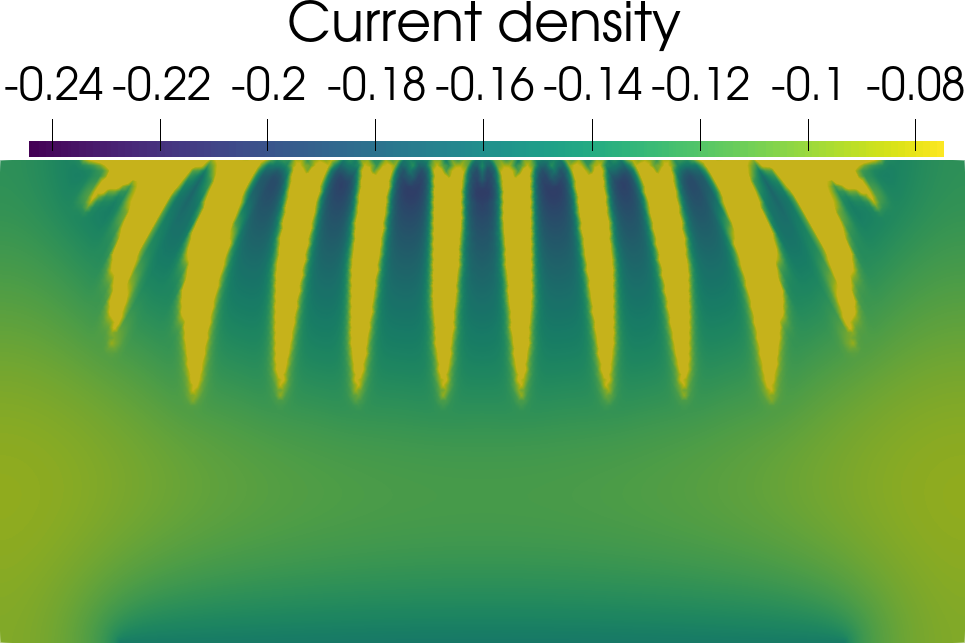
We compare the optimized electrodes to monolithic electrodes, i.e. an electrode consisting solely of the porous phase (). For each electrode, we plot the nondimensional ionic potential as well as the nondimensional volumetric charge transfer current density from (19), or current density for short.
In Figures 9(a)–9(b), we compare the design for and in Figure 4 to a monolithic electrode, both using the original Bruggeman correlation. We first observe that the distribution of the ionic potential is very similar, with only slightly higher potential values at the membrane for the monolithic electrode, corresponding to a slightly higher cost function . Indeed, the designed electrode leads to a 5.5% decrease in the average overpotential. The current density distribution is also similar, but appears more concentrated for the monolithic electrode. This indicates that spreading the reaction throughout the electrode is more efficient.
Now considering the modified Bruggeman correlation, we compare the designed electrode for and in Figure 7 to a monolithic electrode. Due to the very small effective ionic conductivity in the monolithic electrode, the ionic potential and current density are highly concentrated at the top boundary, cf. Figures 9(c)–9(d). In contrast, the ionic potential in the designed electrode spreads through the electrolyte-only channels, leading to a better distribution of the current density. This leads to an 84% reduction in the average overpotential. Again there is an apparent benefit to spreading the reaction across the electrode.
In brief, to reduce the overpotential, the optimizer favors designs that spread the current density throughout the electrode. When using the original Bruggeman correlation, teeth-like designs achieve this goal with a small increase in power efficiency. On the other hand, the modified correlation with lower effective ionic conductivity leads to root-like designs that are significantly more power efficient. This suggests that designing electrodes at multiple length scales is especially important in the case of lower effective ionic conductivity.
5.2 Supercapacitor electrode
We next pose the EDLC/supercapacitor electrode design problem as
| (31) | ||||
This minimizes the ohmic losses in the electrode, i.e. , subject to a constraint to ensure a minimum amount of stored energy, i.e. , at the end of the dimensionless charging time, . Equivalently, this minimizes the energy loss during the charge cycle of the system.
The stored energy is constrained to be greater than a factor of the maximum possible stored energy in the system
| (32) |
This corresponds to the domain being filled with porous material (i.e., and the domain is filled with only Material ) and the electrode being completely charged such that, at all points in the domain.
The penalization schemes for the nondimensional ionic conductivity
| (33) |
and the electronic conductivity
| (34) |
result in intermediate volume fraction values with higher current density than in (26). Similarly, these values have a lower contribution to the energy stored calculation due to the penalization . This strategy leaves intermediate values undesirable, and they are thus removed by the optimizer. An ultimate value of is desired for proper penalization. However, starting the optimization process with this value can cause convergence to unfavorable local minima. To circumvent this, a continuation strategy can be used: starting the optimizer with and changing to after 100 iterations. This continuation strategy leads to better optimized designs for the higher energy storage cases, but can create undesirable features for the lower energy storage cases. Therefore, we only use the continuation strategy for .
For the optimization study, we perform a parameter sweep on the conductivity ratio (17), the timescale ratio (27), and the constraint factor (31). The optimized designs start with an initial uniform everywhere in the domain, except the design in Figure 12 for which was used because it provided a better-connected design than . Running on one core of an Intel Xeon E5-2695 v4 CPU, each optimization iteration (forward and adjoint problem) took around 180 seconds.
5.2.1 Original Bruggeman correlation
| 0.05 | 0.005 | ||
| 0.1 | |||
(a)

|
(b)

| ||
| 0.01 | |||
(c)

|
(d)

| ||
| 0.05 | 0.005 | ||
| 0.1 | |||
(a)

|
(b)

| ||
| 0.01 | |||
(c)

|
(d)

| ||
The first set of optimized designs in Figures 10 and 11 uses the original Bruggeman correlation (3). The high ionic conductivity within the porous material () facilitates ion transport. As a consequence, the ions can penetrate deeper into the microporous network to access the high surface area within it, and thus the boundaries between the electrolyte and the porous material are generally smooth and have few protuberant, bulbous or jagged features to expose more of the microporous electrode. Additionally, the ion transport is efficient enough that the design is not substantially affected by lower charging times with respect to the ion transport timescale, i.e. higher . However, at lower , ionic current transport is less efficient with respect to electronic current transport. As such, the optimized designs have more mass closer to the top boundary, where the current enters the domain. Lastly, designs with higher energy stored requirements, cf. Figures 11, take more of the design domain to store more energy.
The cost function values of all optimized designs in Figures 10 and 11 show lower energy losses for lower values of (longer charging times). As expected, for the same maximum potential, longer charging times allow for a more gradual application of the potential field allowing the electrode to absorb the charge while minimizing irreversible, ohmic losses. In the limit of infinite charge times, the losses would further decay as the system approaches the reversible, thermodynamic limit. A higher energy constraint factor yields higher ohmic losses since currents are generally higher and more ions need to travel through the electrode. On the other hand, decreasing helps to alleviate these losses, especially for lower energy requirements and lower .
5.2.2 Modified Bruggeman correlation
| 0.05 | 0.005 | ||
| 0.1 | |||
(a)

|
(b)

| ||
| 0.01 | |||
(c)

|
(d)

| ||
| 0.05 | 0.005 | ||
| 0.1 | |||
(a)

|
(b)

| ||
| 0.01 | |||
(c)

|
(d)

| ||
The next set of examples uses the modified Bruggeman correlation for the effective ion conductivity, cf. (8). A lower effective ionic conductivity translates into worse ion transport within the electrode and lower ion penetration, forcing the design to increase the surface area exposed to the electrolyte to maximize the energy stored. As a result, and in contrast to the smooth designs described in the previous subsection, the optimization algorithm creates a hierarchical porous network with macropores for efficient ion transport, and smaller pores for greater energy storage, cf. the multi-lengthscale structure in Figures 12 and 13. This multiscale nature of the designs has been previously highlighted as an important route for attaining improved performance, and we emphasize that here the optimization algorithm automatically converged to a hierarchical design Wang et al 2008.
Varying does not noticeably affect the design for , cf Figure 12, but it does for , cf. Figure 13. The greater energy requirement for larger , i.e. faster charging times, requires more porous electrode to store more energy, at the cost of greater ohmic losses. The influence of the conductivity ratio is negligible for the nondimensional values tested here. Unlike for the original Bruggeman correlation, placing more porous electrode adjacent to the top boundary carries higher ohmic losses due to the lower ionic conductivity. Increasing the energy stored constraint factor did also translate into a growth of the electrode mass within the design domain.
The cost function values in Figures 12 and 13 follow a similar pattern to those in Figures 10 and 11 but with overall higher energy losses due to the reduced ionic conductivity. Importantly, the optimization algorithm again converged to a hierarchical structure to decrease energy loss and improve performance.
5.2.3 Comparison to a monolithic electrode


Our optimized designs for , and are now compared with a monolithic porous electrode, i.e. everywhere. We consider both the original and modified Bruggeman correlations and run simulations to compare the energy loss and the energy stored. We do not use the expressions in (31), i.e. and because they penalize intermediate volume fraction values, cf. (33), (34) in and in , and thus, do not reflect the real energy loss and energy stored. Instead, we express the energy loss as
| (35) | ||||
and the energy stored as
| (36) |
which are both derived from (26) and together they add up to the total energy inputted to the half-cell. For the designed electrode with the original Bruggeman correlation, is slightly lower than in Figure 11 and is slightly larger than 0.5 (). These differences are expected given the residual presence of the intermediate material, which overestimate the energy losses and underestimate the energy stored due to the penalization schemes.
The monolithic electrode simulations were performed for two different scenarios. First, the monolithic electrode was charged until the energy stored was equivalent to the energy stored in the designed electrode, and, second, the monolith was charged for the same amount of time for which the designed electrode was optimized.
| Fixed Energy Stored | Fixed Charging Time | Optimized Design | |
|---|---|---|---|
| 0.54947 | 0.96758 | 0.54947 | |
| 0.01655 | 0.02207 | 0.004196 | |
| Charging time factor | 0.755 | 1.0 | 1.0 |
| Fixed Energy Stored | Fixed Charging Time | Optimized Design | |
|---|---|---|---|
| 0.58426 | 0.34786 | 0.58426 | |
| 0.47853 | 0.32528 | 0.00419 | |
| Charging time factor | 1.21 | 1.0 | 1.0 |
When employing the original Bruggeman correlation, the designed electrode incurs 0.76% of the total energy input as ohmic losses, whereas the monolith incurs 2.9%, cf. Table 2. The designed electrode, however, is charged more slowly. Alternatively, when the monolithic electrode is charged for the same amount of time as the designed electrode, a larger amount of energy is stored, but 2.2% of the inputted energy is lost to ohmic heating, rendering the designed electrode more energy efficient. Figures 14(a), 14(c) and 14(e) compare the energy density field for the monolithic electrode operated at fixed charging time, fixed energy stored, and the optimized electrode. For these parameters the monolithic electrode charges evenly and shows a uniform stored energy density. For the designed electrode, the introduction of structure leads to non-uniform energy storage distribution but nevertheless leads to improved performance. The open channels lower the ohmic losses.
The impact of optimized structure is even more dramatic when using the modified Bruggeman correlation. Indeed, as seen in Table 3, the energy stored in the monolithic electrode charged for the same amount of time is only 60% of the optimized design while the ohmic losses are 48% of the input energy in the monolith and only 0.71% in the designed electrode. To attain the same amount of stored energy, the monolithic electrode incurs ohmic losses that are 114 times higher with a charging time 21% greater. As seen in Figure 14(b) and 14(d) the energy is accumulated mostly near the charging boundary because the ions cannot penetrate further into the monolithic electrode. On the other hand, the hierarchical structure of the optimized design facilitates ion transport to permit an efficient distribution of the energy density in the porous electrode, as observed in Figure 14(f).
5.3 Three-dimensional optimized designs


We further demonstrate the design of porous electrodes for the three-dimensional domain in Figure 3(b). Due to the computational cost of each three-dimensional simulation, we present a single optimized design for each problem.
First, we present a 3D optimized porous redox electrode in Figure 15(a), and its cross-section in Figure 15(b). For better contrast, the front slice of the cross-section is colored in black. To aid visualization on the unstructured grid, a smoothing filter is applied. We use the modified Bruggeman correlation and the parameter values , and . In 3D, a valley-like design is observed. Taking a cross-section reveals a root-like pattern similar to the 2D counterpart in Figure 6.
Next, we design a supercapacitor electrode using the parameters , and and the modified Bruggeman correlation as shown in Figure 15(c). In a similar fashion to the two-dimensional designs in Figure 13, the optimization algorithm creates a network with hierarchical porosity. Wide channels connect the top boundary to the bottom of the electrode and a series of more narrow channels that spring from them to increase the surface area. Most notably, a series of holes are carved on the exterior wall. The cross-section along the XY plane in Figure 15(d) resembles the designs in Figure 13.
6 Conclusion
In this work we have introduced the use of density-based topology optimization for the design of porous electrodes. We have demonstrated the generality of this approach by posing and solving optimization problems for two different electrochemical applications: a porous electrode driving a Faradaic reaction and an EDLC/supercapacitor electrode. These serve as model steady and transient systems, respectively. We presented the governing equations for the secondary current distribution of the two systems and identified the key nondimensional groups informing electrode design. The physical parameter inputs to the governing equations were interpolated using a design field representing two different microporous materials. This ensured an inherently multiscale design where the aim of the optimization problem was thus to pattern the two different materials at scales larger than their microporous lengthscale. The approach is general, but we set the porosity of one the microporous materials to 1, effectively modeling it as a pure electrolyte.
For both electrochemical examples, the topology optimization algorithm provides non-trivial optimized electrode designs. In all cases, the optimized design showed improved performance over an undesigned, monolithic single porosity electrode. This was additionally verified for two different Bruggeman correlations for the effective conductivity. For the porous redox electrode, this lead to overpotentials that were up to 84 % lower, while the supercapacitor electrode showed energy losses that were up to 98 % lower. All the designs showed that introducing new length scales improved performance, but the resultant designs corresponding to the modified Bruggeman correlation showed the emergence of hierarchical structures, consistent with recent literature (Liu et al 2017; Zhou et al 2016; Wu et al 2019; Cobb and Blanco 2014; Nemani et al 2015; Zhu et al 2016; Wang et al 2008). Finally, we further demonstrated the utility of these techniques by demonstrating three-dimensional electrode design, thus providing a potential pathway for manufacture and testing of high performance architected electrodes. This work thus provides a new design tool for the computational design of multiscale, architected porous electrodes.
Funding information
This work was performed under the auspices of the U.S. Department of Energy by Lawrence Livermore National Laboratory under Contract DE-AC52-07NA27344 and was supported by the LLNL-LDRD program under project numbers 19-ERD-035 and 20-ERD-019. LLNL Release Number LLNL-JRNL-828963.
References
- Ager and Lapkin (2018) Ager JW, Lapkin AA (2018) Chemical storage of renewable energy. Science 360(6390):707–708. 10.1126/science.aat7918
- Alexandersen and Andreasen (2020) Alexandersen J, Andreasen CS (2020) A review of topology optimisation for fluid-based problems. Fluids 5(1):29. 10.3390/fluids5010029
- Allaire et al (2002) Allaire G, Jouve F, Toader AM (2002) A level-set method for shape optimization. Comptes Rendus Mathématique 334(12):1125–1130. 10.1016/s1631-073x(02)02412-3
- Ambrosi et al (2020) Ambrosi A, Shi RRS, Webster RD (2020) 3D-printing for electrolytic processes and electrochemical flow systems. Journal of Materials Chemistry A 8(42):21,902–21,929. 10.1039/D0TA07939A
- Bae et al (2013) Bae CJ, Erdonmez CK, Halloran JW, et al (2013) Design of battery electrodes with dual-scale porosity to minimize tortuosity and maximize performance. Advanced Materials 25(9):1254–1258. 10.1002/adma.201204055
- Balay et al (2020) Balay S, Abhyankar S, Adams MF, et al (2020) PETSc users manual. Tech. Rep. ANL-95/11 - Revision 3.14, Argonne National Laboratory, URL https://www.mcs.anl.gov/petsc
- Barton (2020) Barton JL (2020) Electrification of the chemical industry. Science 368(6496):1181–1182. 10.1126/science.abb8061
- Beck et al (2021a) Beck VA, Ivanovskaya AN, Chandrasekaran S, et al (2021a) Inertially enhanced mass transport using 3D-printed porous flow-through electrodes with periodic lattice structures. Proceedings of the National Academy of Sciences 118(32):e2025562,118. 10.1073/pnas.2025562118
- Beck et al (2021b) Beck VA, Wong JJ, Jekel CF, et al (2021b) Computational design of microarchitected porous electrodes for redox flow batteries. Journal of Power Sources 512:230,453. 10.1016/j.jpowsour.2021.230453
- Behrou et al (2019) Behrou R, Pizzolato A, Forner-Cuenca A (2019) Topology optimization as a powerful tool to design advanced PEMFCs flow fields. International Journal of Heat and Mass Transfer 135:72–92. 10.1016/j.ijheatmasstransfer.2019.01.050
- Bendsøe (1989) Bendsøe MP (1989) Optimal shape design as a material distribution problem. Structural optimization 1(4):193–202. 10.1007/bf01650949
- Brandt (1977) Brandt A (1977) Multi-level adaptive solutions to boundary-value problems. Mathematics of Computation 31(138):333–390. 10.1090/s0025-5718-1977-0431719-x
- Bruggeman (1935) Bruggeman VD (1935) Berechnung verschiedener physikalischer konstanten von heterogenen substanzen. i. dielektrizitätskonstanten und leitfähigkeiten der mischkörper aus isotropen substanzen. Annalen der physik 416(7):636–664. 10.1002/andp.19374210205
- Chen et al (2018) Chen C, Kotyk JFK, Sheehan SW (2018) Progress toward commercial application of electrochemical carbon dioxide reduction. Chem 4(11):2571–2586. 10.1016/j.chempr.2018.08.019
- Chen et al (2019) Chen CH, Yaji K, Yamasaki S, et al (2019) Computational design of flow fields for vanadium redox flow batteries via topology optimization. Journal of Energy Storage 26:100,990. 10.1016/j.est.2019.100990
- Chu and Majumdar (2012) Chu S, Majumdar A (2012) Opportunities and challenges for a sustainable energy future. Nature 488(7411):294–303. 10.1038/nature11475
- Chu et al (2016) Chu S, Cui Y, Liu N (2016) The path towards sustainable energy. Nature Materials 16(1):16–22. 10.1038/nmat4834
- Cobb and Blanco (2014) Cobb CL, Blanco M (2014) Modeling mass and density distribution effects on the performance of co-extruded electrodes for high energy density lithium-ion batteries. Journal of Power Sources 249:357–366. 10.1016/j.jpowsour.2013.10.084
- Falgout and Yang (2002) Falgout RD, Yang UM (2002) hypre: A library of high performance preconditioners. In: International Conference on Computational Science, Springer, pp 632–641, 10.1007/3-540-47789-6_66
- Forner-Cuenca and Brushett (2019) Forner-Cuenca A, Brushett FR (2019) Engineering porous electrodes for next-generation redox flow batteries: recent progress and opportunities. Current Opinion in Electrochemistry 18:113–122. 10.1016/j.coelec.2019.11.002, publisher: Elsevier Ltd
- Fuller and Harb (2018) Fuller TF, Harb JN (2018) Electrochemical Engineering. John Wiley & Sons, Hoboken, NJ USA
- Geuzaine and Remacle (2009) Geuzaine C, Remacle JF (2009) Gmsh: A 3-D finite element mesh generator with built-in pre-and post-processing facilities. International journal for numerical methods in engineering 79(11):1309–1331. 10.1002/nme.2579
- Golmon et al (2012) Golmon S, Maute K, Dunn ML (2012) Multiscale design optimization of lithium ion batteries using adjoint sensitivity analysis. International Journal for Numerical Methods in Engineering 92(5):475–494. 10.1002/nme.4347
- Golmon et al (2014) Golmon S, Maute K, Dunn ML (2014) A design optimization methodology for Li+ batteries. Journal of Power Sources 253:239–250. 10.1016/j.jpowsour.2013.12.025
- Griewank and Walther (2000) Griewank A, Walther A (2000) Algorithm 799: Revolve: An implementation of checkpointing for the reverse or adjoint mode of computational differentiation. ACM Trans Math Softw 26(1):19–45. 10.1145/347837.347846
- Guest et al (2004) Guest JK, Prévost JH, Belytschko T (2004) Achieving minimum length scale in topology optimization using nodal design variables and projection functions. International journal for numerical methods in engineering 61(2):238–254. 10.1002/nme.1064
- Gür (2018) Gür TM (2018) Review of electrical energy storage technologies, materials and systems: challenges and prospects for large-scale grid storage. Energy & Environmental Science 11(10):2696–2767. 10.1039/c8ee01419a
- Haverkort (2019) Haverkort J (2019) A theoretical analysis of the optimal electrode thickness and porosity. Electrochimica Acta 295:846–860. 10.1016/j.electacta.2018.10.065
- Henson and Yang (2002) Henson VE, Yang UM (2002) BoomerAMG: A parallel algebraic multigrid solver and preconditioner. Applied Numerical Mathematics 41(1):155–177. 10.1016/s0168-9274(01)00115-5
- Iwai et al (2011) Iwai H, Kuroyanagi A, Saito M, et al (2011) Power generation enhancement of solid oxide fuel cell by cathode–electrolyte interface modification in mesoscale assisted by level set-based optimization calculation. Journal of Power Sources 196(7):3485–3495. 10.1016/j.jpowsour.2010.12.024
- Koresh and Soffer (1977) Koresh J, Soffer A (1977) Double layer capacitance and charging rate of ultramicroporous carbon electrodes. Journal of The Electrochemical Society 124(9):1379–1385. 10.1149/1.2133657
- Lamaison et al (2021) Lamaison S, Wakerley D, Kracke F, et al (2021) Designing a Zn–Ag catalyst matrix and electrolyzer system for conversion to CO and beyond. Adv Mater p 11. 10.1002/adma.202103963
- Lazarov and Sigmund (2011) Lazarov BS, Sigmund O (2011) Filters in topology optimization based on Helmholtz-type differential equations. International Journal for Numerical Methods in Engineering 86(6):765–781. 10.1002/nme.3072
- Lin et al (2022) Lin TY, Baker SE, Duoss EB, et al (2022) Topology optimization of 3d flow fields for flow batteries. arXiv preprint arXiv:220213032
- Liu et al (2017) Liu T, Zhang F, Song Y, et al (2017) Revitalizing carbon supercapacitor electrodes with hierarchical porous structures. Journal of Materials Chemistry A 5(34):17,705–17,733. 10.1039/c7ta05646j
- Lu et al (2020) Lu X, Bertei A, Finegan DP, et al (2020) 3D microstructure design of lithium-ion battery electrodes assisted by X-ray nano-computed tomography and modelling. Nature Communications 11(1). 10.1038/s41467-020-15811-x
- Madabattula and Kumar (2020) Madabattula G, Kumar S (2020) Model and measurement based insights into double layer capacitors: Voltage-dependent capacitance and low ionic conductivity in pores. Journal of The Electrochemical Society 167(8):080,535. 10.1149/1945-7111/ab90aa
- Mitusch et al (2019) Mitusch SK, Funke SW, Dokken JS (2019) dolfin-adjoint 2018.1: automated adjoints for FEniCS and Firedrake. Journal of Open Source Software 4(38):1292. 10.21105/joss.01292
- Nemani et al (2015) Nemani VP, Harris SJ, Smith KC (2015) Design of bi-tortuous, anisotropic graphite anodes for fast ion-transport in Li-ion batteries. Journal of The Electrochemical Society 162(8):A1415. 10.1149/ma2016-03/2/848
- Newman and Thomas-Alyea (2012) Newman J, Thomas-Alyea KE (2012) Electrochemical systems. John Wiley & Sons
- Newman and Tiedemann (1975) Newman J, Tiedemann W (1975) Porous-electrode theory with battery applications. AIChE Journal 21(1):25–41. 10.1002/aic.690210103
- O’Brien et al (2021) O’Brien CP, Miao RK, Liu S, et al (2021) Single pass conversion exceeding 85% in the electrosynthesis of multicarbon products via local regeneration. ACS Energy Letters 6(8):2952–2959. 10.1021/acsenergylett.1c01122
- Park et al (2020) Park SH, Goodall G, Kim WS (2020) Perspective on 3D-designed micro-supercapacitors. Materials & Design 193:108,797. 10.1016/j.matdes.2020.108797
- Ramadesigan et al (2010) Ramadesigan V, Methekar RN, Latinwo F, et al (2010) Optimal porosity distribution for minimized ohmic drop across a porous electrode. Journal of The Electrochemical Society 157(12):A1328. 10.1149/1.3495992
- Rathgeber et al (2016) Rathgeber F, Ham DA, Mitchell L, et al (2016) Firedrake: automating the finite element method by composing abstractions. ACM Transactions on Mathematical Software (TOMS) 43(3):1–27. 10.1145/2998441
- Roy et al (2022) Roy T, Salazar de Troya MA, Beck VA (2022) LLNL/TOPE: Topology optimization for porous electrodes. 10.5281/zenodo.6366849
- Ruge and Stüben (1987) Ruge JW, Stüben K (1987) Algebraic multigrid. In: Multigrid methods, vol 3 of Frontiers in Applied Mathematics. SIAM, Philadelphia, chap 4, p 73–130, 10.1137/1.9781611971057.ch4
- Sawant et al (2021) Sawant TV, Yim CS, Henry TJ, et al (2021) Harnessing interfacial electron transfer in redox flow batteries. Joule 5(2):360–378. 10.1016/j.joule.2020.11.022
- Schiffer and Manthiram (2017) Schiffer ZJ, Manthiram K (2017) Electrification and decarbonization of the chemical industry. Joule 1(1):10–14. 10.1016/j.joule.2017.07.008
- Sethian and Wiegmann (2000) Sethian J, Wiegmann A (2000) Structural boundary design via level set and immersed interface methods. Journal of Computational Physics 163(2):489 – 528. 10.1006/jcph.2000.6581
- Shatskiy et al (2019) Shatskiy A, Lundberg H, Kärkäs MD (2019) Organic electrosynthesis: Applications in complex molecule synthesis. ChemElectroChem 6(16):4067–4092. 10.1002/celc.201900435, publisher: John Wiley & Sons, Ltd
- Song et al (2013) Song X, Diaz A, Benard A, et al (2013) A 2D model for shape optimization of solid oxide fuel cell cathodes. Structural and Multidisciplinary Optimization 47(3):453–464. 10.1007/s00158-012-0837-x
- Stankiewicz and Nigar (2020) Stankiewicz AI, Nigar H (2020) Beyond electrolysis: old challenges and new concepts of electricity-driven chemical reactors. Reaction Chemistry & Engineering 5(6):1005–1016. 10.1039/D0RE00116C
- Stöckl et al (2021) Stöckl F, Schill WP, Zerrahn A (2021) Optimal supply chains and power sector benefits of green hydrogen. Scientific Reports 11(1):14,191. 10.1038/s41598-021-92511-6
- Svanberg (1987) Svanberg K (1987) The method of moving asymptotes – a new method for structural optimization. International journal for numerical methods in engineering 24(2):359–373. 10.1002/nme.1620240207
- Thorat et al (2009) Thorat IV, Stephenson DE, Zacharias NA, et al (2009) Quantifying tortuosity in porous Li-ion battery materials. Journal of Power Sources 188(2):592–600. 10.1016/j.jpowsour.2008.12.032
- Tjaden et al (2016) Tjaden B, Cooper SJ, Brett DJ, et al (2016) On the origin and application of the Bruggeman correlation for analysing transport phenomena in electrochemical systems. Current Opinion in Chemical Engineering 12:44–51. 10.1016/j.coche.2016.02.006
- Tjaden et al (2018) Tjaden B, Brett DJ, Shearing PR (2018) Tortuosity in electrochemical devices: a review of calculation approaches. International Materials Reviews 63(2):47–67. 10.1080/09506608.2016.1249995
- Salazar de Troya (2021) Salazar de Troya MA (2021) LLNL/pyMMAopt: Method of Moving Asymptotes for Firedrake. 10.5281/zenodo.5524961
- Salazar de Troya and Tortorelli (2020) Salazar de Troya MA, Tortorelli DA (2020) Three-dimensional adaptive mesh refinement in stress-constrained topology optimization. Structural and Multidisciplinary Optimization 62(5):2467–2479. 10.1007/s00158-020-02618-z
- Salazar de Troya et al (2021) Salazar de Troya MA, Oxberry GM, Petra CG, et al (2021) Another source of mesh dependence in topology optimization. arXiv preprint arXiv:210612098
- Wang et al (2008) Wang DW, Li F, Liu M, et al (2008) 3D aperiodic hierarchical porous graphitic carbon material for high-rate electrochemical capacitive energy storage. Angewandte Chemie International Edition 47(2):373–376. 10.1002/ange.200702721
- Wang et al (2011) Wang F, Lazarov BS, Sigmund O (2011) On projection methods, convergence and robust formulations in topology optimization. Structural and Multidisciplinary Optimization 43(6):767–784. 10.1007/s00158-010-0602-y
- Wang et al (2003) Wang MY, Wang X, Guo D (2003) A level set method for structural topology optimization. Computer methods in applied mechanics and engineering 192(1-2):227–246. 10.1016/s0045-7825(02)00559-5
- Wathen (2015) Wathen AJ (2015) Preconditioning. Acta Numerica 24:329–376. 10.1017/s0962492915000021
- Weber et al (2011) Weber AZ, Mench MM, Meyers JP, et al (2011) Redox flow batteries: a review. Journal of Applied Electrochemistry 41(10):1137–1164. 10.1007/s10800-011-0348-2
- Wu et al (2019) Wu Q, Lv Y, Lin L, et al (2019) An improved thin-film electrode for vanadium redox flow batteries enabled by a dual layered structure. Journal of Power Sources 410-411:152–161. 10.1016/j.jpowsour.2018.11.020
- Xue et al (2015) Xue N, Du W, Martins JR, et al (2015) Lithium-ion batteries: Thermomechanics, performance, and design optimization. In: Handbook of Clean Energy Systems, John Wiley & Sons Ltd., vol. 6. Wiley Online Library, p 2849–2864, 10.1002/9781118991978.hces225
- Yaji et al (2018) Yaji K, Yamasaki S, Tsushima S, et al (2018) Topology optimization for the design of flow fields in a redox flow battery. Structural and multidisciplinary optimization 57(2):535–546. 10.1007/s00158-017-1763-8
- Yan et al (2017) Yan M, Kawamata Y, Baran PS (2017) Synthetic organic electrochemical methods since 2000: On the verge of a renaissance. Chemical Reviews 117(21):13,230–13,319. 10.1021/acs.chemrev.7b00397
- Zadin et al (2013) Zadin V, Brandell D, Kasemägi H, et al (2013) Designing the 3D-microbattery geometry using the level-set method. Journal of power sources 244:417–428. 10.1016/j.jpowsour.2012.12.004
- Zhang et al (2022) Zhang H, Constantinescu EM, Smith BF (2022) PETSc TSAdjoint: a discrete adjoint ODE solver for first-order and second-order sensitivity analysis. SIAM Journal on Scientific Computing 44(1):C1–C24
- Zhang and Ran (2021) Zhang T, Ran F (2021) Design strategies of 3D carbon‐based electrodes for charge/ion transport in lithium ion battery and sodium ion battery. Advanced Functional Materials 31(17):2010,041. 10.1002/adfm.202010041
- Zhang et al (2021) Zhang X, Hui Z, King S, et al (2021) Tunable porous electrode architectures for enhanced Li-ion storage kinetics in thick electrodes. Nano Letters 21(13):5896–5904. 10.1021/acs.nanolett.1c02142
- Zhou et al (2016) Zhou X, Zeng Y, Zhu X, et al (2016) A high-performance dual-scale porous electrode for vanadium redox flow batteries. Journal of Power Sources 325:329–336. 10.1016/j.jpowsour.2016.06.048
- Zhu et al (2016) Zhu C, Liu T, Qian F, et al (2016) Supercapacitors based on three-dimensional hierarchical graphene aerogels with periodic macropores. Nano letters 16(6):3448–3456. 10.1021/acs.nanolett.5b04965
Appendix A Variational formulation
Here we provide the variational formulation of the system (5). It is necessary for the finite element method, which is used in our numerical experiments.
Let the bilinear forms
| (37) | ||||
the nonlinear mapping
| (38) |
and functional
| (39) |
Let the function spaces
| (40) | ||||
First, in the case where we have a Neumann boundary condition on , the variational formulation for (5) is given by: Find , such that
| (41) |
for all , Next, in the case where we have a Dirichlet boundary condition on , we require the additional function spaces
| (42) | ||||
The variational formulation for (5) is given by: Find , such that
| (43) |
for all , .
Appendix B Two-point flux approximation for the PDE filter
The PDE filter (2) is solved using a two-point flux approximation (TPFA) finite volume method that preserves the minimum principle: if for all , then attains its minimum on and . This principle is important to comply because negatives values of result in non-positive matrices and affect the iterative solver. Using Lagrange finite elements to discretize (2) does not ensure satisfaction of the minimum principle. Indeed, for a sufficiently small where is the mesh element size, the reaction term in (2) dominates the diffusion term. As such, effectively becomes the -orthogonal projection of onto , which necessitates oscillations to minimize the -distance (Salazar de Troya and Tortorelli 2020).
Given a partition on , let denote the union of all interior facets. We define the jump at a facet by , where and are the limit values of on either side of the facet. Let be the piecewise constant function of cell-centered coordinates. Let be the space of piecewise constant functions on our partition of . The variational problem is given by: Find such that
| (44) |
for all .
It is known that in order for TPFA to converge, the jump of the cell centers must be orthogonal to the facet between the cells. This is not in general satisfied by unstructured meshes. We employ the Frontal-Delaunay algorithm in Gmsh (Geuzaine and Remacle 2009) that ensures most of the mesh elements are equilateral triangles/tetrahedra and therefore, their centroids are connected with lines orthogonal to the facets. One could also instead use a mixed formulation where piecewise constant elements are used for and lowest-order Raviart-Thomas elements are used for the flux .
Appendix C PETSc solver options
For the redox electrode, the PETSc nonlinear solver options are:
The preconditioner (29) is specially suited for block preconditioning using Firedrake’s solver interface with PETSc. The solver options are given by:
We use the following PETSc solver options for the PDE filter: