In our model we describe particles constrained to a spherical surface and interacting via a two-body, isotropic potential $v(r)$ given by a hard core followed by a short-range attractive and long-range repulsive (SALR) tail $w(r)$, with $r$ being the euclidean distance, which we model as the sum of two Yukawa functions of opposite signs:

$$v(r)=\begin{cases}\displaystyle{\infty},&\text{if}\ r<\sigma^{*}\\ -\displaystyle{\frac{R\varepsilon}{r}}\bigg[\exp\big(-\gamma_{1}r/\sigma^{*}\big)-A\exp\big(-\gamma_{2}r/\sigma^{*}\big)\bigg],&\text{otherwise}\end{cases}$$

(1)

This definition introduces four different lengthscales: $R$ is the radius of the sphere; the diameter $\sigma^{*}=R\sqrt{2-2\cos\frac{\sigma}{R}}$ is defined in terms of the curvilinear diameter $\sigma$, i.e. the minimum geodesic distance two particles can achieve without overlapping; $\gamma_{1}/\sigma^{*}$ and $\gamma_{2}/\sigma^{*}$ are the inverse of the attractive and repulsive ranges respectively. We will measure lengths in units of $R$ and set $\gamma_{1}=\frac{5}{6}$ and $\gamma_{2}=\frac{1}{2}\gamma_{1}$, so that we only need to specify one lengthscale, namely $\sigma$.

The other quantities which define the potential are the attractive amplitude $\varepsilon$, which we set to $1$, and the repulsive amplitude $A$. Here we follow a previous work ³: we choose $A$ so that $\int\mathrm{d}\hat{x}\,w(\hat{x})=0$. In order to do so, we adopt the standard prescription of fixing the tail inside the hard-core region to its minimum, $w(\sigma^{*})$. This gives us the following expression for the amplitude:

$$A=\frac{1}{2}\frac{\big(\gamma_{1}+2\big)e^{-\gamma_{1}}-2e^{-2R\gamma_{2}/\sigma^{*}}}{\big(\gamma_{2}+2\big)e^{-\gamma_{2}}-2e^{-2R\gamma_{1}/\sigma^{*}}},$$

(2)

which gives $A\simeq 0.3866$ at $\sigma/R=0.1$ for the values of $\gamma_{1}$ and $\gamma_{2}$ used here.

Examples of the potential can be seen in figure 1, where we also plot the spherical harmonics coefficients of the SALR tail, defined by:

$$w_{\ell}=\int\mathrm{d}\hat{x}\,w(\hat{x})\mathrm{Y}_{\ell,0}(\hat{x}),$$

(3)

where $\hat{x}$ represents the coordinates of a point on the surface of a unitary sphere. Notice we only need to retrieve the $m=0$ components using the zonal spherical harmonics $Y_{\ell,0}(\hat{x})$, thanks to the rotational symmetry of the potential. Moreover we consider real spherical harmonics, since all the functions we consider are real. These coefficients display negative minima at $\ell^{*}=6$ and $\ell^{*}=3$ respectively for $\sigma/R=0.1$ and $\sigma/R=0.2$: we will show in the next section that this property leads to the formation of microphases.

We also introduce here the other quantities which we are going to use throughout the paper. The density of $N$ particles on the sphere is given by $\rho=N/(4\pi R^{2})$. For simplicity we shall use the adimensional quantity $\rho R^{2}$. Since the particles have a finite size $\sigma$ we also introduce the packing fraction $\eta$ which is the ratio between the total surface area of the sphere and the area occupied by the particles. Using the equation for the area of a spherical cap of curvilinear diameter $\sigma$ we obtain $\eta=2\pi R^{2}(1-\cos\frac{\sigma}{2R})\rho$. Notice that while in principle $\eta$ can vary between $0$ and $1$, the actual upper limit is given by the close packing fraction of the disks, which on a plane would be achieved by the hexagonal lattice packing $\eta_{CP}=\frac{\pi\sqrt{3}}{6}\sim 0.9069$. The problem of finding the optimal packing of $N$ disks on a spherical surface is still open, but since we will consider small $\sigma/R$ ratios we can consider the planar close packing as an appropriate approximate upper boundary for the packing fraction $\eta$. We measure the temperature of the system in reduced units $T^{*}=k_{B}T/\epsilon$, where $k_{B}$ is the Boltzmann constant. Notice that some of the attractive effective interactions that may lead to the SALR potential can be described by athermal phenomena (such as depletion), so the inverse temperature $\beta=\epsilon/k_{B}T$ can also be interpreted as a concentration of depletants. Finally, since we will work in the grand canonical ensemble, we also introduce the chemical potential $\mu$.

The SALR potential is well known to form clusters and other inhomogeneous phases ³⁹. The attractive part of the potential helps particles aggregate when the density of the fluid is large enough, however the repulsive tail keeps the size of the agglomerates finite, leading to a complex behavior in which particles arrange in a variety of different patterns depending on the thermodynamic state of the system.

In the next section we will build the tools needed to make this qualitative argument for the emergence of inhomogeneous phases in SALR fluids more quantitative and obtain a phase diagram of the system, similarly to what was done for soft-core fluids on a sphere ²⁵.

To describe this system we use a density functional theory (DFT), which expresses the grand potential $\beta\Omega$ of the fluid as a functional of its density profile $\rho(\hat{x})$. For interacting systems the exact functional is generally unknown, so we resort to an approximation where a simple mean field perturbation is applied to a reference functional which contains the ideal gas and the hard-core contributions. The former is known exactly, but the latter must again be obtained from some sort of approximation. A local density approximation (LDA) for the free energy of a fluid of hard disks can be obtained from equation of states known in the literature, which in turn have been derived by a variety of tools such as virial expansion and integral equations. Here we follow Archer ⁹ in using the scaled-particle approximation. This gives us the following grand potential functional defined on the unit sphere $S^{2}$

	$\displaystyle\beta\Omega[\rho]=\beta\mathscr{F}_{id}+\beta\mathscr{F}_{HD}+\beta\mathscr{F}_{P}+\beta\mathscr{F}_{ext}-\beta\mu N$		(4)
	$\displaystyle\beta\mathscr{F}_{id}-\beta\mu N=\int_{S^{2}}\mathrm{d}\hat{x}\,\rho(\hat{x})\big[\ln(\rho(\hat{x})\delta_{TH}^{2})-1-\beta\mu\big]$
	$\displaystyle\beta\mathscr{F}_{HD}=\int_{S^{2}}\mathrm{d}\hat{x}\,\rho(\hat{x})\big[(1-\eta(\hat{x}))^{-1}-\ln(1-\eta(\hat{x}))-1\big]$
	$\displaystyle\beta\mathscr{F}_{P}=\frac{1}{2}\beta\int_{S^{2}}\int_{S^{2}}\mathrm{d}\hat{x}\mathrm{d}\hat{x}^{\prime}\,\rho(\hat{x})\rho(\hat{x}^{\prime})w(\hat{x},\hat{x}^{\prime})$
	$\displaystyle\beta\mathscr{F}_{ex}=\beta\int_{S^{2}}\mathrm{d}\hat{x}\,\rho(\hat{x})\phi(\hat{x})$

where $\mathscr{F}_{id}$ is the ideal-gas free energy, $\mathscr{F}_{HD}$ is the hard-disk contribution, $\mathscr{F}_{ext}$ is the contribution due to the action of an external field $\phi$ and $\mathscr{F}_{P}$ is the excess free energy due to the contribution of the interaction potential. We have also introduced the thermal length $\delta_{TH}=\sqrt{\frac{h^{2}\beta}{2\pi m}}$, $h$ being the Planck constant and $m$ being the mass of a particle.

It should be noted that the functional we employ is quite crude with respect to more accurate functionals available in the literature, both for the hard-disk contribution and for the excess free energy term. For example, fundamental measure theory provides reference functionals for the hard-disk contributions that can accurately probe the fluctuations of the density profile even on the lengthscale of the disk diameter ²⁶, while the LDA functional used here will only provide useful information about the profile on the much larger lengthscale of the meso-structures found in the system ⁹. Moreover we derive the reference functional from an equation of state which is valid for a planar system, and one may be concerned that a spherical system would require corrections to this equation of state and hence to the functional: however numerical solutions of the Percus-Yevic equation for hard-disks on a sphere surface ²⁷ show that the correction is of second order on $\sigma/R$ and does not have a large impact for the relatively small values of this parameter considered here.

On the other hand, the excess free energy due to the non singular part of the potential which we use is known to be inaccurate when describing the critical point of the phase diagram, because it is the result of a mean field approximation. This inaccuracy was brought forth in a simulation study of a three-dimensional SALR fluid in the bulk ²⁸, which showed that the phase portrait is qualitatively different from the mean-field picture, especially as the high-temperature limit of the inhomogeneous phases is reached, and thermal fluctuations become important. In fact, both approaches predict the same kind of periodic structures, namely, cluster, tubular and lamellar phases in order of increasing density. However, according to the mean-field DFT all of the above phases survive up to the highest temperature at which the system is inhomogeneous, whereas in the simulation, as the temperature increases, the cluster phase melts first, to be followed by the tubular phase, and finally by the lamellae. Moreover, the whole inhomogeneous domain is shifted to higher densities compared to the mean-field DFT predictions.

The fact that these discrepancies should be traced back to the mean-field approximation was made clear in a subsequent theoretical investigation ²⁹, in which fluctuations are taken into account on the top of the mean-field result, and the phase diagram thus obtained displays the same qualitative features obtained in the simulations.

All the above concerns are well funded, but here we opt for simplicity, even though this may affect the accuracy of our findings. We will not be able to describe the internal structure of clusters and other meso-structures, and we will not obtain an accurate description of the critical point in the phase diagram using this functional. Nevertheless we will be able to compute a qualitative phase diagram of the system. We will also be able to compare our results for the homogeneous fluid to simulations we performed.

Once we have a functional, we can obtain the equilibrium density profile by solving the Euler-Lagrange equations in search of a global minimum of the thermodynamic potential:

$\displaystyle\frac{\delta\beta\Omega[\rho]}{\delta\rho(\hat{x})}=0.$

(5)

In general these equations do not have a single solution for a given thermodynamic state, meaning that the system has different metastable states, so one needs to obtain the profiles of different minima and compare their grand potentials. Moreover these equations are not usually analytically solvable, so the results are obtained through numerical methods ³⁰³²⁵.

The homogeneous fluid is a special case in which one can obtain an analytical solution by plugging in the equations a flat density profile. Using a homogeneous density does not always lead to a stable solution, that is, the homogeneous fluid may not be a local minimum of the grand potential. However one can always recast the functional in terms of the density of the homogeneous solution $\bar{\rho}$ and its packing fraction $\bar{\eta}$, instead of the chemical potential $\mu$. From the homogeneous solution of the Euler-Lagrange equations we obtain

	$\displaystyle\beta\mu=\ln(\bar{\rho}\delta_{TH}^{2})+\beta\mu^{ex},$		(6)
	$\displaystyle\beta\mu^{ex}\equiv\frac{3\bar{\eta}-2\bar{\eta}^{2}}{(1-\bar{\eta})^{2}}-\ln(1-\bar{\eta})+\int_{S^{2}}\mathrm{d}\hat{x}\,w(\hat{x}),$

where we have introduced the excess chemical potential $\mu^{ex}$, which allows us to rewrite the ideal gas reference functional as

$$\beta\mathscr{F}_{id}-\beta\mu N=\int_{S^{2}}\mathrm{d}\hat{x}\,\rho(\hat{x})\big[\ln(\rho(\hat{x})/\bar{\rho})-1-\beta\mu^{ex}\big].$$

(7)

Since we will study the phase diagram in terms of the density $\rho$ of the fluid, rather than its chemical potential $\mu$, this parametrization of $\mu^{ex}$ will simplify the task of exploring the thermodynamic states of the system, by allowing us to obtain an approximate location of each sampled thermodynamic state on the phase diagram.

In order to solve the Euler-Lagrange equations we adapt the minimization algorithm previously developed for bulk ³ and spherical systems ²⁵ of soft particles, which uses the SHTOOLS python module to compute spherical harmonics ^{31, 32} . This algorithm discretizes the density profile over a $K\times 2K$ grid of equispaced points in $\theta$ and $\phi$, and proceeds to minimize the grand potential of the discretized density profile using an optimized version of the gradient descent algorithm. In this way we allow the algorithm to freely explore virtually any density profile, instead of limiting ourselves to a set of profiles obtained a priori. This is especially useful because the sphere topology prevents the formation of perfect lattices and the positions of the disclinations defects can be difficult to guess a priori. Moreover, it lets us explore unexpected metastable patterns, such as spiral phases, which would be discarded otherwise. The trade off is that the algorithm still needs a set of initial density profiles from which to start the gradient descent, which must be chosen so as to explore as much of the free energy landscape as possible. We employ different starting conditions using (i) random patterns, (ii) striped patterns, (iii) high density spots at the vertices of regular polyhedra, (iv) low density spots at the vertices of regular polyhedra, (v) profiles obtained from previous runs of the minimization algorithm. Even with this setup, it must be noted that there is no absolute guarantee that the final density profile is truly the global minimum. However by comparing our results with previous ones we can achieve a good degree of confidence in their overall correctness. We set the parameter $K$ determining the number of grid points at $K=256$. For this choice of $K$, the algorithm is still rapidly convergent, as shown in figure S3 of the Supporting Material, while at the same time its results are basically unaffected by the discretization. In fact, halving or doubling $K$ does not lead to appreciable changes in the grand potential at convergence, as displayed in figure S4 of the Supporting Material. Moreover, we show in figures S5, S6, and S7 of the Supporting Material that the equilibrium distribution at three different densities is also unaffected by halving or doubling $K$.

We still need to show that the system allows the formation of equilibrium inhomogeneous patterns. To do so, consider the functional we have described: the trivial homogeneous solution to the Euler-Lagrange equations is not necessarily a minimum of the grand potential. For this to be the case, it must satisfy the additional condition that the density profile $\bar{\rho}$ is stable with respect to arbitrary small fluctuations $\delta\rho(\hat{x})$

$$\int_{S^{2}}\int_{S^{2}}\mathrm{d}\hat{x}\mathrm{d}\hat{x}^{\prime}\,\delta\rho(\hat{x})\delta\rho(\hat{x}^{\prime})c(\hat{x},\hat{x}^{\prime})<0\,,$$

(8)

where we introduced the direct correlation function $c(\hat{x},\hat{x}^{\prime})$ given by

$$c(\hat{x},\hat{x}^{\prime})\equiv-\frac{\delta\beta\Omega}{\delta\rho(\hat{x})\delta\rho(\hat{x}^{\prime})}\bigg|_{\bar{\rho}}.$$

(9)

We remark that the above definition also contains the ideal gas contribution to $c(\hat{x},\hat{x}^{\prime})$. For a homogeneous fluid, the direct correlation function is isotropic, so $c(\hat{x},\hat{x}^{\prime})\equiv c(\cos\theta)$, where $\theta=\arccos{(\hat{x}\cdot\hat{x}^{\prime})}$, and we can write it as a spherical harmonics series

	$\displaystyle c(\cos\theta)=\sum_{\ell}c_{\ell}\mathrm{Y}_{\ell,0}(\cos\theta)$		(10)
	$\displaystyle c_{\ell}=\int_{S^{2}}\mathrm{d}\hat{x}\,c(\cos\theta)\mathrm{Y}_{\ell,0}(\cos\theta).$

We can then use the spherical convolution theorem to rewrite the condition (8) as

$$\sum_{\ell,m}\sqrt{\frac{4\pi}{2\ell+1}}c_{\ell}(\delta\rho)_{\ell,m}^{2}<0$$

(11)

which, thanks to the fact that fluctuations $\delta\rho(\hat{x})$ can be chosen arbitrarily, becomes $\sqrt{\frac{4\pi}{2\ell+1}}c_{\ell}<0$ for any $\ell$. Finally we can compute these coefficients explicitly to obtain

$$\sqrt{\frac{4\pi}{2\ell+1}}c_{\ell}=-\frac{1+\bar{\eta}}{\bar{\rho}(1-\bar{\eta})^{3}}-\beta\sqrt{\frac{4\pi}{2\ell+1}}w_{\ell}<0.$$

(12)

If the non singular part of the interaction potential has any negative harmonic coefficients $w_{\ell}$, one can find some thermodynamic state for which the condition is not satisfied at least for some harmonic degree $\ell$ ^{33, 25}. Then there will be a negative minimum of the coefficients $w_{\ell}$ at some harmonic order $\ell^{*}$ which defines the largest region in the phase diagram in which the homogeneous solution is unstable. This region will then necessarily be populated by some inhomogeneous phases which are stable solutions of eq. (5), so that the existence of a negative minimum $w_{\ell^{*}}$ in the harmonic coefficients of the potential becomes the criterion for microphase separation to be possible. The boundary of this instability region is defined by

$$\frac{1+\bar{\eta}}{\bar{\rho}(1-\bar{\eta})^{3}}=-\beta{\sqrt{\frac{4\pi}{2\ell^{*}}+1}}w_{\ell^{*}},$$

(13)

and it takes the name of $\lambda$-line ³⁴. Notice that while stability is a necessary condition for a phase to be the equilibrium state of the system, it is not a sufficient condition: this means that, while the homogeneous fluid is stable at temperatures above that of the $\lambda$-line for the $\bar{\rho}$ at hand, it is not necessarily the equilibrium solution.

As shown in the inset of figure 1, $w_{\ell}$ does indeed display a negative minimum at $\ell^{*}=6$ for $\sigma/R=0.1$ and at $\ell^{*}=3$ for $\sigma/R=0.2$, which means the phase diagram of the SALR system contains inhomogeneous phases.

In order to test the reliability of our mean field approximation, we will use Monte Carlo (MC) simulations of the SALR model in the canonical ensemble, that is at fixed number of particles $N$, surface area $A$, and temperature $T$, following the same framework we used for the GEM4 fluid ²⁵.

The moves of the MC are rotations of a particle around a random axis orthogonal to its position vector. More specifically we consider a particles of coordinates $\hat{x}=[\cos\phi\sin\theta,\sin\phi\sin\theta,\cos\theta]$ and use its position as the north pole of a new coordinate system, so that its new coordinates are $\hat{x}_{0}=[0,0,1]$. Then, we randomly choose a new value $\cos\theta^{\prime}$ for its third component $z$ in the interval $[1,1-\delta]$ (setting the maximum stride of the particle to $\delta=0.4R$), and choose a direction for the move $\phi^{\prime}\in[0,2\pi]$. The new position in the new coordinate system is given by $\hat{x}_{0}^{\prime}=[\cos\phi^{\prime}\sin\theta^{\prime},\sin\phi^{\prime}\sin\theta^{\prime},\cos\theta^{\prime}]$. Finally we return to the original coordinate system by applying the rotation that satisfies $\hat{R}\hat{x}_{0}=\hat{x}$, so that we obtain the new coordinates as $\hat{x}^{\prime}=\hat{R}\hat{x}_{0}^{\prime}$.

Contrary to the GEM4 model and other soft-core fluids, the presence of a hard-core in SALR model presents the additional challenge of avoiding metastable configurations in which particles can easily get stuck: obtaining a faithful representation of the inhomogeneous phases through simulations at high density can be difficult and goes beyond the scope of this paper. Hence our simulations will only focus on the homogeneous fluid in the low density regime. This requires using a low number of particles, so we only sample the interval $N\in[2,150]$.

Each sampled trajectory contains $500\,000$ steps, but the first $150\,000$ steps are discarded when computing the correlation functions, in order to allow the system to thermalize.

Before we consider the full phase diagram, we can characterize the homogeneous fluid. As discussed in the previous section, in this regime correlation functions are isotropic and can be computed directly from the functional. Once one has computed the direct correlation function $c(\hat{x},\hat{x}^{\prime})$, the total correlation function $h(\hat{x},\hat{x}^{\prime})$ can be obtained by solving the Ornstein-Zernike equation ^{35, 36} for the spherical harmonics coefficients

$$h_{\ell}=\frac{c_{\ell}}{1-\rho\sqrt{\frac{4\pi}{2\ell+1}}c_{\ell}},$$

(14)

from which one can then compute both the radial distribution function $g(r)=1+h(r)$ and the structure factor

$$\sqrt{\frac{4\pi}{2\ell+1}}S_{\ell}=1+\rho\sqrt{\frac{4\pi}{2\ell+1}}h_{\ell}.$$

(15)

However this is not the most accurate path to correlation functions, because the LDA reference functional for hard disks gives a direct correlation function proportional to $\delta(\hat{x},\hat{x}^{\prime})$, so that in (12) the hard disk contribution has no dependence on the harmonic order $\ell$. An alternative route to correlations is using the Percus test-particle method ³⁷: using the functional defined in (4), we consider the action of a single particle fixed at the north pole of the sphere on the rest of the fluid, that is, we set $\phi(\hat{x})=v(\hat{x})$. Then the equilibrium distribution for states above of the $\lambda$-line is proportional to the radial distribution function $g(r)=\rho(\hat{x})/\rho$, and from this definition one can easily obtain the structure factor $S_{\ell}$ using the previous relations.

In figure 2 we show an example of the radial distribution function obtained at $T^{*}=1$, $\sigma/R=0.1$ and $N=75$, comparing theory and simulation. Theory is able to describe the first shell of neighboring particles (the peak at $r/\sigma^{*}=1$) and the long-range behavior of the correlation function well enough, however it is not able to completely capture the complexity of its short-range behavior: in particular it underestimates the contact value and does not account for the shoulder at $r/\sigma\simeq 2.5$.

We quantify the agreement of theory and simulations by computing the mean square difference between the correlation functions computed with the two methods $\Delta=\sqrt{\sum(g^{(TP)}(r_{i})-g^{(MC)}(r_{i}))^{2}/K}$, where $K=256$ is the number of the sampled points. We plot $\Delta$ in the inset of figure 2: it shows that on average the error is small with respect to the absolute value of the sampled point, with differences between theory and simulations increasing at very low densities and near the $\lambda$-line.

In figure 3 we compare the structure factors ^{25, 38, 39} obtained from theory and simulations for the same set of parameters. We find good agreement between the two at small harmonic orders $\ell$, which account for the large scale behavior of the system, and we stress especially that both theory and simulation predict the same value for the position $\ell^{*}$ of the maximum ($\ell^{*}=6$ in the figure, in agreement with the prediction of equations (12),(14), and (15)). This is important because the eventual divergence of this peak at larger densities signals the instability of the homogeneous fluid with respect to fluctuations of that harmonic order, giving a clue about the characteristics of the inhomogeneous phases found under the $\lambda$-line (in terms of temperatures). One expects the prediction of the theory to become unreliable ⁹ at short length scales, corresponding to $\ell\gtrsim\tfrac{2\pi R}{\sigma}$, but we find good agreement between theory and simulation even beyond this threshold.

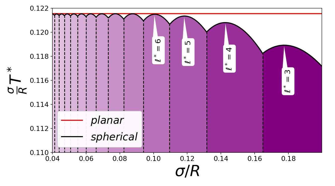
The $\lambda$-line itself can be obtained by using equation (13). In figure 4 we plot the maximum temperature $T^{*}$ reached by the $\lambda$-line as a function of the ratio $\sigma/R$, both for the spherical and the planar case. The latter depends trivially on $\sigma/R$ because of the factor $R$ in the two-Yukawa tail of potential (1), so we isolate this factor in order to better show the differences between the two cases.

Similarly to what happens for the GEM4 fluids ²⁵, $\lambda$-line for the spherical system displays kinks corresponding to values of $\sigma/R$ where the position of $\ell^{*}$ shifts (with $\ell^{*}$ being the position of the negative minimum of the potential, or of the maximum of the structure factor). This also has consequences on the structure of the inhomogeneous phases found in each region, although the details of the phase diagram are not uniquely determined by the position of $\ell^{*}$.

Using the functional developed in the previous sections we can now obtain theoretical predictions for the phase diagram of the SALR fluid. We search for the equilibrium density profile for different values of the mean density $\rho$, of the temperature $T^{*}$, and of the ratio between the size of the particles and the radius of the sphere $\sigma/R$.

The boundaries between two phases A and B are obtained by a Maxwell construction, i.e. by imposing the conditions $\mu_{A}=\mu_{B}$, $\beta\Omega_{A}=\beta\Omega_{B}$. The first condition can be rewritten in terms of the trial densities as $\bar{\rho}_{A}=\bar{\rho}_{B}$. However, since the actual density of the system $\rho$ is obtained a posteriori, we stress that $\rho_{A}$ is not equal to $\rho_{B}$ at the transition, leading to the appearance of a coexistence region that separates the two phases.

We also remark that, as detailed in our previous work ^{25, 40}, one cannot truly have a phase transition on a sphere, as it is a finite system, and even metastable phases can contribute to its thermodynamics. Instead of a discontinuity in the density $\rho$ at the transition chemical potential, one expects a smooth crossover of $\rho$, which roughly corresponds to the coexistence regions defined by the Maxwell construction.

We start by considering the phase diagram in the $\rho-T^{*}$ plane, at $\sigma/R=0.1$ corresponding to $\ell^{*}=6$, which we show in figure 5. Fixing a temperature below the critical one and moving from lower to higher densities, the fluid is initially homogeneous. However as density increases, it undergoes a series of transitions to different cluster crystal phases, in which the particles aggregate into clusters arranged on an ordered lattice. Contrary to the bulk cases ^{3, 9}, where only one kind of cluster crystal is found, the finite size of the sphere leads to the appearance of multiple geometries, characterized by having a different number of clusters ($2$, $6$, $8$, $9$, $10$, or $12$).

As one approaches the center of the diagram, one encounters stripe patterns, in which particles arrange in alternating high density (replete) and low density (depleted) stripes around an axis. At $\sigma/R=0.1$ we observe two such patterns: one with $4$ replete and $3$ depleted stripes, and another, its reciprocal, having $4$ depleted and $3$ replete stripes. We refer to them as the replete and depleted stripe patterns, respectively. Interestingly, contrary to what happens in the bulk in two ⁹ and three dimensions ³, the stripe phases do not reach the top of the diagram, which is instead occupied by the $12$-cluster crystal phase.

At even higher densities, one finds a bubble phase: particles form a percolating matrix in which depleted spots, dubbed bubbles, are arranged in an ordered manner. The $12$-bubble configuration encountered for $\sigma/R=0.1$ corresponds to an inverted $12$-cluster configuration, with bubbles arranged in the same geometry as the clusters.

One can notice a symmetry through the center of the diagram, as phases on either side of the transition between the two stripe phases are the negative of each other: one stripe pattern is depleted where the other is replete, and vice-versa; and the same is true for the $12$-cluster phase and the $12$-bubble phase. This, however, is broken by the presence of the low density cluster phases, which do not have corresponding bubble patterns. An explanation for this behavior will be proposed further on.

Notwithstanding the differences described above, the overall sequence of cluster, stripe, and bubble phases is similar to that found in the two-dimensional bulk ⁹, and in both cases is driven by the presence of the hard-core part of the potential. While in soft-core fluids such as the GEM4 ²⁵ the density inside the clusters can grow indefinitely, and clusters actually become more localized as particles are added to the system, in the SALR fluid the hard core prevents particles from overlapping, forcing clusters to grow larger and larger. As the density increases, each phase is superseded by another one with higher packing efficiency. However, for the case at hand of a system confined on a spherical surface, also finite size effects play a role, and entail a wider geometrical variability of such phases, and the presence of topological defects.

In the case of cluster and bubble phases, topological disclination defects can be understood as lattice points having a defective number of nearest neighbors ⁴¹, whereas stripe patterns also contain two disclination defects located at the poles of the sphere ⁴². While the variety of geometries encountered in the phase diagram manifest these topological defects in different ways, all obey the same conservation law which states that ⁴³

$$\sum_{k}q_{k}=\frac{1}{2\pi}\int dS\,G=2,$$

(16)

where the sum is carried over the topological charges of the defects $q_{k}$, and the integral represents the Euler characteristic $\xi=2$ for the $2$-sphere, proportional to the integral of the local gaussian curvature $G$ over the surface. By computing the topological charge of different kinds of disclinations ⁴³, one can easily predict the geometry that will emerge: for instance $12$-cluster crystals must necessarily contain $12$ five-fold disclinations, because their topological charge is $\tfrac{1}{6}$, while stripe patterns always contain two pole disclinations with charge $1$.

Another aspect in which the SALR model on a sphere differs from its bulk counterpart is the aforementioned presence of different cluster crystals for the same value of $\sigma/R$. This also marks a difference with respect to the GEM4 fluid on the sphere considered in a former study ²⁵: in that case, only one kind of cluster crystal was observed at each fixed value of $\sigma/R$, independently of density or temperature. More specifically, our choice of $\gamma_{1}=\tfrac{5}{6}$ was made to obtain $\ell^{*}=6$ at $\sigma/R=0.1$: for this value of $\ell^{*}$ the phase diagram of the GEM4 fluid only contains configurations with $12$ clusters, whereas in the SALR fluid we also observe configurations with fewer clusters, albeit the expected $12$-cluster configuration still occupies the largest portion of the region of the phase diagram inhabited by cluster crystals.

The explanation of this more complex behavior could lie in the presence of the short-range attraction, which allows particles to aggregate into clusters even at low densities, whereas clustering in purely repulsive systems emerges only as a collective behavior at high densities. In fact we even managed to find a metastable phase having a single cluster: this configuration never becomes the equilibrium distribution, as it is superseded by either the 2-cluster configuration or the homogeneous phase at all densities; however, its existence still proves that, contrary to systems with purely repulsive interactions, the attractive part of the SALR potential can indeed stabilize isolated structures.

To further illustrate the differences between the low density and high density behavior of the system, we introduce the local grand potential $\beta\omega_{D}$, which is the grand potential of a single cell in our grid

	$\displaystyle\beta\omega_{D}(\hat{x})=\beta f_{id}+\beta f_{HD}+\beta f_{P}-\beta\mu N$		(17)
	$\displaystyle\beta f_{id}-\beta\mu N=\frac{\pi^{2}}{K^{2}}\rho(\hat{x})\big[\ln(\rho(\hat{x})/\bar{\rho})-1-\beta\mu_{ex}\big]\sin\theta_{\hat{x}}$
	$\displaystyle\beta f_{HD}=\frac{\pi^{2}}{K^{2}}\rho(\hat{x})\big[(1-\eta(\hat{x}))^{-1}+\ln(1-\eta(\hat{x}))-1\big]\sin\theta_{\hat{x}}$
	$\displaystyle\beta f_{P}=\frac{\pi^{4}}{2K^{4}}\beta\rho(\hat{x})\sin\theta_{\hat{x}}\sum_{\hat{x}^{\prime}}\rho(\hat{x}^{\prime})w(\hat{x},\hat{x}^{\prime})\sin\theta_{\hat{x}^{\prime}}.$

In figure 6 we plot the density profiles and the local grand potential around the centers of clusters in different configurations (1 cluster, 2 clusters, and 12 clusters), and at different densities $\bar{\rho}$. We recall that $\bar{\rho}$ does not generally coincide with the actual average density observed in the system, but is an intuitive way of parametrizing the chemical potential.

Isolated clusters at low densities are all surrounded by an unstable ring, denoted by a positive local grand potential at the interface between the cluster itself and the depleted exterior: this is due to a smaller number of neighbors for particles at the interface, as well as to the repulsive tail of the potential of particles at the center of the cluster. However, the presence of a local frustration actually helps the overall structural integrity of the cluster: the number of frustrated particles is proportional to the diameter $\gamma$ of the cluster, while the surface of the cluster itself is proportional to $\gamma^{2}$. Because of this, splitting a cluster into two smaller ones covering the same area leads to an increase of the number of frustrated particles proportional to $\sqrt{2}$.

Interestingly, the 12-cluster crystal does not display this characteristic at higher densities: the stability of the configuration is ensured by the presence of neighboring clusters pushing against each other, which also leads to deeper local grand potential wells. Being able to exploit a different clustering mechanism, the SALR fluid displays unexpected cluster phases at low densities, but it recovers the same configurational behavior of the GEM4 fluid at higher densities, where collective effects become dominant. This also offers an explanation for the asymmetry of the phase diagram, i.e. the absence of $2$, $6$, $8$, $9$, and $10$-bubble phases: bubble configurations only rely on collective effects for stability, exploiting the long-range repulsions between particles. This only allows the formation of patterns with the symmetry dictated by $\ell^{*}$.

This can be seen in figure 7, where we analyze some of the quantitative features of the inhomogeneous phases, measured at $T^{*}=0.5$ and $\sigma/R=0.1$. We also compare the properties of the stable phases to those of two metastable ones, shown at the bottom of the figure: a single cluster phase and a helix phase, which we were able to obtain thanks to the unconstrained minimization algorithm we employed. Helix phases have been previously observed in SALR fluids, not only on spherical surfaces ^{16, 44}, but also in 3D systems confined inside pores of various shapes ^{45, 46}. Contrary to what reported for the cases considered there ^{16, 45}, however, the helix phase which we observe is never the equilibrium distribution on the sphere.

In the top panel we compare the total power at harmonic degree $\ell^{*}=6$, $P_{\ell^{*}}=\sqrt{\sum_{m}\rho^{2}_{\ell^{*},m}}$ of different phases. This quantifies the degree to which the geometry of the observed patterns overlaps with spherical harmonics of degree $\ell^{*}$, all characterized by the same overall periodicity.

We observe that, at high density, the range over which a phase is stable roughly corresponds to the range of densities at which its $P_{\ell^{*}}$ is the largest among those of the other phases. However this is not quite true at lower densities, further emphasizing the presence of two different stability mechanisms between the two regimes. The helix phase, which is only present at higher densities, has a much lower $P_{\ell^{*}}$ with respect to the other phases and never becomes the equilibrium one. This suggests that phases with a large $P_{\ell^{*}}$ are better able to exploit the characteristic lengthscale introduced by the potential and thus be more stable.

In the middle panel we show the maximum packing fraction for the various phases. For all configurations $\eta$ is much smaller than the close-packing fraction on the plane: this physical behavior is recovered despite the fact that $\eta_{CP}\simeq 0.9069$ is not a parameter of our density functional theory, in fact according to the scaled-particle approximation used here, all values of $\eta$ up to $\eta=1$ would be allowed. Notice that here we refer to the planar value for the close-packing fraction of hard disks, because its spherical counterpart depends on the number of particles and is not known for large ensembles ^{47, 48}. One can also notice that the densities achieved by the system inside the mesoscopic structures are compatible with crystal states ⁴⁹, although we are not able to probe their internal structure due to the local density approximation.

Finally, in the bottom panel we show the typical size $\gamma$ of the mesoscopic structures, measured as the half width at half maximum of the high density patches for the cluster, replete stripe and helix phases, and of the low density patches for the depleted stripe and bubble phases. Interestingly, none of the lower density cluster phases (i.e. all except the $12$-cluster crystal) are stable beyond $\gamma/\sigma=3$, which roughly corresponds to the position of the maximum of the tail potential, as shown in figure 1. For higher density phases we observe that symmetric patterns (i.e. $12$ clusters and $12$ bubbles, or replete stripes and depleted stripes) display a roughly symmetrical behavior of $\gamma$, simply because depleted patches become smaller and smaller as particles are added to the system.

Next we consider the phase diagram in the $\rho-\sigma/R$ plane, at fixed temperature $T^{*}=0.5$, shown in figure 8. The homogeneous fluid occupies the low and high density regions, but the middle section of the diagram is occupied by a plethora of inhomogeneous patterns. We can partition this region into three domains: at lower densities we encounter cluster crystals, the middle portion is occupied by stripe patterns, and at high densities we find bubble phases. As observed for the phase diagram in the $\rho-T^{*}$ plane, one can trace an approximate symmetry axis passing through the middle of the stripe region, so that phases on opposite sides, excluding the cluster crystals at low densities, are the negative of each other. In particular one notices that some of the stripe phases are their own negative, so that they extend over a larger region on the two sides of the symmetry axis.

We also notice that, as for the previously studied GEM4 fluid ²⁵, the equilibrium phases are roughly determined by the value of $\ell^{*}$. For example, the region of stability of each stripe pattern roughly corresponds to a single $\ell^{*}$ domain of figure 8. Cluster crystal phases, instead, display a peculiar behavior, whereby at low densities they extend a tail into regions of lower $\sigma/R$. This means that cluster phases characterized by a smaller $\ell$ and a larger inter-cluster distance than the optimal ones for the value of $\sigma/R$ at hand do not disappear abruptly, but still survive at low density, in line with the discussion of the case $\sigma/R=0.1$ carried out above.

We conclude our assay of the phase diagram by remarking that the phases we find are qualitatively consistent with previous studies of the SALR model through MC simulations ¹⁶, albeit some differences in the implementations of the SALR potential prevent us from comparing the phase diagram to the phases found in that study on a one to one basis. While we are able to find some interesting metastable patterns (such as the single cluster phase, or the helix phase), we did not observe labyrinth patterns or stable helix phases ^{16, 45}. At least in the case of labyrinth patterns, our inability to locate them may be due to the fact that we consider values of $\sigma/R$ much larger than those at which these phases are predicted to occur (i.e. $\sigma/R=0.01$ ¹⁶).