Ultraviolet Spectropolarimetry with Polstar: Massive Star Binary Colliding Winds
Abstract
The winds of massive stars are important for both their direct impact on the interstellar medium, and their influence of the final state prior to supernova. However, the dynamics of these winds is understood primarily via their illumination from a single central source. The Doppler shift seen in resonance lines is a sharp tool for inferring these dynamics, but still the mapping from that Doppler shift to the radial distance from the source is ambiguous. Binary systems can reduce this ambiguity by providing a second light source at a known radius in the wind, seen from orbitally modulated directions. A massive companion also provides unique additional information about wind momentum fluxes, from the nature of the collision between the winds. Since massive stars are strong ultraviolet (UV) sources, and UV resonance line opacity in the wind is strong, UV instruments with high resolution spectroscopic capability are essential for extracting this dynamical information. Also, polarimetric capability helps further resolve ambiguities in aspects of the wind geometry that are not axisymmetric about the line of sight, because of its unique access to scattering direction information. We review how the proposed MIDEX-scale mission Polstar can use UV spectropolarimetric observations to critically constrain the physics of colliding winds, and hence radiatively-driven winds in general. We propose a sample of 20 binary targets, capitalizing on this unique combination of illumination by companion starlight, and collision with a companion wind, to probe wind attributes over a range in wind strengths. Of particular interest is the hypothesis that the radial distribution of the wind acceleration is altered significantly, when the radiative transfer within the winds becomes optically thick to resonance scattering in multiple overlapping UV lines.
I Introduction
Despite comprising the rarest stellar mass group, massive stars ( 8 M⊙) are amongst the most important originators of elements in the Universe because they synthesize and distribute heavy elements, especially oxygen through aluminum, when they explode as supernovae. They also form and evolve much faster than lower-mass stars, thereby influencing the formation and composition of all other stars and their planets. The drastically stronger stellar wind of a massive star, when compared to the solar wind, also enriches the interstellar medium, and can lead to significant changes in the star’s mass over its lifetime. This affects its evolutionary path in the H-R diagram, its type of supernovae, whether it becomes a gamma-ray burster, and the compact remnant it produces, along with any gravitational wave signature it might create if it is a close binary.
Indeed, most massive stars spend a large fraction of their lives in binary systems with other massive stars, and more than half are thought to engage in mass exchange with a close companion (Sana et al. 2012). Tracking these evolutionary effects are the topic of two other Polstar proposal objectives, called S3 (Jones et al. 2021) and S4 (Peters et al. 2021); this white paper relates to objective S5, which entails using the proximity of the two massive stars as a unique probe of the nature of their wind dynamics.
I.1 Wind Acceleration and Stratification
Over the past few decades our understanding of radiatively-driven hot, massive-star winds has greatly improved. But despite this observational and theoretical progress, fundamental details of radiatively driven winds, such as the velocity structure, still elude us. The so-called , although extremely convenient to describe the general density structure of massive-star winds, does not arise from a solid physical description of the winds; it rests on an unlikely simplification that the wind opacity does not undergo significant change as the wind temperature and density drop with radius, and as the radiation field shifts from primarily diffusive to primarily radially streaming. Attempts to better describe the radial acceleration profile of hot-star winds have been made over the years, such as adjusting the value of the exponent, or in the case of WR stars, adopting a typical value of that exponent in the inner wind, while using in the outer wind a higher value describing a second extended acceleration regime (Hillier & Miller 1999; Gräfener & Hamann 2005).

.
The radial dependence of the wind speed has important consequences, as it controls the steady-state density structure, and creates the diagnostically significant mapping from observable Doppler shift to radial location. In optically thick outflows such as those of WR stars, the detailed wind structure is even more important, because the hydrostatic surface of the star is hidden from view, leaving the wind as the only layer of the star that is directly accessible to observation. Dense winds also experience additional opacity changes as the temperature drops significantly and the radiation field shifts from being highly diffusive in deep layers to more free streaming in outer layers. Therefore, we wish to test the hypothesis that the different character of radiative transport and opacity gradients in denser winds, compared to less dense winds, changes the nature of the acceleration as a function of radius. This white paper describes how this test can be carried out in a special sample of colliding-wind binary systems.

I.2 Making Use of Massive Stars in Binaries
Massive stars in binaries offer a unique opportunity to improve our understanding of radiatively driven winds. We can use the light from one star to probe the wind of the other star, allowing us to study the structure of its wind, which provides information on its density, the velocity law, the acceleration zone, and the ionization structure. This method has long been successfully used in the past to investigate, for example, the nature of WR stars citep1993ApJ…415..298S.
An even older version of this approach that focused on light curves (Cherepashchuk et al. 1984) from the WN5 + O6 V eclipsing binary V444 Cygni, covering the wavelength range from to 3.5 , demonstrated that the WN5 star was hot (90,000 K), compact (), and had an outflowing atmosphere in which the temperature decreased smoothly with height. This helped resolve a long-standing controversy in the nature of Wolf-Rayet stars. Additional studies have investigated the stratification in the atmosphere (Eaton et al. 1985; Brown & Shore 1986, e.g.,), and revealed, for example that Fe v in the wind of the WR star contributed to the atmospheric eclipse signal in the UV.
Koenigsberger & Auer 1985 used observations of 6 WR+O systems to show the extended WR atmosphere eclipsed the O stars, and used it to provide constraints on the atmosphere. A further analysis of four binaries by Koenigsberger 1990 showed that the Fe iv/Fe v ratio decreased with radius, and that the wind was still being accelerated at 14 . Auer & Koenigsberger 1994a completed a detailed study and showed how line profile variations could be used to investigate the structure of the winds. Thus, select binary systems have a history of generating breakthrough studies of hot stars, a spirit that is extended into the present in this white paper.
I.3 The Diagnostic Potential of Wind Eclipses
For a given binary configuration, spectroscopic variations are caused by the absorption of the light from one star by the atoms in the wind of the other. Previous UV spectroscopy has shown that absorption occurs mainly in low-excitation and resonance transitions of abundant ions (Koenigsberger & Auer 1985, e.g.). Therefore, these were called selective wind eclipses. As shown in Figure 1, for the WR+O binary Velorum (St-Louis et al. 1993), many ions show a symmetric absorption profile spanning positive and negative velocities in the difference spectrum between phases 0 (WR star in front) and 0.5 (O star in front), as expected. However, note that for certain lines, such as the semi-forbidden C iii] 1909 line and the entire forest of Fe iv lines, only absorption at negative velocities (towards observer) is observed. This unexpected behaviour still remains to be explained.
Examination of the times series for the same star of lines that behave more as expected has shown that the absorption profile is widest when the O companion is directly behind the WR star (called phase 0), and becomes narrower as it orbits to a perpendicular direction with the line-of-sight (phase 0.5). This is seen in Figure 2) by considering the difference between the line profile at the phase shown for the well-isolated C iii 2297 line, and that line seen when the O companion is nearly perpendicular to the WR star. Here there is evidence of wind eclipse when the O star is seen through the WR wind, at both red and blue Doppler shifts, spanning the range of projected velocities in the WR wind.
The detailed shape of the eclipse profile in the various transitions will be determined by the opacity encountered by the light from the companion star on its way to the observer and therefore on the projected velocity and ion abundance. As the companion moves through its orbit, different parts of the wind are probed as the line-of-sight differs for different configurations. This allows to probe different regions of the flow as a function of distance from the center of the star. If the two stars have strong winds, each one can act as a probe for the wind of the other. The combination of all resulting eclipse profiles observed at each position of the orbit contains information on the velocity, density and abundance structures of the wind.
Because of the presence of strong resonance lines of several abundant ions (e.g., due to C iv, Si iv), far ultraviolet spectroscopy is an ideal tool to study massive-star winds and particularly the spectroscopic variations originating from selective wind eclipse. Emission at any given frequency probes a large volume of the wind where as absorption features primarily probes material along the line of sight to the star. The shape of the continuum light-curve over the binary orbit also allows to probe the column depth of the wind. The opacity of O and WR star winds at optical and UV wavelengths is primarily due to electron opacity. In WR stars Fe lines in the UV create a pseudo“continuum”, and these also contribute significantly to the opacity.
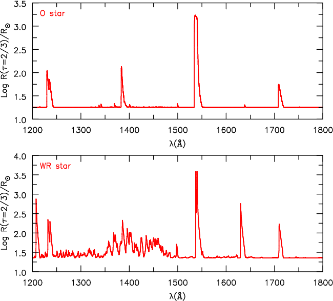
In Figure 3 we illustrate the location at which a radial optical depth of 2/3 occurs as a function of wavelength for an O star and a WR star. The minimum radius, at these wavelengths, is set by electron scattering. At other wavelengths we see the influence of strong bound-bound transitions. The Fe forest is particularly prevalent in the WR star. While the actual numerical values are dependent on the adopted stellar radius, effective temperature and mass-loss rate, the plots do show how different wavelengths have the potential to be used as diagnostic probes in binary star systems.
I.4 Colliding Winds in Massive Binaries
Another aspect of close massive binaries is that the winds of the two stars collide forming a shock-cone structure, generating an asymmetric gas distribution. Colliding-wind binaries (CWB) can teach us a great deal about the individual stars and their winds because the geometry of the interaction region is strongly dependent on the component winds. Indeed, the details of the geometry and physical characteristics of the shock structure depend on the physical parameters of the individual winds, such as the mass-loss rate and velocity structure, thereby providing a further probe of these parameters.
Early theories describing these binaries used momentum flux (Girard & Willson 1987, e.g.) and ram-pressure balance (Kallrath 1991, e.g.), or hydrodynamic models (Stevens et al. 1992, e.g.), until Cantó et al. 1996 produced a complete analytical description in the limit of rapid shock cooling (see Section III.1). Further work in the area has focused on hydrodynamic simulations (Parkin & Pittard 2008; Lamberts et al. 2011; MacLeod & Loeb 2020) and predictions of line profiles in both optical (Luehrs 1997; Ignace et al. 2009; Georgiev & Koenigsberger 2004) and X-rays (Rauw et al. 2016; Mossoux & Rauw 2021). The result of these models, combined with a number of phase-resolved observations (Williams et al. 1990; Tuthill et al. 1999; Rauw et al. 2001; Sana et al. 2001; Rauw et al. 2002; Sana et al. 2008; Gosset et al. 2009; Parkin et al. 2009; Williams et al. 2009; Kennedy et al. 2010; Lomax et al. 2015; Nazé et al. 2018; Williams 2019; Callingham et al. 2020, e.g.), is that we have a good understanding of the expected geometry of colliding winds.
However, collision of the winds will additionally induce complex geometric structures that must be carefully analyzed to be able to extract the desired diagnostics. In this context, purely spectroscopic information may not suffice to resolve the potential ambiguities in such a complex structure, including the location and density of the bow shock, the inclination of the orbit, and the potential for asphericity in the intrinsic winds.
Polarimetric observations are thus a vital tool for revealing details of the mass-loss and mass-transfer structures in these binaries. Both continuum emission (arising from the stars) and line emission (arising from winds, CIRs, or other shock regions) may be polarized in a CWB system via scattering from wind clumps (Harries et al. 1998; Davies et al. 2005), accretion disks (Hoffman et al. 1998), jets (Fox & Hines 1998), bow shocks (Shrestha et al. 2018; Shrestha et al. 2021), and other asymmetric distributions of material or velocities within the system (Schulte-Ladbeck et al. 1992; Villar-Sbaffi et al. 2005; Fullard et al. 2020). Because scattering near the orbital plane tends to produce repeatable effects over many binary cycles, spectropolarimetric monitoring allows us to reconstruct the 3-D shapes of the regions scattering both continuum and line emission (e.g., St-Louis et al. 1993; Lomax et al. 2015; Fullard et al. 2020).
Given that massive star winds are strongly ionized, it is reasonable to consider Thomson scattering as the dominant scattering method for photons in the winds, which in turn can polarize the observed light. The resulting polarization is sensitive to the geometry of scattering regions but also depends on the chemical composition of the wind and its stratification as this will strongly affect the number of available scatterers. Therefore modeling polarimetric observations is a powerful tool to inform us about the geometry and density structures of the colliding winds in interacting systems. This information is critical to our understanding of the roles of binary stars in enriching the ISM and producing explosive transients and gravitational-wave sources.
The classic Brown et al. 1978 model approximates the time-varying continuum polarization caused by the illumination of stellar winds in a binary system viewed at an arbitrary inclination angle. In this model, the scattering region is described as an optically thin electron gas. The envelope pattern is assumed to co-rotate with the illumination sources, appropriate for steady-state systems in circular orbit. The illuminators consist of one point source at the center of the scattering region and an additional external point source representing the companion.
Brown et al. 1982 extended the BME model to consider elliptical orbits, and Fox 1994 further extended the formalism to consider finite illuminators. Fox 1994 showed that occultation is only important in very close binary systems, where separation is less than 10 times the radius of the primary. Hoffman et al. 2003 quantified the polarization produced by external illumination of a disk in a binary system. However, none of these enhancements to the theory included the effects of colliding winds in the time-dependent polarization results. St-Louis et al. 1993 and Kurosawa et al. 2002 modeled the polarization variations in the colliding-wind system V444 Cyg. Also, spectroscopic analysis of wind eclipses in general and for this system in particular have been carried out (Auer & Koenigsberger 1994b), but the results have not been compared across a range of binary parameters to extract the important trends. Harries et al. 2000 used a Monte Carlo formalism to estimate the polarisation caused by the scattering off dust and electrons in a colliding-wind shock cone if it were present in the long-period binary WR137 and found that for such a wide binary, the level would be very small (0.03% ). Notwithstanding these individual efforts, a general formalism has not yet been produced.
The Polstar team includes several experts in polarimetric modeling who will focus on developing the necessary tools to derive physical results from spectropolarimetric signatures. Polarization simulations of bow shocks, which polarize light both when illuminated by a central source and when the light originates within the shock itself (Shrestha et al. 2018; Shrestha et al. 2021), can be incorporated into binary models, as we discuss below. We will also investigate the effects of the wind collision regions and the distributed nature of line emission on the wavelength dependence of polarization. Given that complex continuum and line polarization signals associated with CWBs have been observed in several systems (St-Louis et al. 1993; Lomax et al. 2015; Fullard et al. 2020) and are likely to occur in the UV as well (Schulte-Ladbeck et al. 1992; Hoffman et al. 1998), such modeling efforts are critically important.
We intend to use Polstar to secure extensive UV spectropolarimetric timeseries of key massive binary systems in crucial lines with observations well-distributed around the orbital cycle. Having multiple diagnostics is important – different diagnostics probe different regions of the flow and trace different physics. For example, P Cygni absorption (blue shifted absorption associated with a redshifted emission profile) only samples material along our line of sight. Conversely, the emission line samples a much large volume. Continuum polarization, to some extent, is influenced by the whole volume. Optical studies do not have the necessary lines for the studies proposed here. A well-distributed time series is also crucial, since spectra taken at different times probe distinct orientations of the binary system. The combination of polarimetry and UV spectroscopy, almost unexplored, offers a unique opportunity to resolve ambiguities left by either approach alone. For example, the rate of change of the polarization position angle caused by the colliding wind interaction is a diagnostic of the orbital inclination that is complementary to light-curve considerations.
I.5 Small and Large-Scale Structure in Radiatively-Driven Winds
Growing observational evidence suggests that radiatively driven outflows are highly clumped, including the telltale presence of small sub-peaks observed to move from the center to the edges of strong emission lines in both O stars (Eversberg et al. 1998, e.g.,) and Wolf-Rayet (WR) stars (Lépine & Moffat 1999, e.g.,). Inconsistencies in line strengths (Hillier et al. 2003; Crowther et al. 2002; Massa et al. 2003; Fullerton et al. 2006, e.g.,) and the relative strength of electron scattering wings to their adjacent profiles (Hillier 1991; Hamann & Koesterke 1998, e.g.) also indicate that the winds are clumped. Large-scale structures are also thought to be present in the winds of most, if not all, OB stars, as shown by the presence of NACs and DACs in their ultraviolet spectra (Howarth & Prinja 1989; Kaper et al. 1996, e.g.,) that are thought to be the observational signature of Corotating Interaction Regions (Cranmer & Owocki 1996; Mullan 1986, CIRs,).
These important structural effects are the subject of a different white paper (Gayley et al. 2021), but can be further elucidated by the special diagnostics available in colliding-wind binaries. Small and large-scale wind structures change the density structure of the winds, and this influences the nature of the wind acceleration being probed in this white paper. Further, winds may be porous both spatially (porosity) and in velocity space (Oskinova et al. 2007; Owocki 2008, called vorosity;). Spatial porosity affects both line and continuum radiation transfer whereas vorosity, which refers to gaps in velocity space, only effects line transfer. These phenomena lead to uncertainties in derived parameters such as mass-loss rates, luminosities, radii, and abundances. In turn, this limits our ability to place accurate constraints on stellar and galactic evolution. As will be seen below, two very bright systems ( Velorum and Ori) that will be targeted for close examination for clumping effects are also targeted here by virtue of their binary status, and these systems will be especially informative when the Polstar diagnostics utilized in the two objectives are combined.
I.6 Mass-loss rates
Mass-loss rates included in stellar evolution calculations typically use a fitting law with an adjustable parameter (Paxton et al. 2011; Meynet et al. 2015, e.g. MESA or Geneva code, ). These laws are based on a combination of theoretical and observational studies of mass loss in O stars. For radiatively-driven winds of hot stars, the theoretical mass-loss rates of Vink et al. 2001 and Nugis & Lamers 2000 are typically adopted. For more luminous stars, they are in rough agreement (factor of 2) with empirically derived mass-loss rates, but for late O stars the rates can differ by an order of magnitude. Even factor of 2 uncertainty is a significant problem for understanding how massive stars evolve and effect their environment.
Observational mass-loss rates are generally derived using an empirical velocity law, and by necessity one is forced to make assumptions regarding the inhomogeneity of the wind (Hillier et al. 2003; Bouret et al. 2012; Sander et al. 2012; Shenar et al. 2015, e.g.,). Typically, the wind is assumed to be clumped, with a fraction occupied by the clumps. Porosity is generally ignored, and the interclump medium is assumed to be void. To first order, empirical modeling derives . Constraints on can be placed by using the strength of electron scattering wings in WR stars, and by using P Cygni profiles in O stars. The latter, however, is more uncertain because of the effects of porosity and vorosity.
Current radiative transfer codes can, potentially, derive the velocity law and mass-loss rates from first principles (Vink et al. 2001; Sander et al. 2020; Björklund et al. 2021; Vink & Sander 2021, e.g.,). However such codes make assumptions about clumping, and may use approximate radiation transfer techniques such as the use of the Sobolev approximation (Sobolev 1960). Further, there are still uncertainties about the nature and role of microturbulence at the sonic point (Hillier et al. 2003; Lucy 2007), and the role of inflation, convection and density inhomogeneities in optically thick regions of the flow (Ishii et al. 1999; Petrovic et al. 2006; Cantiello et al. 2009; Gräfener et al. 2012; Grassitelli et al. 2016, e.g.,). Finally there are uncertainties in the atomic data.
As a consequence of these uncertainties, spectra derived from models constructed on first principle generally do not provide a good fit to observed spectra. At best, mass-loss rates must be regarded as uncertain to at least a factor of two, and in some cases the uncertainty is much larger. However, a factor of two variation in mass-loss rate can have a strong influence on a star’s evolution. This is seen in theoretical calculations (Maeder 1981, e.g.,), and is likely illustrated by the different massive star populations in the LMC and Galaxy, as line-driven mass-loss rates depend strongly on metallicity (Vink et al. 2001, e.g.). Accurate mass-loss rates require an understanding of the density structure, which connects to the velocity structure and the physics of wind driving. Thus the objective considered in this white paper is also relevant to establishing more accurate mass-loss rates in specially selected systems, using the unique diagnostics available in these binary systems.
II PolStar Capabilities and Data Products
Using Polstar (Scowen et al. 2021), we intend to probe the details of the wind density of the stars in these systems by using the light from the other star as a probe. Because the presence of two stars with strong winds in a binary generally leads to the formation of a shock-cone structure, we must also take this into account and actually we intend to use it to further constrain the physical characteristics of the outflows. Finally, companion stars are also not independent light sources – their radiation field can modify the wind of the other star, and in close binaries one or both winds may not reach terminal speed either because of the collision or because of the companion’s radiation field. Radiative braking, the deceleration of one wind by the radiation field of the secondary, will modify the location and structure of the bow shock. The combination of UV spectroscopic time series, polarimetric observations, and spectra modeling will ultimately allow us to constrain the mass-loss rates to unprecedented accuracy.
Phase-dependent observations of systems with elliptical orbits or with different separations will allow us to investigate how the radiation field of one star influences the wind of the second star. Our strategy to address these questions is to study a wide range of wind densities in binary systems with high enough inclination and short enough periods for the companion light to be seen deeply through the primary wind. For the brighter stars, we intend to obtain a full phase coverage of ultraviolet spectropolarimetric observations for each system at the highest possible spectral resolution. Depending on the brightness of a given target, we can bin the spectral resolution as necessary to secure sufficiently high quality signal-to-noise to identify telltale spectral features and polarization variability, with good phase coverage.
We have identified a sample of 20 massive binary systems for which there is evidence in the literature of the presence of a colliding wind structure, and which can be observed with Polstar. These are listed in Table 1.
| Star | HD number | Type | Period (d) | V | UV Flux* | Ch. 1 | Ch.2 |
| exp time(s) | exp time(s) | ||||||
| Ch.1 spec., N=1 | |||||||
| and polar. (SNR=3000) | |||||||
| Gamma Velorum | 68273 | WC8+O7.5III-V | 78.05 | 1.83 | 263 | 2000 | 60 |
| Delta Ori | 36486 | O9.5II+BO5.III | 5.7 | 2.41 | 147 | 3550 | 60 |
| 29 CMa | 57060 | O7Iaf+O9 | 4.4 | 4.95 | 7.5 | 70200 | 60 |
| Ch.1 spec., N=1 (SNR=100) | |||||||
| Ch. 2 polar. (SNR=3000) | |||||||
| Plaskett | 47129 | O7.5I+O6I | 14.4 | 6.06 | 1 | 600 | 1840 |
| WR22 | 92740 | WN7h+O9III-V | 80 | 7.16 | 1.1 | 510 | 1680 |
| 152248 | O7.5III(f)+O7III(f) | 5.8 | 6.05 | 0.8 | 720 | 2300 | |
| WR79 | 152270 | WC7+O5-8 | 8.89 | 6.95 | 0.5 | 1150 | 3680 |
| 149404 | O7.5If+ON9.7I | 9.8 | 5.52 | 0.5 | 1150 | 3680 | |
| Ch.1 spec., N=1.5 (SNR=100) | |||||||
| Ch. 2 polar. (SNR=3000) | |||||||
| WR133 | 190918 | WN5o+O9I | 112.8 | 6.7 | 0.35 | 1110 | 585 |
| WR42 | 97142 | WC7+O5-8 | 7.886 | 8.25 | 0.22 | 1800 | 930 |
| Eta Car(2020) | 93308B | LBV | 2022.7 | 6.21 | 0.2 | 1950 | 1050 |
| WR 25 | 93162 | O2.5If*/WN6+O | 208 | 8.84 | 0.13 | 4020 | 1590 |
| WR140 | 193793 | WC7pd + O5.5fc | 2895.0 | 6.85 | 0.1 | 4020 | 2100 |
| 93205 | O3.5 V((f)) + O8 V | 6.0803 | 7.75 | 0.1 | 6300 | 2100 | |
| Ch.1 spec., N=3 (SNR=100) | |||||||
| Ch. 2 polar. (SNR=1000) | |||||||
| WR137 | 192641 | WC7+O9e | 4766 | 8.15 | 0.04 | 5100 | 5100 |
| HD5980 | 5980 | WN4+O7I | 19.3 | 11.31 | 0.04 | 5100 | 5100 |
| V444 Cygni | 193576 | WN5+O6II-V | 4.21 | 8 | 0.02 | 11100 | 11000 |
| WR69 | 136488 | WC9d+OB | 2.293 | 9.43 | 0.015 | 15600 | 13680 |
| WR127 | 186943 | WN3b+O9.5V | 9.555 | 10.33 | 0.012 | 21400 | 17160 |
| WR21 | 90657 | WN5o+O4-6 | 8.25443 | 9,76 | 0.011 | 22800 | 18720 |
*UV Flux at 1550A ( erg/s/cm2/Å)
at 1500Å, D=60 cm, R=30000/N for spectroscopy
II.1 Spectroscopic Experimental Design
In order to monitor the spectroscopic variability caused by selective wind eclipses and the presence of a colliding wind shock cone and to capture all the subtleties of the phase-related changes, we will use Polstar to secure a series of 10 high-resolution spectra, well-distributed over the orbital phase of each binary on our target list. We plan to observe the 8 brightest systems at the highest resolution (R=30000), the 6 next bright binaries at a slightly lower resolution (R=20000) and finally the 6 less UV bright targets at a more moderate resolution (R=10000). Including fainter targets broadens our system parameters and allows us to include especially interesting targets with overlap with other Polstar objectives, such as V444 Cygni, a well-studied WR eclipsing binary, HD5980, for which one component star has recently undergone an LBV-type eruption, WR 69, a system including a WC9 type star that produces dust, and WR 137, a rare system consisting of a WR star and an Oe star (with a decretion disk) in a wide orbit. For the three brightest targets, we require a signal-to-noise ratio (SNR) of 3000 to reach the necessary high polarimetric precision, while also achieving the high spectral resolution needed to detect the details of the selective wind absorption profile, and details of the clumpy nature of the winds and of the colliding-wind shock-cone. For the other systems, we aim for a SNR of 100 (already 5-6 times higher that what is currently available from IUE data), which will still provide excellent quality data. We plan to use the knowledge gained with our test systems to enhance the interpretation of the lower SNR observations.
II.2 Polarimetric Experimental Design
We have selected three massive binaries that are bright in the ultraviolet to observe at the very highest spectroscopic resolution in spectropolarimetry to serve as test cases. These include hot, massive stars having reached different stages of evolution from bright giants to WR type. Although our standard polarization precision for this experiment denoted S5 is , for these unusually bright systems, we aim for a SNR of 3000 in order to be able to detect the very faint polarization signals from the colliding wind shock-cone, down to a precision of . We also plan to observe these targets in channel 2 at lower spectral resolution, and appropriately shorter exposures, in order to characterize the wavelength dependency of the polarization at similar precision. For the other binaries, our strategy is to obtain the highest SNR possible for the UV flux of the target (either 3000 or 1000) but at lower spectral resolution using observations in channel 2. Channel 1 observations at a lower SNR are also important to characterize the wavelength dependency of the polarization. For all polarization measurements of our targets, we will be able to remove the non time-variable but wavelength-dependent interstellar polarization vector from the interstellar medium between each target and the observer, using the method described in Andersson et al. 2021.
III Polarisation modeling
III.1 The Bow Shock Opening Angle and Wind Momentum Ratios
Cantó et al. 1996 present a convenient semi-analytic bow shock model solution for the shock resulting from the collision of two spherical winds at terminal speed. In this model, the bow shock geometry and its surface density is determined by two fundamental ratios:
| (1) | |||||
| (2) |
The distance of the bow shock from the star with the smallest momentum flux along the line joining the two stars, is given by
| (3) |
and the asymptotic opening angle of the cone, by
| (4) |
III.2 Continuum Linear Polarization of Colliding Wind Systems
BME present a complete theoretical construction for thin electron scattering in generalized envelopes with an arbitrary number of illuminating point sources. The two main limitations of BME are in relation to finite star effects, such as occultation, and the explicit assumption of thin scattering. For application to binary stars, the former can be an adequate assumption unless the binary is quite close or eclipsing. Regarding the latter, the Thomson scattering cross-section is relatively small, and so thin scattering is often appropriate. However, for some high-density scattering regions, multiple scattering may modify the resulting polarization (Hoffman et al. 2003; Shrestha et al. 2018). We will employ both analytical models, described in detail below, and Monte Carlo simulations to investigate the full range of possible density distributions.
For massive star binaries, the high temperatures and strong ionizing fluxes ensure the presence of copious free electrons. Thomson scattering is a gray opacity, which suggests initially that flat polarization is to be expected in the continuum. However, a flat polarization is not generally true, particularly for a binary system.
First, there can be changes across line features. The influence of spectral lines come in 3 basic types: (a) photospheric lines, (b) recombination lines, and (c) scattering lines. For the scattering of starlight by electrons in a circumstellar envelope, the polarization is flat across photospheric lines since the relative polarization is constant. The line formation resides at the source, not in the extended circumstellar envelope.
For case (b), the recombination line is taken to form in the circumstellar envelope. It is possible for such line photons to be scattered by the circumstellar electrons. But such photons are not emerging from the star but distributed throughout the envelope, and represent a diffuse source of photons for scattering. Variations in polarization can be complex. As an example, Ignace 2000a explored variations in polarization at H in a Be star disk with a 1-armed spiral density wave: the polarization in the continuum is little affected by the antisymmetric structure, but in H the density-squared emissivity leads to a highly non-symmetric radiation field in the disk. The result is distinct polarimetric behavior within the line as compared to the continuum. Similar effects can occur for colliding wind systems (Fullard 2020).
There is an important limiting scenario for case (b) known as the “line effect” (Schulte-Ladbeck et al. 1990, e.g.,). This is when the recombination line is formed at a large radius and the electron scattering occurs mainly over a more compact region close to the star. In this situation the line photons are little scattered, and strong line emission can contribute to the flux but not or . The result is a reduction in the relative polarization (sometimes referred to as “diluted” polarization).
Case (c) refers to the possibility of scattering resonance lines as an additional polarigenic opacity. Although resonance scattering polarization for stellar winds has been explored in limited applications (Jeffery 1989; Ignace 2000b), the topic has lacked an observational driver. Such effects require a high-resolution UV spectropolarimeter and the computational tools for making predictions of effects and providing fits to data. The data has largely not existed, given that WUPPE was of lower spectral resolution. Polstar will provide new possibilities for case (c), and the team possesses the radiative transfer tools for developing diagnostics that combine both electron and resonance line scattering.
More relevant for UV spectropolarimetry are the chromatic effects in the relative polarization that arise simply from the presence of two stars with different temperatures in a binary. The net polarization from the unresolved binary systems involves a weighted linear sum of the polarized contributions from scattered starlight by each star. Using 1 for the primary (more massive star) and 2 for the secondary (less massive star), the net polarization is of the form:
| (5) |
where
| (6) |
and
| (7) |
and and represent the relative polarization caused by geometric effects from the perspective of each separate star.
Understanding and is aided with an example. Suppose that the primary were surrounded by an axisymmetric disk. This configuration would produce a polarization contribution if there were only one star. However, that same disk is of course not centered on secondary, so starlight from the secondary scattered by the disk produces a different polarization given by the parameter . For thin scattering the total polarization is just the weighted sum .
Therefore, chromatic effects are predicted, despite Thomson scattering being gray. If the stars have different temperatures11 1 If the temperatures of the two binary components are identical, the polarized spectrum will be flat at every wavelength, in the absence of radiative transfer effects., their spectral energy distributions (SEDs) will differ. This leads to a polarized spectrum, , that in general is not flat. In particular, for hot massive stars, the deviation from a flat polarized spectrum occurs mainly in the UV. Thinking simplistically in terms of Planckian stellar spectra, hot OB star spectra in the optical and at longer wavelengths is in the Rayleigh-Jeans regime22 2 The situation is different for WR star that do not follow the Rayleigh-Jeans law owing to significant free-free and bound-free emission from the wind.. In those wavebands, and become constants. But in the UV, where Polstar will operate, the presence of differing Wien peaks ensure that and vary with wavelength, and will not be flat. Formally, is bounded by and , which provides a richer set of constraints for inferring the geometry of the system. Specifically in terms of colliding winds, the UV in general provides new perspectives with spectropolarimetric data relating to the relative location and geometry (e.g., opening angle) of the colliding wind interaction (CWI) region.
For our application to massive colliding wind binary systems, we assume the colliding wind interaction (CWI) is axisymmetric about the line-of-centers joining the two stars. We further assume that the separate winds of the two stars are each spherically symmetric up to the CWI. As a result, in the notation of BME, we have , and the only factors that are nonzero are and .
BME then considered the more limited scenario of a binary system with a circular orbit and corotating envelope. Our approach allows for elliptical orbits (which Brown et al. 1982 later considered), and using Section III.1, we adopt an analytical solution for the CWI from Cantó et al. 1996.
Our team possesses a suite of computational tools for time-dependent hydrodynamical simulation of colliding winds (Russell et al. 2017, e.g.,) and for the radiation transport for synthetic polarization spectra (Hoffman 2007; Huk 2017). Here we explore the BME approach for several reasons. First it generally has applicability to OB+OB star winds where the electron scattering does tend to be thin. It can also have applicability to WR+OB when the CWI is relatively far removed from the WR star so that electron scattering is again optically thin. Finally, solutions for CWIs are complex, depending on a number of variables pertaining both to the stars and to the orbit. BME provides convenient analytic solutions to allow for exploration of a large parameter space. However, for the sake of brevity, we do assume axisymmetry about the line of centers joining the two stars. This is not always the case owing to the Coriolis force (Lemaster et al. 2007). Also our notation departs slightly from BME, although we still employ similar variables.
III.3 Model Prescription
In our model, the winds of the two stars and the intervening colliding wind shock are prescribed using primarily polar coordinates for each star. The primary star33 3 By “primary star”, we refer to the star with the stronger wind momentum, meaning that when the winds are unequal, the bowshock envelopes the secondary star. is assumed to have the stronger wind in terms of momentum flux, , where is the mass-loss rate and is the terminal wind speed. The secondary is then the weaker wind case in terms of this product. We typically use subscripts “1” and “2” for the primary and secondary.
We define the polar coordinates with respect to the axis that is the line of centers between the two stars. Therefore the polar coordinates centered on the primary star are such that in the direction of the secondary. Likewise, the coordinates linked to the secondary star also have in the direction of the primary. Frequently, our approach uses the standard cosine notation, and .

The individual winds are taken to be spherical with densities varying with the inverse square of the distance from the star. There is a vast range of binary systems. In some the CWI forms at radii where both winds are at terminal speed. In others one wind is at terminal speed, and the bow shock forms in the wind acceleration of the other star (perhaps even crashing onto the hydrostatic atmosphere). To explore polarimetric variability from colliding wind shocks, we use the convenient formulation of Cantó et al. 1996 for their semi-analytic bow shock solution for two spherical winds at terminal speed (see Section III.1).
Figure 4 provides a schematic of the binary system with intervening CWI region between the two stars. The radial distance of the bow shock from either star is denoted as and given by
| (8) | |||
| (9) |
where is the separation between the two stars at any moment. Naturally the solution is only valid when . A special quantity is the standoff radius of the bowshock along the line centers, denoted as and .
| (10) | |||
| (11) |
The case corresponds to a planar shock between identical stars and winds, with .
For a particular geometry, as expressed by the wind and orbital properties, and have generally different values but are defined with respect to the same line of centers joining the two stars. While these parameters are not chromatic, as noted above the total polarization can be chromatic because the two illuminating sources will generally have different SEDs, with
| (12) |
This result, in our notation, is equivalent to equations (6a)
and appropriate lines of (7) from BME for our axisymmetric geometry.
III.4 Model Results
III.4.1 Chromatic Effects in the UV
To illustrate chromatic effects, we fixed a particular set of binary parameters while allowing the temperatures of the two stars to vary. The fixed properties lead to and . In this example, the binary components are separated by . The secondary is twice as large as the primary; the two winds have equal speed; the mass-loss rate for the primary is larger than the secondary. Additionally, we took .
To obtain the spectropolarimetric continuum shape, we treated the two stars as Planckian sources with effective temperatures and . We fixed the temperature of the secondary at K. We varied the temperature of the primary from K to K in K intervals, and display the results in Figure 5, where polarization is shown as positive. For purposes of illustration, the usage of “primary” and “secondary” becomes ambiguous as one of the temperatures varies but all other properties remain the same. The point is to highlight the fact that when the stars have different spectral energy distributions, the continuum polarization is not generally constant with wavelength, even though electron scattering is gray. Only when the two stars have equal temperatures is the continuum polarization truly flat.
Note especially that the wavelength varies from the FUV through the optical to 1 micron. For massive stars with typical temperatures well in excess of K, both the primary and secondary can be characterized as following the Rayleigh-Jeans law in the optical, and the continuum is always flat. It is only in the UV that the polarization deviates significantly from a flat profile. For the selected parameters, the polarization actually drops toward the UV when the primary is hotter (i.e., more luminous), owing to the fact that . By contrast, when the secondary is hotter (i.e., more luminous), the polarization increases significantly. Ultimately, for any combination of binary parameters, when the more luminous star in the UV also has the higher polarimetric component, the polarization is enhanced in the UV, and vice versa.

III.4.2 Variable Polarization with Orbital Phase
The polarimetric properties of the colliding wind system depend on the binary separation, . For a circular orbit, the values and are constant. This is not true when the orbit is eccentric. For eccentricity and semi-major axis , the binary separation varies as
| (13) |
where is the orbital azimuth, defined so that corresponds to periastron. Thus and are functions of orbital phase through the variation of , since even for fixed and ratios, the surface density of the CWI changes as well as the extent of the wind for each respective star up to either side of the CWI.
To obtain the variable polarization with orbital phase, we define as the viewing inclination of the orbital plane, so that is a top-down view and is edge-on. The polarimetric variability is determined by
| (14) | |||||
| (15) |
where the polarization position angle relates to orbital azimuth and orbital plane inclination as
| (16) |
The inclination of the line of centers to the viewer’s line of sight is given by
| (17) |
Figure 6 displays a suite of polarimetric variations for binary systems with different values of and . We fitted a linear regression to in the case of a binary with two identical stars (i.e., planar CWI shock) to obtain , normalized so that at . We show model variable polarization curves for inclinations and eccentricities, as labeled. Top is for loops; bottom shows polarized light curves with orbital phase. The line types represent the different eccentricities. At (not shown), all curves would become horizontal lines with only variation but no variation. Note also that .


III.4.3 WR+O Binaries
We calculated and for three scenarios, with a summary of results displayed in Figure 7. The first case is with orbital separation ranging from to for “slow” winds of 1000 km s-1 for both stars. The second case is for fast winds at 3000 km s-1, with all other parameters fixed. The third scenario corresponds to an intermediate wind speed of 2000 km s-1 at a fixed separation of , but with ranging between 1/15 and 1/5.
The upper panel of Figure 7 summarizes the comparison between slow and fast winds. Note that polarizations are negative for our convention of a binary with orbital plane seen face-on, with the line of centers oriented north-south in the sky. In this panel the red lines represent and blue represent . Solid lines are for the fast wind case, and dashed for the slow wind case. The results are plotted against , normalized as indicated. The net result is that the polarization is overall larger for a slower wind, since the density is larger. We find that is roughly constant as changes, indicating that its value is dominated by the relatively extended spherical wind of the WR star, since the CWI is far removed. Since the CWI is relatively farther from the WR star with increasing , becomes smaller with . Consequently, decreases with increasing . The behavior for the O star is that the polarization is dominated by the CWI. The surface density of the CWI shock for the Cantó et al. 1996 solution scales as overall. These is evidenced by the fact that both blue curves appear quite linear in the plot.
For the lower panel of Figure 7, we display the results differently as is allowed to vary between 1/15 and 1/5 and with smaller , the CWI is closer to the O star component. Consider first the dashed and dotted curves in black, for and , respectively. As becomes smaller, is larger, approaching the limit of the strictly spherical wind value. The value of is much lower, and is plotted as scaled up by .
The blue curve in this lower panel represents the ratio of . Its behavior indicates that from geometrical considerations, the contribution to the polarization from the O star wind is much greater than for the WR wind, even more so as becomes smaller. Even though the WR wind has a much higher optical depth scale, the distortion of the scattering envelope from spherical is quite minor from the perspective of the WR star. This is made clear by the red curve, where “shape” is the ratio , and scaled up by . From the perspective of the O component, the scattering envelope is highly distorted.
In combination, these results suggest that at wavelengths where the O star is more luminous, the polarization will overall be larger (biased toward ) than at wavelengths where the WR star is more luminous (polarization biased toward ). Our treatment does have deficiencies, the most important being that we ignore the wind acceleration region, and that we treat the WR wind as optically thin to electron scattering. For the latter, it is clear that the WR wind is already a minor contributor to the polarization when , and a more full treatment of multiple scattering is hardly expected to impact that conclusion. For the former, inclusion of the wind acceleration region and associated density distribution, along with radiative inhibition could certainly change the detailed outcomes. Nonetheless, the present treatment indicates that , another qualitative result that is unlikely to change despite our more simplistic assumptions.

III.5 Linear Polarization Across Spectral Lines
At optical and UV wavelengths it is often a good approximation to assume that electron scattering is coherent in the frame of the electron. However, since the electron is moving (due to both thermal and large scale motions) relative to both the source and observer there will be a wavelength shift in the observers frame (Auer & van Blerkom 1972). Thermal motions can lead to either a decrease or increase in the scattered photon’s wavelength, while scattering by an expanding monotonic flow will always lead to a redshift. These velocity shifts are observed – in P Cygni for example, in which the thermal electron velocities are larger than the wind velocity, the Balmer series, for example, show nearly symmetric broad extended wings centered on the emission profile (Bernat & Lambert 1978). By contrast, in the spectra of many WR stars only a red electron scattering wing is seen, since in these stars the wind velocities are larger than the electron thermal velocities (Hillier 1984).
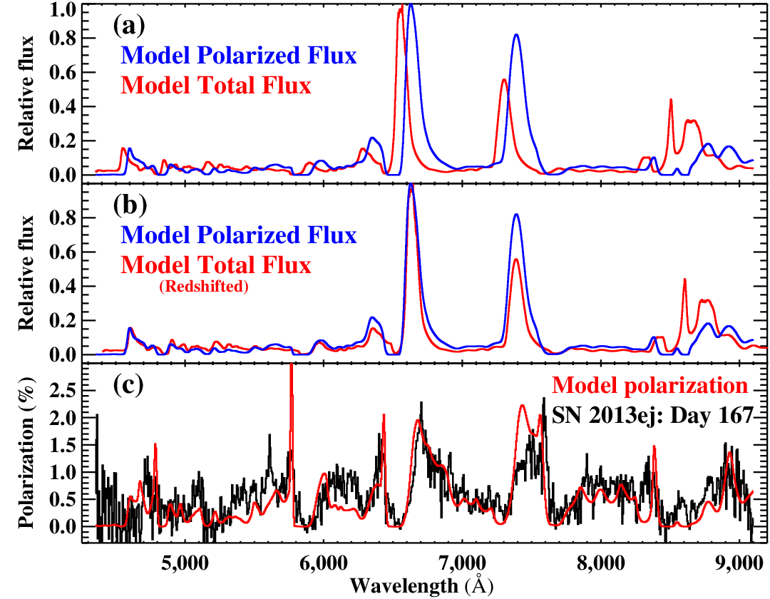
For continuum polarization the velocity shifts induced by electron scattering are generally unimportant. However, they are of crucial importance in understanding line polarization. In Fig. 8 we show an extreme example, taken from polarization studies of supernovae, where the line shift is crucial. In the Type II SN 2013ej the polarized spectrum is very similar to the observed spectrum (Leonard et al. 2021). However, it is different in two important ways: First, the spectrum is redshifted. Second, the agreement between the intrinsic and polarized spectrum depends on which spectral feature is being examined. Both effects are easily understood by assuming that the scattering source is offset from the SN emitting region, and by noting that line emission in a SN region is stratified (different lines originate in different regions of the SN ejecta). Dessart et al. 2021 argued that scattering region was due to a nickel bubble, with an enhanced electron density offset from the center of the ejecta. Due to motion relative to the source, the spectrum is shifted to the red. Furthermore, the similarity between the intrinsic and scattered light will generally be highest for lines arising in the interior regions of the SN ejecta, since in that case the scattering angle is the same, unlike the case where the emission is formed over a much larger volume.
When optically thin electron-scattering is assumed, and other absorption processes neglected (e.g., purely bound-bound transitions), models predict that for an oblate spheroid the polarization should be parallel to the major axis. The reason is simple – more photons will be scattered from the equatorial regions (with their electron vector parallel to the major axis) than the polar regions. However, when optical depth effects are allowed for, the polarization can flip sign, as scattered photons become more isotropic in the higher optical depth equatorial region.
The above scenario is illustrated in 9 where we illustrate the spectrum for a WN Wolf-Rayet star assuming it has an oblate wind with a polar to equatorial density ratio of 0.3. Near 1800 Å, the polarization is positive, as expected for an oblate spheroid. However, around 1400 Å, the polarization is negative, a consequence of Fe-blanketing, which increases total opacity and also introduces line effects. The assumed axial symmetry guarantees that the position angle must be parallel or perpendicular to the rotation axis, so here we have taken the Stokes component to subtract light polarized perpendicular to the rotation axis from light polarized along the axis (and the component at 45 degrees to that would be zero in this symmetry).

Both of the above examples illustrate how the polarization contains important information about the structure of circumstellar matter, whether it be a SN ejecta or a wind. Importantly, we now have the numerical tools to interpret these observations. Polarization, in conjunction with other observations provides an invaluable tool to help understand astrophysical objects, especially since most are spatially unresolved with modern telescopes.
III.5.1 Numerical models
Radiative transfer models are capable of modeling more complex binary phenomena than those allowed by the assumptions of BME (Kurosawa et al. 2002; Hoffman et al. 2003, e.g., ). Leveraging these models is essential for any deep investigation of specific colliding wind systems. Polarization of spectral lines is especially suited to numerical modeling because of how difficult the problem is in asymmetric geometries.
Numerical models can also be used as initial probes much like BME. Because electron scattering is the primary polarigenic mechanism in hot star winds, the effects of line and continuum polarization can be decoupled by considering their emission and scattering regions. A toy model of the well-studied V444 Cyg has been constructed for this purpose (Fullard 2020). It is based on the Kurosawa et al. 2002 E model of the system including a WR star with an appropriate wind density profile from the Potsdam Wolf-Rayet (PoWR) models44 4 See the Potsdam PoWR models at the following website: www.astro.physik.uni-potsdam.de/ wrh/PoWR/powrgrid1.php. A simple spherical cap cutout represents the O star wind (assumed to be of negligible relative density) at the wind collision point, rotated to mimic the effect of orbital motion. Emission occurs from the WR and O star photospheres (where the WR star photosphere is defined from its PoWR model). It reproduces the continuum behaviour of the system as shown in Figure 10.


To represent line polarization caused by Heii, the emission locations are simply changed to originate from a shell in the WR star wind, and from the edge of the shock region in two clumps. The clumps are located at phase and , and lie at the edge of the simulation just beyond the O star orbit. Figures 11 and 12 show the resulting polarization curves compared to existing continuum polarization data. Figure 11 shows the complete wind and shock model, which has a low near-constant Stokes and a similar amplitude of variation in Stokes . Figure 12 shows a model that produces emission only from the two shock regions. This has strong phase-dependent polarization in both Stokes and . Neither model produces polarization similar to the continuum signal. Both show the importance of considering line polarization and its capability to diagnose emission regions in colliding winds. It is clear that obtaining polarization observations specifically in spectral lines will provide additional information than that of the continuum polarization.
IV Conclusions
Colliding-wind binaries are important laboratories for the study of radiative wind driving, and massive stars in general, as the detailed structure and geometry of the interaction region between the winds can yield important information about each component’s individual wind properties. This interaction is not only due to the bow shock, since the wind from each star can also be influenced by the radiation field from the other star. This phenomenon is best studied with a combination of spectroscopy and polarimetry, and as demonstrated above, the ultraviolet provides an ideal bandpass since the spectral energy densities of massive stars peak in that region, leading to a wavelength dependence of the polarization.
Several analytical models provide a satisfactory description of the wind collision region, within certain simplifying assumptions detailed in Sect. III. Our group possesses the ability to leverage these models, as demonstrated for a few illustrative cases.
Using time series of spectropolarimetric observations from Polstar, we will be able to constrain the geometry of the bow shock and therefore the wind properties of a sample of 20 colliding-wind binaries spanning a large parameter space. The obtained dataset will significantly improve upon available observations; spectroscopy will be obtained with much higher signal-to-noise ratio and resolution than with IUE and WUPPE, and with greater polarimetric precision than the latter. Achieving a SNR of 100 at spectral resolution down to the wind sound speed, over an orbitally resolved time domain, opens up new and unique wind dynamics diagnostics, as the light from one star scatters in, and is absorbed by, the wind of the other, with orbitally modulated changes in the relevant angles. These produce a more precise mapping between radius and velocity than possible for single stars, allowing tests of the degree to which different wind types and optical depths alter the wind acceleration and structure formation. Information about the bow shock also constrains the relative momentum fluxes in the winds of the two different stars in the binary.
The work described in this white paper corresponds a single science objective included in the Polstar proposal, which overlaps in interesting ways with several other objectives described in their own white papers. We will take advantage of the ways the unique diagnostics supplied by colliding wind binaries informs these other objectives. For example, Gayley et al. 2021 discuss how Polstar enables the study of structure and clumping in the winds of the brightest targets, in the context of single stars observed continuously over wind dynamical timescales. Two of those targets, Vel and Ori, are binary systems in the colliding-wind target list, so our observations sampled over the system orbit will provide important additional context for the continuous wind dynamics observations. Also, Shultz et al. 2021 explore the global structural effects of strong magnetization in a subset of OB stars, and a particularly important example is Plaskett’s star, which is the only strongly magnetic star observed to also be a rapid rotator. This star is also in our colliding wind target list, and the understanding of its magnetic structure will be complemented by the methods made available by its short-period binary status, as described here.
Closer binaries than the ones examined in this paper can interact and undergo episodes of conservative and nonconservative mass transfer, altering the mass and angular momentum of the binary constituents in ways that are the subject of other Polstar objectives and described in their own white papers. Peters et al. 2021 investigate how UV spectropolarimetry can characterize these mass flows and help determine the fraction of the mass loss by the system, whereas Jones et al. 2021 focus on angular momentum evolution and the pathways for stellar spinup and Keplerian disk creation. UV spectropolarimetry can also provide information regarding the geometry, velocity, and inclination of such disks, as well as the accretion disks of Herbig Ae/Be stars (Wisniewski et al. 2021).
All of these objectives, whose realization will be made possible by Polstar, constrain key evolutionary stages of massive stars and lead to a better understanding of their fates, including the compact objects that they leave behind. Importantly, the analysis of polarization signals from all of these sources will require a detailed understanding of the polarization induced by the intervening interstellar medium; by contributing to improve this knowledge, Polstar will not only enable these topics of stellar physics, but will also yield important insights in the physics of interstellar dust grains (Andersson et al. 2021). Any of these types of systems can, in special cases, provide examples that can be studied over an orbitally modulated range of angles that are either completely sampled, or at least change considerably, over the timeframe of the Polstar mission. This white paper, therefore, is focused on the complementary spectropolarimetric diagnostics available in 20 such cases.


References
- Andersson et al. (2021) Andersson, B.-G., Clayton, G. C., Doney, K. D., et al. 2021, arXiv e-prints, arXiv:2111.08079. https://arxiv.org/abs/2111.08079
- Auer & Koenigsberger (1994a) Auer, L. H., & Koenigsberger, G. 1994a, ApJ, 436, 859, doi: 10.1086/174963
- Auer & Koenigsberger (1994b) —. 1994b, ApJ, 436, 859, doi: 10.1086/174963
- Auer & van Blerkom (1972) Auer, L. H., & van Blerkom, D. 1972, ApJ, 178, 175, doi: 10.1086/151777
- Bernat & Lambert (1978) Bernat, A. P., & Lambert, D. L. 1978, PASP, 90, 520, doi: 10.1086/130376
- Björklund et al. (2021) Björklund, R., Sundqvist, J. O., Puls, J., & Najarro, F. 2021, A&A, 648, A36, doi: 10.1051/0004-6361/202038384
- Bouret et al. (2012) Bouret, J.-C., Hillier, D. J., Lanz, T., & Fullerton, A. W. 2012, A&A, 544, A67, doi: 10.1051/0004-6361/201118594
- Brown & Shore (1986) Brown, D. N., & Shore, S. N. 1986, in ESA Special Publication, Vol. 263, New Insights in Astrophysics. Eight Years of UV Astronomy with IUE, ed. E. J. Rolfe & R. Wilson, 353
- Brown et al. (1982) Brown, J. C., Aspin, C., Simmons, J. F. L., & McLean, I. S. 1982, Monthly Notices of the Royal Astronomical Society, 198, 787, doi: 10.1093/mnras/198.3.787
- Brown et al. (1978) Brown, J. C., McLean, I. S., & Emslie, A. G. 1978, Astronomy and Astrophysics, 68, 415. http://adsabs.harvard.edu/abs/1978A%26A....68..415B
- Callingham et al. (2020) Callingham, J. R., Crowther, P. A., Williams, P. M., et al. 2020, Monthly Notices of the Royal Astronomical Society, 495, 3323, doi: 10.1093/mnras/staa1244
- Cantiello et al. (2009) Cantiello, M., Langer, N., Brott, I., et al. 2009, A&A, 499, 279, doi: 10.1051/0004-6361/200911643
- Cantó et al. (1996) Cantó, J., Raga, A. C., & Wilkin, F. P. 1996, The Astrophysical Journal, 469, 729, doi: 10.1086/177820
- Cherepashchuk et al. (1984) Cherepashchuk, A. M., Eaton, J. A., & Khaliullin, K. F. 1984, ApJ, 281, 774, doi: 10.1086/162156
- Cranmer & Owocki (1996) Cranmer, S. R., & Owocki, S. P. 1996, ApJ, 462, 469, doi: 10.1086/177166
- Crowther et al. (2002) Crowther, P. A., Dessart, L., Hillier, D. J., Abbott, J. B., & Fullerton, A. W. 2002, A&A, 392, 653, doi: 10.1051/0004-6361:20020941
- Davies et al. (2005) Davies, B., Oudmaijer, R. D., & Vink, J. S. 2005, A&A, 439, 1107, doi: 10.1051/0004-6361:20052781
- Dessart et al. (2021) Dessart, L., Hillier, D. J., & Leonard, D. C. 2021, A&A, 651, A10, doi: 10.1051/0004-6361/202140409
- Eaton et al. (1985) Eaton, J. A., Cherepashchuk, A. M., & Khaliullin, K. F. 1985, ApJ, 297, 266, doi: 10.1086/163524
- Eversberg et al. (1998) Eversberg, T., Lepine, S., & Moffat, A. F. J. 1998, ApJ, 494, 799, doi: 10.1086/305218
- Fox (1994) Fox, G. K. 1994, The Astrophysical Journal, 432, 262, doi: 10.1086/174567
- Fox & Hines (1998) Fox, G. K., & Hines, D. C. 1998, MNRAS, 295, 423, doi: 10.1046/j.1365-8711.1998.01296.x
- Fullard (2020) Fullard, A. G. 2020, PhD thesis, University of Denver, United States
- Fullard et al. (2020) Fullard, A. G., St-Louis, N., Moffat, A. F. J., et al. 2020, AJ, 159, 214, doi: 10.3847/1538-3881/ab8293
- Fullerton et al. (2006) Fullerton, A. W., Massa, D. L., & Prinja, R. K. 2006, ApJ, 637, 1025, doi: 10.1086/498560
- Gayley et al. (2021) Gayley, K., Vink, J. S., ud-Doula, A., et al. 2021, arXiv e-prints, arXiv:2111.11633. https://arxiv.org/abs/2111.11633
- Georgiev & Koenigsberger (2004) Georgiev, L. N., & Koenigsberger, G. 2004, Astronomy and Astrophysics, v.423, p.267-279 (2004), 423, 267, doi: 10.1051/0004-6361:200400030
- Girard & Willson (1987) Girard, T., & Willson, L. A. 1987, Astronomy and Astrophysics, Vol. 183, p. 247-256 (1987), 183, 247. https://ui.adsabs.harvard.edu/abs/1987A%26A...183..247G/abstract
- Gosset et al. (2009) Gosset, E., Nazé, Y., Sana, H., Rauw, G., & Vreux, J. M. 2009, A&A, 508, 805, doi: 10.1051/0004-6361/20077981
- Gräfener & Hamann (2005) Gräfener, G., & Hamann, W.-R. 2005, A&A, 432, 633, doi: 10.1051/0004-6361:20041732
- Gräfener et al. (2012) Gräfener, G., Owocki, S. P., & Vink, J. S. 2012, A&A, 538, A40, doi: 10.1051/0004-6361/201117497
- Grassitelli et al. (2016) Grassitelli, L., Chené, A.-N., Sanyal, D., et al. 2016, A&A, 590, A12, doi: 10.1051/0004-6361/201527873
- Hamann & Koesterke (1998) Hamann, W.-R., & Koesterke, L. 1998, A&A, 335, 1003
- Harries et al. (2000) Harries, T. J., Babler, B. L., & Fox, G. K. 2000, A&A, 361, 273
- Harries et al. (1998) Harries, T. J., Hillier, D. J., & Howarth, I. D. 1998, MNRAS, 296, 1072, doi: 10.1046/j.1365-8711.1998.01508.x
- Hillier (1984) Hillier, D. J. 1984, ApJ, 280, 744, doi: 10.1086/162047
- Hillier (1991) —. 1991, A&A, 247, 455
- Hillier et al. (2003) Hillier, D. J., Lanz, T., Heap, S. R., et al. 2003, ApJ, 588, 1039, doi: 10.1086/374329
- Hillier & Miller (1999) Hillier, D. J., & Miller, D. L. 1999, ApJ, 519, 354, doi: 10.1086/307339
- Hoffman (2007) Hoffman, J. L. 2007, in Revista Mexicana de Astronomia y Astrofisica Conference Series, Vol. 30, Revista Mexicana de Astronomia y Astrofisica Conference Series, 57–63. https://arxiv.org/abs/astro-ph/0612244
- Hoffman et al. (1998) Hoffman, J. L., Nordsieck, K. H., & Fox, G. K. 1998, AJ, 115, 1576, doi: 10.1086/300274
- Hoffman et al. (2003) Hoffman, J. L., Whitney, B. A., & Nordsieck, K. H. 2003, ApJ, 598, 572, doi: 10.1086/378770
- Howarth & Prinja (1989) Howarth, I. D., & Prinja, R. K. 1989, ApJS, 69, 527, doi: 10.1086/191321
- Huk (2017) Huk, L. N. 2017, PhD thesis, University of Denver, United States
- Ignace (2000a) Ignace, R. 2000a, in Astronomical Society of the Pacific Conference Series, Vol. 214, IAU Colloq. 175: The Be Phenomenon in Early-Type Stars, ed. M. A. Smith, H. F. Henrichs, & J. Fabregat, 452
- Ignace (2000b) Ignace, R. 2000b, A&A, 363, 1106
- Ignace et al. (2009) Ignace, R., Al-Malki, M. B., Simmons, J. F. L., et al. 2009, A&A, 496, 503, doi: 10.1051/0004-6361:200811214
- Ishii et al. (1999) Ishii, M., Ueno, M., & Kato, M. 1999, PASJ, 51, 417, doi: 10.1093/pasj/51.4.417
- Jeffery (1989) Jeffery, D. J. 1989, ApJS, 71, 951, doi: 10.1086/191404
- Jones et al. (2021) Jones, C. E., Labadie-Bartz, J., Nazé, Y., et al. 2021, arXiv e-prints, arXiv:2111.07926. https://arxiv.org/abs/2111.07926
- Kallrath (1991) Kallrath, J. 1991, Monthly Notices of the Royal Astronomical Society, 248, 653, doi: 10.1093/mnras/248.4.653
- Kaper et al. (1996) Kaper, L., Henrichs, H. F., Nichols, J. S., et al. 1996, A&AS, 116, 257
- Kennedy et al. (2010) Kennedy, M., Dougherty, S. M., Fink, A., & Williams, P. M. 2010, ApJ, 709, 632, doi: 10.1088/0004-637X/709/2/632
- Koenigsberger (1990) Koenigsberger, G. 1990, A&A, 235, 282
- Koenigsberger & Auer (1985) Koenigsberger, G., & Auer, L. H. 1985, ApJ, 297, 255, doi: 10.1086/163523
- Kurosawa et al. (2002) Kurosawa, R., Hillier, D. J., & Pittard, J. M. 2002, Astronomy and Astrophysics, 388, 957, doi: 10.1051/0004-6361:20020443
- Lamberts et al. (2011) Lamberts, A., Fromang, S., & Dubus, G. 2011, Monthly Notices of the Royal Astronomical Society, 418, 2618, doi: 10.1111/j.1365-2966.2011.19653.x
- Lemaster et al. (2007) Lemaster, M. N., Stone, J. M., & Gardiner, T. A. 2007, ApJ, 662, 582, doi: 10.1086/515431
- Leonard et al. (2021) Leonard, D. C., Dessart, L., Hillier, D. J., et al. 2021, arXiv e-prints, arXiv:2110.10875. https://arxiv.org/abs/2110.10875
- Lépine & Moffat (1999) Lépine, S., & Moffat, A. F. J. 1999, ApJ, 514, 909, doi: 10.1086/306958
- Lomax et al. (2015) Lomax, J. R., Nazé, Y., Hoffman, J. L., et al. 2015, A&A, 573, A43, doi: 10.1051/0004-6361/201424468
- Lucy (2007) Lucy, L. B. 2007, A&A, 468, 649, doi: 10.1051/0004-6361:20077298
- Luehrs (1997) Luehrs, S. 1997, PASP, 109, 504, doi: 10.1086/133907
- MacLeod & Loeb (2020) MacLeod, M., & Loeb, A. 2020, The Astrophysical Journal, 902, 85, doi: 10.3847/1538-4357/abb313
- Maeder (1981) Maeder, A. 1981, A&A, 101, 385
- Massa et al. (2003) Massa, D., Fullerton, A. W., Sonneborn, G., & Hutchings, J. B. 2003, ApJ, 586, 996, doi: 10.1086/367786
- Meynet et al. (2015) Meynet, G., Chomienne, V., Ekström, S., et al. 2015, A&A, 575, A60, doi: 10.1051/0004-6361/201424671
- Mossoux & Rauw (2021) Mossoux, E., & Rauw, G. 2021, A&A, 646, A89, doi: 10.1051/0004-6361/202039437
- Mullan (1986) Mullan, D. J. 1986, A&A, 165, 157
- Nazé et al. (2018) Nazé, Y., Koenigsberger, G., Pittard, J. M., et al. 2018, ApJ, 853, 164, doi: 10.3847/1538-4357/aaa29c
- Nugis & Lamers (2000) Nugis, T., & Lamers, H. J. G. L. M. 2000, A&A, 360, 227
- Oskinova et al. (2007) Oskinova, L. M., Hamann, W. R., & Feldmeier, A. 2007, A&A, 476, 1331, doi: 10.1051/0004-6361:20066377
- Owocki (2008) Owocki, S. P. 2008, in Clumping in Hot-Star Winds, ed. W.-R. Hamann, A. Feldmeier, & L. M. Oskinova, 121
- Parkin & Pittard (2008) Parkin, E. R., & Pittard, J. M. 2008, MNRAS, 388, 1047, doi: 10.1111/j.1365-2966.2008.13511.x
- Parkin et al. (2009) Parkin, E. R., Pittard, J. M., Corcoran, M. F., Hamaguchi, K., & Stevens, I. R. 2009, MNRAS, 394, 1758, doi: 10.1111/j.1365-2966.2009.14475.x
- Paxton et al. (2011) Paxton, B., Bildsten, L., Dotter, A., et al. 2011, ApJS, 192, 3, doi: 10.1088/0067-0049/192/1/3
- Peters et al. (2021) Peters, G. J., Gayley, K., Ignace, R., et al. 2021, arXiv e-prints, arXiv:2111.14047. https://arxiv.org/abs/2111.14047
- Petrovic et al. (2006) Petrovic, J., Pols, O., & Langer, N. 2006, A&A, 450, 219, doi: 10.1051/0004-6361:20035837
- Rauw et al. (2016) Rauw, G., Mossoux, E., & Nazé, Y. 2016, New A, 43, 70, doi: 10.1016/j.newast.2015.08.002
- Rauw et al. (2001) Rauw, G., Nazé, Y., Carrier, F., et al. 2001, A&A, 368, 212, doi: 10.1051/0004-6361:20000527
- Rauw et al. (2002) Rauw, G., Vreux, J. M., Stevens, I. R., et al. 2002, A&A, 388, 552, doi: 10.1051/0004-6361:20020523
- Russell et al. (2017) Russell, C. M. P., Wang, Q. D., & Cuadra, J. 2017, MNRAS, 464, 4958, doi: 10.1093/mnras/stw2584
- Sana et al. (2008) Sana, H., Nazé, Y., O’Donnell, B., Rauw, G., & Gosset, E. 2008, New A, 13, 202, doi: 10.1016/j.newast.2007.07.008
- Sana et al. (2001) Sana, H., Rauw, G., & Gosset, E. 2001, A&A, 370, 121, doi: 10.1051/0004-6361:20010221
- Sana et al. (2012) Sana, H., de Mink, S. E., de Koter, A., et al. 2012, Science, 337, 444, doi: 10.1126/science.1223344
- Sander et al. (2012) Sander, A., Hamann, W.-R., & Todt, H. 2012, A&A, 540, A144, doi: 10.1051/0004-6361/201117830
- Sander et al. (2020) Sander, A. A. C., Vink, J. S., & Hamann, W. R. 2020, MNRAS, 491, 4406, doi: 10.1093/mnras/stz3064
- Schulte-Ladbeck et al. (1990) Schulte-Ladbeck, R. E., Nordsieck, K. H., Nook, M. A., et al. 1990, ApJ, 365, L19, doi: 10.1086/185878
- Schulte-Ladbeck et al. (1992) Schulte-Ladbeck, R. E., Nordsieck, K. H., Code, A. D., et al. 1992, ApJ, 391, L37, doi: 10.1086/186393
- Scowen et al. (2021) Scowen, P. A., Gayley, K., Neiner, C., et al. 2021, in Society of Photo-Optical Instrumentation Engineers (SPIE) Conference Series, Vol. 11819, Society of Photo-Optical Instrumentation Engineers (SPIE) Conference Series, 1181908, doi: 10.1117/12.2594267
- Shenar et al. (2015) Shenar, T., Oskinova, L., Hamann, W. R., et al. 2015, ApJ, 809, 135, doi: 10.1088/0004-637X/809/2/135
- Shrestha et al. (2018) Shrestha, M., Neilson, H. R., Hoffman, J. L., & Ignace, R. 2018, MNRAS, 477, 1365, doi: 10.1093/mnras/sty724
- Shrestha et al. (2021) Shrestha, M., Neilson, H. R., Hoffman, J. L., Ignace, R., & Fullard, A. G. 2021, MNRAS, 500, 4319, doi: 10.1093/mnras/staa3508
- Shultz et al. (2021) Shultz, M. E., Casini, R., Cheung, M. C. M., et al. 2021, arXiv e-prints, arXiv:2111.06434. https://arxiv.org/abs/2111.06434
- Sobolev (1960) Sobolev, V. V. 1960, Moving envelopes of stars (Harvard Univ. Press, Cambridge)
- St-Louis et al. (1993) St-Louis, N., Moffat, A. F. J., Lapointe, L., et al. 1993, The Astrophysical Journal, 410, 342, doi: 10.1086/172751
- St-Louis et al. (1993) St-Louis, N., Willis, A. J., & Stevens, I. R. 1993, ApJ, 415, 298, doi: 10.1086/173165
- Stevens et al. (1992) Stevens, I. R., Blondin, J. M., & Pollock, A. M. T. 1992, The Astrophysical Journal, 386, 265, doi: 10.1086/171013
- Tuthill et al. (1999) Tuthill, P. G., Monnier, J. D., & Danchi, W. C. 1999, Nature, 398, 487, doi: 10.1038/19033
- Villar-Sbaffi et al. (2005) Villar-Sbaffi, A., St-Louis, N., Moffat, A. F. J., & Piirola, V. 2005, ApJ, 623, 1092, doi: 10.1086/428830
- Vink et al. (2001) Vink, J. S., de Koter, A., & Lamers, H. J. G. L. M. 2001, A&A, 369, 574, doi: 10.1051/0004-6361:20010127
- Vink & Sander (2021) Vink, J. S., & Sander, A. A. C. 2021, MNRAS, 504, 2051, doi: 10.1093/mnras/stab902
- Williams (2019) Williams, P. M. 2019, MNRAS, 488, 1282, doi: 10.1093/mnras/stz1784
- Williams et al. (2009) Williams, P. M., Rauw, G., & van der Hucht, K. A. 2009, MNRAS, 395, 2221, doi: 10.1111/j.1365-2966.2009.14681.x
- Williams et al. (1990) Williams, P. M., van der Hucht, K. A., Pollock, A. M. T., et al. 1990, MNRAS, 243, 662
- Wisniewski et al. (2021) Wisniewski, J. P., Berdyugin, A. V., Berdyugina, S. V., et al. 2021, arXiv e-prints, arXiv:2111.06891. https://arxiv.org/abs/2111.06891