Phase diagram of QCD in a magnetic background
Abstract
We provide numerical evidence that the thermal QCD crossover turns into a first order transition in the presence of large enough magnetic background fields. The critical endpoint is found to be located between GeV2 (where the pseudocritical temperature is MeV) and GeV2 (where the critical temperature is MeV). Results are based on the analysis of quark condensates and number susceptibilities, determined by lattice simulations of QCD at the physical point, discretized with three different lattice spacings, and fm, via rooted stout staggered fermions and a Symanzik tree level improved pure gauge action. We also present preliminary results regarding the confining properties of the thermal theory, suggesting that they could change drastically going across the phase transition.
pacs
12.38.Aw, 11.15.Ha,12.38.Gc,12.38.MhI Introduction
The investigation of QCD properties in a magnetic background field has been the subject of various studies in the last few years, see, e.g., Refs. lecnotmag; Andersen:2014xxa; Miransky:2015ava for recent reviews. Part of the interest is directly related to phenomenology: strong background fields are expected in non-central heavy ion collisions hi1; hi2; hi3; hi4; tuchin; Holliday:2016lbx, in astrophysical objects like magnetars magnetars, and might have been produced during the cosmological electroweak phase transition vacha; grarub, thus influencing the subsequent evolution of the Universe, including the cosmological QCD transition. Lattice QCD simulations have been essential to advance knowledge in this field, given also the fact that, unlike the case of a baryon chemical potential, no technical problem hinders the application of standard Monte-Carlo techniques for the computation of the QCD path-integral in a magnetic background.
One of the most relevant aspects regards the influence of the magnetic field on the QCD phase diagram. Early lattice studies of QCD, adopting standard staggered fermions and heavier-than-physical quark masses, showed a slightly increasing behavior of the crossover temperature as a function of the magnetic field demusa; Ilgenfritz:2012fw. That was however not confirmed by an investigation of QCD at the physical point discretized via improved staggered fermion, showing instead an appreciable decrease of , of the order of 10-20%, for magnetic fields going up to 1 GeV2 reg0, a behavior confirmed also by later lattice studies Bornyakov:2013eya. The reason for the discrepancy of early results has been clarified by later studies: it should be ascribed to lattice artefacts htding0, while the decreasing behavior of as a function of is observed also for larger than physical pion masses gabbiano; Endrodi:2019zrl.
One important aspect, generally confirmed by lattice simulations, is the strengthening of the QCD crossover as the magnetic field is increased, which points to the possibility that it could turn into a real phase transition for large enough . Available predictions, based on the extrapolation of lattice results and on the numerical study of effective models, suggests that this could happen for of the order of 10 GeV2 Endrodi:2015oba. That could have significant implications for the physics of the Early Universe, regarding in particular the consequences of a first order cosmological QCD transition Witten:1984rs; Applegate:1985qt. As a matter of fact, a direct observation of this phenomenon has been reported only for discretizations adopting unimproved staggered quarks htding0, for which however one also observes that increases (instead of decreasing) with .
The main purpose of the present study is to push forward our knowledge on this topic, by exploring finite temperature QCD with physical quark masses at unprecedented values of the magnetic field, trying also to keep control on UV cutoff effects. In order to do that, we will consider a stout improved staggered discretization of the theory and two different values of the magnetic field, and 9 GeV2, trying to keep control on discretization effects by exploring three different lattice spacings, and fm. Anticipating part of the final results, we will provide evidence that the QCD transition is first order for GeV2 and that the critical temperature, for that value of the magnetic field, goes down to values below 70 MeV. We will also present a preliminary investigation of the confining properties of the theory, suggesting that they could change drastically going across the phase transition.
Even if our investigation is not affected by any technical obstruction, such as a sign problem, it is anyway extremely challenging from a numerical point of view. On one hand, the need for large magnetic fields requires correspondingly fine lattice spacings, of the order or below 0.1 fm. On the other hand, given the fact that the critical temperature keeps its steady decrease with , we require simulations with an Euclidean time compactification length around 2 fm or larger, meaning that, in order to reach lattice spacings below 0.1 fm, we need to perform simulations on lattices with a large number of sites in the temporal direction (a few tens). That sets by itself a strong limitation to the explorable lattices, in particular regarding the aspect ratios (ratio of the spatial to the Euclidean time lattice extents) which are reasonably affordable, given the available computational resources. In particular regarding the approach to the thermodynamical limit, our results should be considered as exploratory, but nevertheless providing an already consistent and clear picture, which claims for future investigations and refinements.
The paper is organized as follows. In Section II we discuss the lattice discretization of the theory and other technical details regarding the implementation of the magnetic background field and the physical observables explored in our investigation. In Section III we present and discuss our numerical results. Finally, in Section IV we draw our conclusions and discuss future perspectives.
II Numerical Methods
As in Refs. parrot; gabbiano, we consider a discretization of QCD based on the tree-level improved Symanzik pure gauge action weisz; curci and on stout rooted staggered fermions kogut-susskind; morning, i.e. on the following partition function
| (1) |
where is the Haar measure for gauge links, is the flavor index, and the fermion matrix and the gauge action are respectively
| (2) |
with periodic (antiperiodic) boundary conditions in the Euclidean temporal direction for bosonic (fermionic) fields, in order to reproduce thermal conditions. There, and are respectively lattice sites and directions, while is the inverse gauge coupling, is the lattice spacing and are the dimensionless bare quark masses. The are the staggered quark phases, is the two-times stout smeared link (with isotropic smearing parameter ), while s are the real parts of the trace of the link products along the and rectangular closed path, respectively.
Bare quark masses and the gauge coupling values have been tuned in order to move on a line of constant physics, which reproduces experimental results for hadronic observables, based on the determinations reported in Refs. tcwup1; befjkkrs; physline3. In particular, as in Ref. parrot, we have considered three different lattice spacings, and 0.114 fm; for each lattice spacing the physical temperature of the system, which is equal to the inverse of the Euclidean temporal extension, , has been tuned by changing the number of temporal lattice sites at fixed . Such a fixed scale approach to thermodynamics has the drawback of not allowing for a fine tuning of the physical temperature, however it has many advantages at the same time, since it simplifies both the renormalization of physical observable and the continuum extrapolation at fixed physical values of the external background field, as we discuss in the following.
II.1 External magnetic field
In the lattice approach, the presence of an external magnetic background field can be translated in the introduction of additional phases to the elementary parallel transporters
| (3) |
which are kept constant, i.e. no functional integration is performed over them, and are different for the different flavors, depending on their electric charge. In particular, considering a uniform magnetic field in the direction and the following gauge choice
| (4) |
a possible discretization on a periodic toroidal lattice is the following
| (5) |
with all other link variables set to one, where is the number of lattice sites along direction and last condition guarantees smoothness of the magnetic field across the -boundary tHooft:1979rtg; wiese; review. This choice leads to a constant magnetic field but for a single plaquette, which is pierced by an additional Dirac string and guarantees a zero magnetic flux across the lattice torus; invisibility of that string leads to a quantization condition for , which is more compelling for the smallest quark charge :
| (6) |
The external field leads to additional discretization errors. Since the magnetic field acts on the system through the gauge invariant phase factors that dynamical quarks pick up going through closed loops on the lattice, the phase factor for the smallest non-trivial loop (a plaquette in the plane)
| (7) |
must be much smaller than , hence
| (8) |
where we have considered the up quark, for which discretization errors are larger; all that sets a UV cut-off for the largest field explorable for a given lattice spacing, . For the coarsest lattice studied in this study, fm, the cut-off is around 20 GeV2, which is not too far from GeV2: this is at the origin of sizable discretization effects observed for this value of the magnetic field, which disappear only after a proper continuum extrapolation parrot.
II.2 Observables
The determination of the (pseudo)critical temperature will be based on the analysis of the renormalized chiral condensate and of the susceptibility of the strange quark number, which are two standard observables used for the same purposes in previous studies.
The -flavor condensate is defined as
| (9) |
where is the spatial volume and the trace of the inverse fermion matrix is determined configuration by configuration, as usual, by means of noisy estimators. The condensate is affected by both additive and multiplicative renormalizations, which can be subtracted following the prescription of Ref. Endrodi2011
| (10) |
The zero- subtraction, which is performed at fixed UV cut-off, eliminates additive divergences, while multiplication by the bare quark mass takes care of multiplicative ones.
In the following we will show results for the sum of up and down contributions, i.e. the renormalized light quark condensate . The behavior of will be monitored to locate , looking for its inflection point in the region where it drops towards zero. Just for the purpose of a finite size scaling analysis around the transition, we will consider also the unrenormalized disconnected chiral susceptibility
| (11) |
The dimensionless susceptibility of the strange quark number is instead defined as follows (with ):
| (12) | |||||
where is the quark chemical potential and, in the last line, only terms which do not vanish at have been left in11 1 Considering the standard introduction of the chemical potential on the lattice, where temporal gauge links in the forward/backward temporal direction get multiplied by a factor , the derivatives and correspond to just the temporal part of the Dirac operator, with an additional minus for each derivative in the backward propagation..
III Numerical Results
Most of our simulations have been carried out at three different lattice spacings, and 0.114 fm, keeping the spatial size fixed at fm and varying the temporal lattice size in order to change the temperature. For reasons to be discussed below, results at the finest lattice spacing are only available for GeV2. In this setup the magnetic field, according to Eq. (6), is kept fixed in physical units by just using the same number of quanta for every lattice spacing: that makes the continuum extrapolation much easier.
In particular, we have fixed and respectively for 4 and 9 GeV2. Larger spatial sizes, up to fm, have been explored in a few cases, in order to check the impact of finite size effects, or to perform a finite size scaling analysis around the transition: in those cases, has been increased accordingly in order to keep fixed, see Eq. (6). Additional simulations, needed for zero temperature subtractions or normalization, have been performed for and 9 GeV2 on lattices with a temporal extension of around fm, which is large enough to be considered as a good approximation for 22 2 Given the relatively low temperatures explored in this study, this is not a trivial statement. Actually, our reference “zero temperature” lattice corresponds to MeV, which is well below the explored values of and deep in the confined region, at least for the present values of ..
Monte-Carlo sampling of gauge configurations has been performed based on a Rational Hybrid Monte-Carlo (RHMC) algorithm running on GPUs openacc1; openacc2. For each simulation we performed RHMC trajectories of unit length, taking measures every trajectories.
III.1 The finite temperature transition at large


In Fig. 1 we show the renormalized light condensate as a function of for the two explored values of and for various lattice spacings and spatial extensions. Results have been normalized by those obtained for the same values of at : that suppresses much of the UV cut-off dependence already observed for GeV2 at in Ref. parrot.
A residual UV cut-off, as well as a finite size dependence, is visible around the transition, however that does not obscure the main message emerging from Fig. 1. is around 100 MeV for GeV2 and drops below 80 MeV for GeV2. Moreover, one observes a significant strengthening of the transition, which seems to become strong first order, with a large gap in the chiral condensate, at the larger value of .
Some considerations should be made about the possible weaknesses of our results. We have been forced to work with aspect ratios around 2, which is marginally compatible with a reliable study of thermodynamics, by some converging constraints: the fact that the range of physically relevant temperatures turns out to be lower than expected from previous lattice studies Endrodi:2015oba, and the need for lattice spacings fine enough to support the explored values of , all that combined with a limited budget of available computational resources. This is also the reason we do not have results available for the finest lattice spacing at GeV2, since in that case, without a significant increase of , the aspect ratio would have been close to 1 around the transition.
Nevertheless, the main results depicted above do not seem to be much affected by such weaknesses. The dependence on the finite spatial size is visible around the transition but is not significant. The value of at GeV2, where only two lattice spacings are available, seems to decrease even more when moving from the coarser to the finer lattice, while the transition is sharp and seemingly strong first order in both cases.

Similar conclusions are obtained by looking at results
for the strange quark susceptibility, which are reported in
Fig. 2. The susceptibility raises
in correspondence of the same temperatures at which
the chiral condensate drops, and has a sudden jump,
suggesting a strong first order transition, for
GeV2. In the latter case, UV cut-off effects are clearly
visible and significant, even if they affect mostly the overall magnitude
of the susceptibility, and only marginally the location of :
similar significant UV cut-off effects have been reported in Ref. parrot,
at the same value of , for the chiral condensate, and can be ascribed
to the rough discretization of such large magnetic field,
since up quarks pick an elementary phase around
plaquettes which is large ( and ,
respectively, for fm and fm).
We notice that the magnetic field induces a strong enhancement
in quark number susceptibilities: similar observations have been
reported in Ref. Ding:2020pao.

Results obtained for from both
observables are shown as a function of
in Fig. 3.
For GeV2 has been determined
by fitting the inflection point of or ,
while for GeV2 the determination
coincides with the midpoint of the two temperatures
where the sharp jump is observed, with an uncertainty given
by their half-difference; a systematic uncertainty of around 2 %, related
to the determination the lattice spacing tcwup1; befjkkrs; physline3,
should be considered in both cases.
A tentative continuum extrapolation of , assuming corrections,
is also reported for GeV2, leading to
MeV,
while for GeV2 we do not
have enough degrees of freedom even for a linear fit. In the latter case,
given the two available lattice spacings and all other systematic uncertainties,
we believe that a safe and conservative estimate for the continuum extrapolated
temperature is MeV.
We have put the two critical temperatures, together with previous results available in the literature, in order to draw a first tentative sketch of the updated QCD phase diagram in a magnetic field, which is reported in Fig. 4. A first observation is that our results, which are consistent with all previous direct lattice determinations, point to a steady decrease of even in the large field region, contrary to a much smoother approach to the infinite limit reported in the investigation of Ref. Endrodi:2015oba, which however was based on an effective description of QCD at large in terms of an anisotropic pure gauge theory Miransky:2002rp; Miransky:2015ava. The second observation is that our results strongly suggest the presence of a strong first order transition, with a critical endpoint along the line which continously connect with . The presence of a first order transition at large was predicted in previous literature, with an estimate for the critical endpoint, based on an extrapolation, at GeV2 Endrodi:2015oba; our results suggest, for the first time from a direct lattice determination, that the critical point is located somewhere in the middle between and . Such a conclusion however requires some deepening of our investigation, based on a finite size scaling analysis, in order to assess that at the transition is indeed first order: this is done in the following subsection.

III.2 Finite size scaling around the critical temperature
The fixed UV cut-off approach we have followed till now allows only for a discrete set of temperatures; as a consequence, a large jump in some observables somewhere is only suggestive of a first order transition, but does not necessarily imply it. Smoking guns would be instead the presence of metastable histories, double peak distributions and a proper finite size scaling (FSS) analysis, which however require a fine tuning of the temperature around the transition point.
Therefore, in order to clarify this aspect, we have decided to give up our fixed cut-off approach for a set of dedicated simulations. In particular, we have chosen one of the two simulation points at adiacent to the jump, taking it as the starting point for a temperature scan where is kept fixed and is changed by tuning the lattice spacing through the bare parameters.
As a further variation, the lattice spacing has been changed by tuning just the inverse gauge coupling , which enters the pure gauge action, and not the bare quark masses, which enter the fermion determinant. That simplifies the FSS analysis, allowing for an easy application of the multi-histogram method, in particular without the need for a costly reweighting of the fermion determinant. On the other hand, that has the drawback of moving us away from the physical line, however it should be clear that this is not a relevant aspect: we are just doing a fine tuning, with the purpose of crossing the critical surface somewhere close to the starting point and test if it is first order or not; since the presence of a first order transition, i.e. of a gap in physical observables, is stable under small variations of the parameters, we will obtain a valid and clear-cut answer anyway.


In order to make the computational effort of the FSS analysis affordable, we worked on the coarsest lattice; on the other hand, the jumps observed in the chiral condensate and in the strange quark number susceptibility suggest that the transition does not weaken going towards the continuum limit. As a starting point, we have chosen the lattice at , and , which corresponds to MeV and is the first point on the upper side of the transition, and changed downwards, so as to increase the lattice spacing and decrease , till we have crossed the transition. This has been repeated for three different spatial sizes, and 36.

As a first result, in Fig. 5 we show the disconnected and unrenormalized33 3 Since we want to explore the critical behavior of the chiral susceptibility as the thermodynamical limit is approached, looking at just the disconnected part, which is expected to diverge itself at a genuine transition, is enough. For the same reason, the subtraction of regular (at fixed UV cut-off) renormalization constants is irrelevant to our purposes. chiral susceptibility of the up quark (similar results are obtained for the down quark). Results clearly show that the susceptibility increases with the volume and that data collapse onto each other according to the following FSS ansatz ( is an unknown scaling function)
| (13) |
when and are fixed to the expected effective first order critical indexes for three spatial dimensions, i.e. and . The critical value of in Fig. 5, which optimizes the collapse, is .
As further evidence of the presence of a first transition, now we focus on Monte-Carlo (MC) histories of some observables, looking for the presence of double peak distributions or metastable behaviors around the transition. Fig. 6 shows the MC history of the light chiral condensate, in units of HMC trajectories of unit length, on the lattice at : the history clearly oscillates between two values, with a corresponding and well defined double peak distribution.
As we move to a larger lattice, , the double peak distribution becomes so sharp that the system is not able to easily tunnel from one phase to the other in a reasonable MC time. This is clear from Fig. 7, where we show the MC histories of two twin runs, performed with exactly the same parameters but starting from different sides of the phase transition: the two runs keep staying in their phase for a few thousands of RHMC trajectories; moreover, in this case the bistability is clearly visible also in the pure gauge action.


III.3 Confining properties of the two phases
Having clarified that the large region of the phase diagram is characterized by a well defined phase separation, a number of interesting questions emerge, regarding the properties and differences between the two phases. It is not the purpose of the present investigation to give a comprehensive answer to such questions, however we would like to touch at least one aspect, which has been already considered in some previous studies and regards the confining properties of the theory parrot; Mizher:2010zb; mostgentle; strongmag0; strongmag1; tusso; screening.
It is known that, at zero temperature, the static quark-antiquark potential become anisotropic, with a suppression of the string tension in the direction parallel to the magnetic field, and an enhancement in the transverse directions parrot; mostgentle; strongmag0; strongmag1; tusso. The longitudinal string tension is suppressed by more than one order of magnitude at , with respect to its value at , while the transverse string tension seems to saturate its increase at a value which is around 50% higher that the value parrot. The possible existence of a critical magnetic field at , where the longitudinal string tension vanishes, and what could happen at such a critical field, is still unclear parrot. On the other hand, studies at finite temperature and up to moderate values of the magnetic field strongmag1; screening have shown that anisotropies in the static potential become less significant approaching the phase transition.
As a minimal, additional contribution to the investigation of the confining properties in the plane, we decided to investigate the static quark-antiquark potential at a fixed value of the temperature, MeV, for the two different explored magnetic fields, and 9 GeV2. According to Fig. 4, the two simulations points should lay on the two different sides of the transition line. In this case we have decided to perform the investigation on the finest lattice, whose size is .
In order to determine the static quark-antiquark potential, similarly to Refs. parrot; strongmag0; strongmag1, we studied the Wilson loop and its dependence on the Euclidean time , exploiting the relation
| (14) |
which holds for large enough . In particular, from previous equation one can derive
| (15) |
so that the potential at fixed can be obtained by fitting to a constant the in the RHS of Eq. (15) as a function of , at least in a suitable stability range.
The application of such prescription in the present finite temperature context might seem not appropriate. Indeed, because of the limited Euclidean temporal extension, the static quark-antiquark potential is usually extracted from Polyakov loop correlators. However, on one hand such correlators turns out to be extremely noisy in our case, beyond the limit of feasibility, because of the relatively low temperatures considered in our investigation, which imply a large number of lattice sites in the temporal direction. On the other hand, because of the same reason, the temporal extension turns out be large enough ( in our particular case) and marginally compatible with an extraction of the potential also from Wilson loops. It is clear that one should be careful about possible systematic effects related to this compromise, however the results we are going to show are clear-cut enough to make such systematics less worrying.
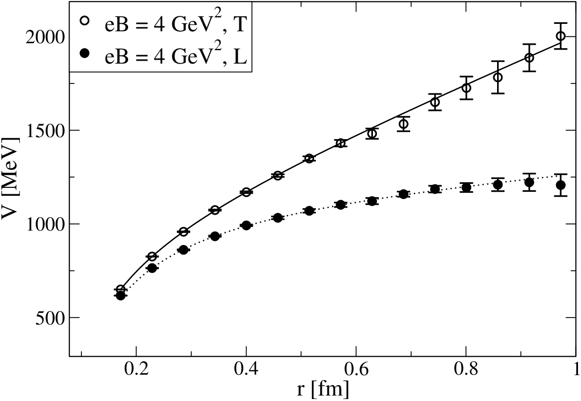
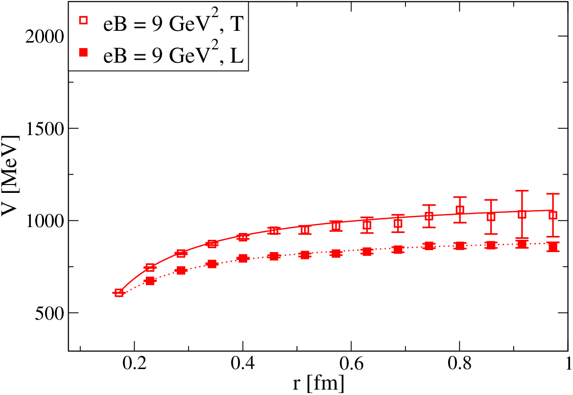
Results for the static quark-antiquark potential, computed for the two different orientations and magnetic fields, are shown in Fig. 8: the different behavior in the two phases is particularly clear, also by eye, for the transverse direction, where the linearly rising potential suddenly flattens moving from to GeV2. In order to make a more quantitative analysis, we have tried to fit data according to the Cornell ansatz
| (16) |
obtaining the following results. For GeV2, data
are well fitted (with )
by a purely Coulombic potential both in the trasverse and in the
longitudinal direction; if one tries to include a non-zero
, the fit returns negative values (for ) or
values compatible with zero within errors (for ).
For GeV2, instead, a non-zero string tension is
clearly needed in the transverse direction, with
MeV, which is not far
from the result obtained for the same
lattice spacing in Ref. parrot,
MeV; for the longitudinal
direction a full fit to Eq. (16)
returns MeV (which is
close also in this case
to the result MeV parrot),
however one should consider that in this case reasonably good fits are
obtained also assuming a purely Coulombic potential, if enough
points are discarded at short distances.
To summarize, present evidence is compatible, within numerical uncertainties, with the transition from a strongly anisotropic confined phase to a completely deconfined phase, in which the string tension vanishes in all directions, as the critical line is crossed. Such evidence should be supported by future studies, aimed at assessing in a more precise way which string tension is vanishing or not on both sides of the transition. In this respects, several scenarios are plausible, including the possibile existence of an intermediate phase in which but , for a subset of values of and .
However, the sudden drop of the transverse string tension is a quite
clear and undoubtful phenomenon even now. In the simplest scenario,
one can assume that the critical temperature continues its
drop as a function of until it hits the ground at some critical
magnetic field . That would imply that, even at , there is
no transition to an anisotropically deconfined phase where and , but rather a sudden transition to a
completely deconfined phase. Of course, even the assumption that
hits the ground is not supported, at the present time, by any
other evidence.
IV Conclusions and Perspectives
The numerical results presented in this study update our understanding of the QCD phase diagram in an external magnetic field in a substantial way, bringing new facts and new speculations into the overall picture. The main new results are that the (pseudo)critical temperature continues its steady decrease as a function of , reaching values as a low as MeV for of the order of GeV2, and that the crossover turns into a real first order transition for large enough magnetic fields. The latter fact has been speculated for a long time: in this paper we have provided first numerical evidence based on lattice simulation of QCD with physical quark masses. Moreover, we have provided a first rough location of the critical endpoint of the first order line, with , or alternatively ).
The existence and location of this critical endpoint have many significant implications: from a phenomenological point of view, especially for the possible consequences stemming from a strong first order cosmological QCD transition, which could be observable even nowadays Witten:1984rs; Applegate:1985qt; from a theoretical point of view, for a comparison with predictions from many effective model studies Cohen:2013zja; Moreira:2021ety; Ayala:2021nhx; Avancini:2012ee; Costa:2013zca; Bandyopadhyay:2020zte; Andersen:2021lnk; Mueller:2015fka.

The new facts emerging from our investigation are reported in Fig. 9, which represents our present proposal for the QCD phase diagram. The proposal contains also some question marks, concerning open issues and speculations, that essentially regards the fate of in the large limit. A naive linear extrapolation of present determinations of in the plane would imply that vanishes for GeV2: does that really happen, and in that case would 20 GeV2 be a natural scale for QCD? Or does instead flatten for larger magnetic fields, approaching a finite value, or zero, only asymptotically?
The issue will be likely solved by future studies, and is strictly
correlated to the fate of the confining properties of
the QCD vacuum in a strong magnetic field.
Indeed, if any critical magnetic field exists at where
the confining properties of QCD get disrupted, this field likely
coincides with the critical field where hits the ground:
results from Ref. parrot indicate that such critical field,
if any, is larger than 9 GeV2, and so do the finite results
presented here. One interesting point emerging
from our study is that, as one crosses the critical line,
the string tension seems to vanish, within our present numerical
uncertainties, both in the longitudinal and in the transverse
directions: if that applies down to , then one should not
expect any anisotropic deconfinement of the QCD vacuum at
large fields, as hypothesized in Ref. strongmag1,
with the string tension vanishing only in the
longitudinal direction,
but rather a sudden quench of
in all directions at .
There is a number of relevant issues that should be refined or investigated by future studies. First of all, one should consider that our study has been performed with a compromise between the need for a fine lattice spacing, in order to allow for a large magnetic field, and the need for large spatial sizes, in order to properly study thermodynamics. The compromise, given the presently available computational resources, has revealed to be not easy at all, essentially because of the unexpectedly low temperatures reached by the critical line, which forced us to work with low aspect ratios. Even if we have shown that systematics related to the finite UV cut-off and to the finite spatial size are reasonably under control, efforts should be pursued in the future to improve on such systematics.
A more precise location of the critical endpoint could be achieved following different approaches. Since the first order transition at 9 GeV2 seems to be quite strong, one could consider lower values of and investigate how the gap in physical observables changes along the transition line, trying to extrapolate the point where it vanishes. Alternatively, one could start from the low region, trying to detect the critical behavior associated with the endpoint, which is generally expected to be in the 3D-Ising universality class.
A future line of research should be dedicated to a precise characterization of the properties and differences of the two phases along the first order transition. In this investigation we have started a preliminary characterization of the confining properties, but many other relevant physical quantities should be considered, including a determination of the latent heat along the first order line and of the transport properties conductivity; Finazzo:2016mhm in both phases.
Finally, present results, in particular those regarding the critical endpoint, should be put in the framework of a more general and multidimensional view of the QCD phase diagram, including a finite baryon chemical potential Braguta:2019yci; Szymanski:2020stb; Buividovich:2021fsa; Abramchuk:2019lso; Ayala:2015lta; Ferrer:2016osp; Skokov:2011ib, different number of light fermions Kawaguchi:2021nsa or a finite rotation Yamamoto:2013zwa; Fukushima:2018grm; Chen:2021aiq; Yamamoto:2021oys.
Acknowledgements.
We thank M. Cardinali for collaboration in the early stages of this study. Numerical simulations have been performed at the IT Center of the Pisa University and on the MARCONI and MARCONI100 machines at CINECA, based on the Project IscrB_QGPSMF and on the agreement between INFN and CINECA (under projects INF20_npqcd, INF21_npqcd). F.S. is supported by the Italian Ministry of University and Research (MUR) under grant PRIN20172LNEEZ and by INFN under GRANT73/CALAT.References
- (1) D. Kharzeev, K. Landsteiner, A. Schmitt and H. -U. Yee, Lect. Notes Phys. 871, 1 (2013).
- (2) J. O. Andersen, W. R. Naylor and A. Tranberg, Rev. Mod. Phys. 88, 025001 (2016) [arXiv:1411.7176 [hep-ph]].
- (3) V. A. Miransky and I. A. Shovkovy, Phys. Rept. 576, 1 (2015) [arXiv:1503.00732 [hep-ph]].
- (4) V. Skokov, A. Y. Illarionov and V. Toneev, Int. J. Mod. Phys. A 24, 5925 (2009) [arXiv:0907.1396 [nucl-th]].
- (5) V. Voronyuk, V. D. Toneev, W. Cassing, E. L. Bratkovskaya, V. P. Konchakovski and S. A. Voloshin, Phys. Rev. C 83, 054911 (2011) [arXiv:1103.4239 [nucl-th]].
- (6) A. Bzdak and V. Skokov, Phys. Lett. B 710, 171 (2012) [arXiv:1111.1949 [hep-ph]].
- (7) W. -T. Deng and X. -G. Huang, Phys. Rev. C 85, 044907 (2012) [arXiv:1201.5108 [nucl-th]].
- (8) K. Tuchin, Adv. High Energy Phys. 2013, 490495 (2013) [arXiv:1301.0099].
- (9) R. Holliday, R. McCarty, B. Peroutka and K. Tuchin, Nucl. Phys. A 957, 406 (2017) [arXiv:1604.04572 [hep-ph]].
- (10) R. C. Duncan and C. Thompson, Astrophys. J. 392, L9 (1992).
- (11) T. Vachaspati, Phys. Lett. B 265, 258 (1991).
- (12) D. Grasso and H. R. Rubinstein, Phys. Rept. 348, 163 (2001) [astro-ph/0009061].
- (13) M. D’Elia, S. Mukherjee and F. Sanfilippo, Phys. Rev. D 82, 051501 (2010) [arXiv:1005.5365 [hep-lat]].
- (14) E. M. Ilgenfritz, M. Kalinowski, M. Muller-Preussker, B. Petersson and A. Schreiber, Phys. Rev. D 85, 114504 (2012) doi:10.1103/PhysRevD.85.114504 [arXiv:1203.3360 [hep-lat]].
- (15) G. S. Bali, F. Bruckmann, G. Endrodi, Z. Fodor, S. D. Katz, S. Krieg, A. Schafer and K. K. Szabo, JHEP 1202, 044 (2012) [arXiv:1111.4956 [hep-lat]].
- (16) V. G. Bornyakov, P. V. Buividovich, N. Cundy, O. A. Kochetkov and A. Schäfer, Phys. Rev. D 90, no.3, 034501 (2014) doi:10.1103/PhysRevD.90.034501 [arXiv:1312.5628 [hep-lat]].
- (17) H. T. Ding, C. Schmidt, A. Tomiya and X. D. Wang, Phys. Rev. D 102, no.5, 054505 (2020) [arXiv:2006.13422 [hep-lat]].
- (18) M. D’Elia, F. Manigrasso, F. Negro and F. Sanfilippo, Phys. Rev. D 98, no.5, 054509 (2018) [arXiv:1808.07008 [hep-lat]].
- (19) G. Endrodi, M. Giordano, S. D. Katz, T. G. Kovács and F. Pittler, JHEP 07, 007 (2019) [arXiv:1904.10296 [hep-lat]].
- (20) G. Endrodi, JHEP 07, 173 (2015) [arXiv:1504.08280 [hep-lat]].
- (21) E. Witten, Phys. Rev. D 30, 272-285 (1984).
- (22) J. H. Applegate and C. J. Hogan, Phys. Rev. D 31, 3037-3045 (1985)
- (23) M. D’Elia, L. Maio, F. Sanfilippo and A. Stanzione, [arXiv:2109.07456 [hep-lat]].
- (24) P. Weisz, Nucl. Phys. B 212, 1 (1983).
- (25) G. Curci, P. Menotti and G. Paffuti, Phys. Lett. B 130, 205 (1983) [Erratum-ibid. B 135, 516 (1984)].
- (26) J. Kogut and L. Susskind, Phys. Rev. D 11, 395 (1975).
- (27) C. Morningstar and M. J. Peardon, Phys. Rev. D 69, 054501 (2004) [hep-lat/0311018].
- (28) Y. Aoki, S. Borsanyi, S. Durr, Z. Fodor, S. D. Katz, S. Krieg and K. K. Szabo, JHEP 0906, 088 (2009) [arXiv:0903.4155 [hep-lat]].
- (29) S. Borsanyi, G. Endrodi, Z. Fodor, A. Jakovac, S. D. Katz, S. Krieg, C. Ratti and K. K. Szabo, JHEP 1011, 077 (2010) [arXiv:1007.2580 [hep-lat]].
- (30) S. Borsanyi, Z. Fodor, C. Hoelbling, S. D. Katz, S. Krieg and K. K. Szabo, Phys. Lett. B 730, 99 (2014) [arXiv:1309.5258 [hep-lat]].
- (31) G. ’t Hooft, Nucl. Phys. B 153, 141-160 (1979)
- (32) M. H. Al-Hashimi and U. J. Wiese, Ann. Phys. 324, 343 (2009) [arXiv:0807.0630 [quant-ph]].
- (33) M. D’Elia, Lect. Notes Phys. 871, 181 (2013) [arXiv:1209.0374 [hep-lat]].
- (34) G. Endrodi, Z. Fodor, S. D. Katz and K. K. Szabo, JHEP 1104, 001 (2011) [arXiv:1102.1356 [hep-lat]].
- (35) C. Bonati, E. Calore, S. Coscetti, M. D’Elia, M. Mesiti, F. Negro, S. F. Schifano, G. Silvi and R. Tripiccione Int. J. Mod. Phys. C 28, 05, 1750063 (2017) [arXiv:1701.00426[hep-lat]]
- (36) C. Bonati, E. Calore, M. D’Elia, M. Mesiti, F. Negro, F. Sanfilippo, S. F. Schifano, G. Silvi, R. Tripiccione Int. J. Mod. Phys. C 29, 01, 1850010 (2018) [arXiv:1801.01473 [hep-lat]]
- (37) H. T. Ding, S. T. Li, Q. Shi, A. Tomiya, X. D. Wang and Y. Zhang, Acta Phys. Polon. Supp. 14, 403 (2021) [arXiv:2011.04870 [hep-lat]].
- (38) V. A. Miransky and I. A. Shovkovy, Phys. Rev. D 66, 045006 (2002) [arXiv:hep-ph/0205348 [hep-ph]].
- (39) A. J. Mizher, M. N. Chernodub and E. S. Fraga, Phys. Rev. D 82, 105016 (2010) [arXiv:1004.2712 [hep-ph]].
- (40) C. Bonati, M. D’Elia and A. Rucci, Phys. Rev. D 92, no. 5, 054014 (2015) [arXiv:1506.07890 [hep-ph]].
- (41) C. Bonati, M. D’Elia, M. Mariti, M. Mesiti, F. Negro and F. Sanfilippo, Phys. Rev. D 89, 114502 (2014) [arXiv:1403.6094 [hep-lat]]
- (42) C. Bonati, M. D’Elia, M. Mariti, M. Mesiti, F. Negro, A. Rucci and F. Sanfilippo Phys. Rev. D 94, 094007 (2016) [arXiv:1607.08160 [hep-lat]]
- (43) C. Bonati, S. Calì, M. D’Elia, M. Mesiti, F. Negro, A. Rucci and F. Sanfilippo Phys. Rev. D 98, 054501 (2018) [arXiv:1807.01673 [hep-lat]].
- (44) C. Bonati, M. D’Elia, M. Mariti, M. Mesiti, F. Negro, A. Rucci and F. Sanfilippo, Phys. Rev. D 95, 074515 (2017) [arXiv:1703.00842 [hep-lat]].
- (45) T. D. Cohen and N. Yamamoto, Phys. Rev. D 89, no.5, 054029 (2014) [arXiv:1310.2234 [hep-ph]].
- (46) J. Moreira, P. Costa and T. E. Restrepo, Eur. Phys. J. A 57, no.4, 123 (2021) [arXiv:2101.12004 [hep-ph]].
- (47) A. Ayala, L. A. Hernández, M. Loewe and C. Villavicencio, Eur. Phys. J. A 57, no.7, 234 (2021) [arXiv:2104.05854 [hep-ph]].
- (48) S. S. Avancini, D. P. Menezes, M. B. Pinto and C. Providencia, Phys. Rev. D 85, 091901 (2012) [arXiv:1202.5641 [hep-ph]].
- (49) P. Costa, M. Ferreira, H. Hansen, D. P. Menezes and C. Providência, Phys. Rev. D 89, no.5, 056013 (2014) [arXiv:1307.7894 [hep-ph]].
- (50) A. Bandyopadhyay and R. L. S. Farias, Eur. Phys. J. ST 230, no.3, 719-728 (2021) [arXiv:2003.11054 [hep-ph]].
- (51) J. O. Andersen, Eur. Phys. J. A 57, no.6, 189 (2021) [arXiv:2102.13165 [hep-ph]].
- (52) N. Mueller and J. M. Pawlowski, Phys. Rev. D 91, no.11, 116010 (2015) [arXiv:1502.08011 [hep-ph]].
- (53) N. Astrakhantsev, V. V. Braguta, M. D’Elia, A. Y. Kotov, A. A. Nikolaev and F. Sanfilippo, Phys. Rev. D 102, no.5, 054516 (2020) [arXiv:1910.08516 [hep-lat]].
- (54) S. I. Finazzo, R. Critelli, R. Rougemont and J. Noronha, Phys. Rev. D 94, no.5, 054020 (2016) [erratum: Phys. Rev. D 96, no.1, 019903 (2017)] [arXiv:1605.06061 [hep-ph]].
- (55) V. V. Braguta, M. N. Chernodub, A. Y. Kotov, A. V. Molochkov and A. A. Nikolaev, Phys. Rev. D 100, no.11, 114503 (2019) [arXiv:1909.09547 [hep-lat]].
- (56) M. Szymański, Eur. Phys. J. ST 229, no.22-23, 3387-3394 (2020)
- (57) P. V. Buividovich, D. Smith and L. von Smekal, Eur. Phys. J. A 57, no.10, 293 (2021) [arXiv:2104.10012 [hep-lat]].
- (58) R. A. Abramchuk, M. A. Andreichikov, Z. V. Khaidukov and Y. A. Simonov, Eur. Phys. J. C 79, no.12, 1040 (2019) [arXiv:1908.00800 [hep-ph]].
- (59) A. Ayala, C. A. Dominguez, L. A. Hernandez, M. Loewe and R. Zamora, Phys. Rev. D 92, no.9, 096011 (2015) [arXiv:1509.03345 [hep-ph]].
- (60) E. J. Ferrer and V. de la Incera, Eur. Phys. J. A 52, no.8, 266 (2016) [arXiv:1603.08226 [nucl-th]].
- (61) V. Skokov, Phys. Rev. D 85, 034026 (2012) [arXiv:1112.5137 [hep-ph]].
- (62) M. Kawaguchi, S. Matsuzaki and A. Tomiya, [arXiv:2102.05294 [hep-ph]].
- (63) A. Yamamoto and Y. Hirono, Phys. Rev. Lett. 111, 081601 (2013) [arXiv:1303.6292 [hep-lat]].
- (64) K. Fukushima, Prog. Part. Nucl. Phys. 107, 167-199 (2019) [arXiv:1812.08886 [hep-ph]].
- (65) H. L. Chen, X. G. Huang and J. Liao, Lect. Notes Phys. 987, 349-379 (2021) [arXiv:2108.00586 [hep-ph]].
- (66) A. Yamamoto, Eur. Phys. J. A 57, no.6, 211 (2021) [arXiv:2103.00237 [hep-lat]].