A distribution function from population genetics statistics using Stirling numbers of the first kind: Asymptotics, inversion and numerical evaluation

Swaine L. Chen Note: Infectious Diseases Translational Research Programme and Department of Medicine, Division of Infectious Diseases, Yong Loo Lin School of Medicine, National University of Singapore, Singapore 119228, Singapore & Laboratory of Bacterial Genomics, Genome Institute of Singapore, Singapore 138672, Singapore. Email: slchen@gis.a-star.edu.sg Nico M. Temme Note: IAA, 1825 BD 25, Alkmaar, The Netherlands. Former address: Centrum Wiskunde & Informatica (CWI), Science Park 123, 1098 XG Amsterdam, The Netherlands. Email: nico.temme@cwi.nl

Abstract

Stirling numbers of the first kind are common in number theory and combinatorics; through Ewen’s sampling formula, these numbers enter into the calculation of several population genetics statistics, such as Fu’s $F_{s}$ . In previous papers we have considered an asymptotic estimator for a finite sum of Stirling numbers, which enables rapid and accurate calculation of Fu’s $F_{s}$ . These sums can also be viewed as a cumulative distribution function; this formulation leads directly to an inversion problem, where, given a value for Fu’s $F_{s}$ , the goal is to solve for one of the input parameters. We solve this inversion using Newton iteration for small parameters. For large parameters we need to extend the earlier obtained asymptotic results to handle the inversion problem asymptotically. Numerical experiments are given to show the efficiency of both solving the inversion problem and the expanded estimator for the statistical quantities.

Keywords Stirling numbers of the first kind; Asymptotic analysis; Population genetics statistics; Evolutionary inference from sequence alignments; Numerical algorithms; Cumulative distribution function.

1 Introduction

In recent papers [1] and [2] we have discussed the sum

S^{\prime}_{n,m}(\theta)=\frac{1}{(\theta)_{n}}\sum_{k=m}^{n}(-1)^{n-k}S_{n}^{(k)}\theta^{k},\quad\theta>0,

(1.1)

where $S_{n}^{(k)}$ are the Stirling numbers of the first kind defined by

(\theta)_{n}=\sum_{k=0}^{n}(-1)^{n-k}S_{n}^{(k)}\theta^{k},

(1.2)

and $(\theta)_{n}$ is the Pochhammer symbol, defined by

(\theta)_{0}=1,\quad(\theta)_{n}=\theta(\theta+1)\cdots(\theta+n-1)=\frac{\Gamma(\theta+n)}{\Gamma(\theta)}.

(1.3)

The quantity $S^{\prime}_{n,m}(\theta)$ (and related quantities) is used in the calculation of several population genetics statistics. One such statistic is Fu’s $F_{s}$ ,

F_{s}=\ln\frac{S^{\prime}_{n,m}(\theta)}{1-S^{\prime}_{n,m}(\theta)},

(1.4)

which was shown to be capable of identifying the genetic changes responsible for the increased fitness of a recently expanded clone of Campylobacter jejuni that is causing an epidemic of abortion in livestock [10]. We used asymptotic approximations of the Stirling numbers derived in [8] to compute $S^{\prime}_{n,m}(\theta)$ [1]. Subsequently, we transformed the sum into a contour integral in the complex plane, and we gave a first-order approximation of this integral for large $n$ , with $0<m<n$ and $\theta>0$ [2].

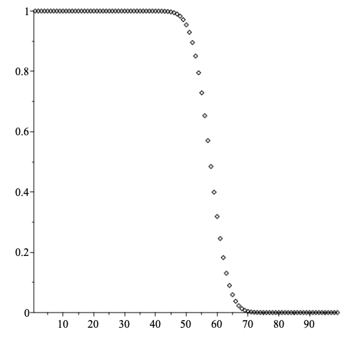
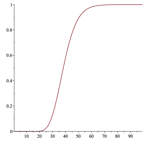
Note that, because of (1.2) the sum (1.1) satisfies $0\leq S^{\prime}_{n,m}(\theta)\leq 1$ ; see Figure 1. In fact $S^{\prime}_{n,m}(\theta)$ can be viewed as a cumulative distribution function frequently used in the derivation of several population genetics statistics, which in turn are useful for testing evolutionary hypotheses directly from DNA sequences.

In the earlier paper [2] we have derived a new integral representation of $S^{\prime}_{n,m}(\theta)$ and we have given a first-order asymptotic approximation in terms of an incomplete beta function. With these results the algorithm given in a first attempt [1] could be considerably improved in efficiency and speed.

In the present paper the main interest is the inversion problem to find $\theta$ from the equation $S^{\prime}_{n,m}(\theta)=s$ with given $s\in(0,1)$ , $n$ and $m$ . For small or intermediate values of $n$ we use a Newton iteration scheme, whereas for large $n$ we derive more details on the earlier derived asymptotic representation of $S^{\prime}_{n,m}(\theta)$ to develop an asymptotic expansion of the wanted $\theta$ . Numerical experiments are given to show the efficiency of the asymptotic expansion, of the Newton iterations, and the asymptotic inversion problem.

Refer to caption — Figure 1: Left: The function $S^{\prime}_{n,m}(\theta)$ for $m=0,1,2,\ldots,100$ ; $\theta=50$ and $n=100$ . Right: The function $S^{\prime}_{n,m}(\theta)$ for $\theta\in[0,100]$ ; $m=50$ and $n=100$ .

2 A few details on the Stirling numbers

For a concise overview of properties, of these Stirling numbers, with a summary of their uniform approximations, see [4, §11.3].

In Figure 1 we show two graphs of $S^{\prime}_{n,m}(\theta)$ , on the left left a point plot for $0\leq m\leq n$ , with fixed $\theta=50$ and $n=100$ , and on the right a smooth sigmoid curve for $0\leq\theta\leq n$ with fixed $m=50$ and $n=100$ .

A key representations for the considered asymptotic problem is the Cauchy-type integral in the complex plane

(-1)^{n-k}S_{n}^{(k)}=\frac{1}{2\pi i}\int_{{{\cal C}}}\frac{(z)_{n}}{z^{k+1}}\,dz,

(2.1)

which follows from (1.2). Here ${{\cal C}}$ is a contour around the origin.

Special values are

S_{n}^{(n)}=1\ (n\geq 0),\quad S_{n}^{(0)}=0\ (n\geq 1),\quad S_{n}^{(1)}=(-1)^{n-1}(n-1)!\ (n\geq 1),

(2.2)

and there is a recurrence relation:

S_{n+1}^{(k)}=S_{n}^{(k-1)}-nS_{n}^{(k)}.

(2.3)

For the sums $S^{\prime}_{n,m}(\theta)$ we have a new similar result.

Theorem 2.1.

The sums $S^{\prime}_{n,m}(\theta)$ satisfy for $n=2,3,4,\ldots$ the recursion

\begin{array}[]{r@{\,}c@{\,}l}(\theta+n)S^{\prime}_{n+1,m}(\theta)&=&nS^{\prime}_{n,m}(\theta)+\theta S^{\prime}_{n,m-1}(\theta),\quad 1\leq m\leq n,\\[8.0pt] S^{\prime}_{n+1,n+1}(\theta)&=&\displaystyle{\frac{\theta^{n+1}}{(\theta)_{n+1}},}\end{array}

(2.4)

with initial values

\begin{array}[]{r@{\,}c@{\,}l}S^{\prime}_{0,0}(\theta)&=&1,\quad S^{\prime}_{1,0}(\theta)=1,\quad S^{\prime}_{1,1}(\theta)=1,\\[8.0pt] S^{\prime}_{2,0}(\theta)&=&1,\quad S^{\prime}_{2,1}(\theta)=1,\quad\displaystyle{S^{\prime}_{2,2}(\theta)=\frac{\theta}{\theta+1}.}\\[8.0pt] \end{array}

(2.5)

Proof.

The proof simply follows from using the relation in (2.3). We also need $S_{n}^{(n)}=1$ and $(\theta)_{n+1}=(\theta+n)(\theta)_{n}$ . ∎

Observe that there are no Stirling numbers in the recursion in (2.4), apart from those needed to compute the starting values in (2.5). This gives a very simple method to compute $S^{\prime}_{n,m}(\theta)$ for small or intermediate values of $n$ . For large values of $n$ we prefer asymptotic representations.

The Stirling numbers are very large for large values of $n$ and $m\ll n$ , see the value of $S_{n}^{(1)}$ in (2.2). This makes straightforward evaluation of the sum in (1.1) sensitive to overflow. This problem does not happen for the recursion in (2.4), because $0\leq S^{\prime}_{n,m}(\theta)\leq 1$ .

In the initial values we see that $S^{\prime}_{n,0}(\theta)=S^{\prime}_{n,1}(\theta)=1$ for $n=0,1$ . More generally this follows from $S^{(0)}_{n}=0$ if $n\geq 1$ .

In the computation of cumulative distribution functions, like the classical gamma and beta cases, it is essential to consider the complementary relations. In the present case we use the complementary sum

T^{\prime}_{n,m}(\theta)=1-S^{\prime}_{n,m}(\theta)=\frac{1}{(\theta)_{n}}\sum_{k=0}^{m-1}(-1)^{n-k}S_{n}^{(k)}\theta^{k}.

(2.6)

To avoid numerical cancellation when using the complementary relation, we should compute first the primary function, that is, $\min(S^{\prime}_{n,m}(\theta),T^{\prime}_{n,m}(\theta))$ , and the other one from the complementary relation. The functions $T^{\prime}_{n,m}(\theta)$ satisfy the same recursion as $S^{\prime}_{n,m}(\theta)$ in (2.4), of course with different starting values.

As mentioned above, Fu’s $F_{s}$ in (1.4) is of interest for population genetics applications [3]. From (2.6), we also have a complementary equation for Fu’s $F_{s}$ ,

F_{s}=\ln\frac{1-T^{\prime}_{n,m}(\theta)}{T^{\prime}_{n,m}(\theta)}.

(2.7)

Fu’s $F_{s}$ ranges from $-\infty$ to $+\infty$ as $\theta$ runs through the interval $(0,\infty)$ and it vanishes when $\theta$ equals its transition value $\theta_{t}$ for which value we have

S^{\prime}_{n,m}(\theta_{t})=T^{\prime}_{n,m}(\theta_{t})=\tfrac{1}{2}.

(2.8)

Both representations of $F_{s}$ are needed in numerical computations, because when $S^{\prime}_{n,m}(\theta)$ is close to 1, the form with $T^{\prime}_{n,m}(\theta)$ in (2.7) gives a more reliable computational representation.

3 Summary of earlier results

Because it is more convenient to work with $S^{\prime}_{n+1,m+1}(\theta)$ we proceed with

\begin{array}[]{r@{\,}c@{\,}l}S_{n+1,m+1}(\theta)&=&\displaystyle{\frac{1}{(\theta+1)_{n}}\sum_{k=m}^{n}(-1)^{n-k}S_{n+1}^{(k+1)}\theta^{k},}\\[8.0pt] T_{n+1,m+1}(\theta)&=&\displaystyle{\frac{1}{(\theta+1)_{n}}\sum_{k=0}^{m-1}(-1)^{n-k}S_{n+1}^{(k+1)}\theta^{k}.}\end{array}

(3.1)

The following result of our paper [2] is crucial for deriving asymptotic expansions of the statistical quantities.

Theorem 3.1.

Let ${{\cal C}}_{\rho}$ be a circle at the origin of the complex plane with radius $\rho>0$ . Then $S_{n+1,m+1}^{\prime}(\theta)$ and $T_{n+1,m+1}^{\prime}(\theta)$ have representations as contour integrals

\begin{array}[]{r@{\,}c@{\,}l}S_{n+1,m+1}^{\prime}(\theta)&=&\displaystyle{\frac{\theta^{m}}{(\theta+1)_{n}}\frac{1}{2\pi i}\int_{{{\cal C}}_{\rho}}\frac{(z+1)_{n}}{z^{m}}\,\frac{dz}{z-\theta},\quad\rho>\theta,}\\[8.0pt] T_{n+1,m+1}^{\prime}(\theta)&=&\displaystyle{\frac{\theta^{m}}{(\theta+1)_{n}}\frac{1}{2\pi i}\int_{{{\cal C}}_{\rho}}\frac{(z+1)_{n}}{z^{m}}\,\frac{dz}{\theta-z},\quad\rho<\theta.}\end{array}

(3.2)

Here, $n$ and $m$ are positive integers, $0\leq m\leq n$ , and $\theta$ is a real positive number. The symbol $(\alpha)_{n}$ denotes the Pochhammer symbol introduced in (1.3).

The main asymptotic results follow from representations given in [2] and are summarised in the next theorem.

Theorem 3.2.

$S_{n+1,m+1}^{\prime}(\theta)$ and $T_{n+1,m+1}^{\prime}(\theta)$ have the representations

		$\displaystyle S_{n+1,m+1}^{\prime}(\theta)=I_{x}(m,n-m+1)+R_{n+1,m+1}^{\prime}(\theta),\quad$	$\displaystyle x={\frac{\tau}{1+\tau}},$		(3.3)
		$\displaystyle T_{n+1,m+1}^{\prime}(\theta)=I_{1-x}(n-m+1,m)-R_{n+1,m+1}^{\prime}(\theta),\quad$	$\displaystyle 1-x={\frac{1}{1+\tau}},$		(3.3)

where $I_{x}(p,q)$ is the incomplete beta function defined by

I_{x}(p,q)=\frac{1}{B(p,q)}\int_{0}^{x}t^{p-1}(1-t)^{q-1}\,dt,

(3.4)

with

0<x<1,\quad p>0,\quad q>0,\quad B(p,q)=\frac{\Gamma(p)\Gamma(q)}{\Gamma(p+q)}.

(3.5)

The term $R_{n+1,m+1}^{\prime}(\theta)$ can be expanded in negative powers of the large parameter $n$ , as will be explained in later sections. For the relation between $\tau$ and $\theta$ we refer to Definition 3.4.

Observe that in the representations given in this theorem the complementary relation in (2.6) is preserved because of the complementary property of the incomplete beta function:

I_{x}(p,q)=1-I_{1-x}(q,p).

(3.6)

3.1 The asymptotic approach

The representations given in Theorem 3.2 are obtained in [2] by using the saddle point method. The first step is the introduction of a phase function $\phi(z)$ . We write

S_{n+1,m+1}^{\prime}(\theta)=\frac{e^{-\phi(\theta)}}{2\pi i}\int_{{{\cal C}}_{\rho}}e^{\phi(z)}\,\frac{dz}{z-\theta},\quad\rho>\theta,

(3.7)

where ${{{\cal C}}_{\rho}}$ is a circle as in Theorem 3.1 and

	$\displaystyle\phi(z)$	$\displaystyle=\ln\left((z+1)_{n}\right)-m\ln z=\sum_{k=0}^{n-1}\ln(z+1+k)-m\ln z$		(3.8)
		$\displaystyle=\ln\Gamma(z+1+n)-\ln\Gamma(z+1)-m\ln z.$		(3.8)

For positive values of $z$ , we have the limiting forms

\phi(z)\sim-m\ln z,\quad z\to 0;\quad\quad\phi(z)\sim n\ln(z+1),\quad z\to\infty,

(3.9)

where the second estimate comes from $\Gamma(z+1+n)/\Gamma(z+1)\sim(z+1)^{n}$ . In addition, there is one positive minimum $z_{0}$ of $\phi(z)$ . A proof is given in [8].

The function

\chi(t)=n\ln(t+1)-m\ln t,\quad t>0,

(3.10)

has the same limiting behaviour as $\phi(z)$ at $t=0$ and as $t\to\infty$ , and it has one positive minimum $t_{0}=m/(n-m)$ . In fact, these functions behave quite similar for positive values of their arguments, and we have the following lemma.

Lemma 3.3.

Consider for positive $z$ and $t$ the equation

\phi(z)-\phi(z_{0})=\chi(t)-\chi(t_{0}).

(3.11)

Then there is a one-to-one relation between $z$ and $t$ when we use the following condition: ${\rm sign}(z-z_{0})={\rm sign}(t-t_{0})$ .

Proof.

In Figure 1 of [2] we have drawn graphs of both functions for $m=38$ and $n=100$ . Both derivaties of the non-negative convex functions have a unique positive zero $z_{0}$ and $t_{0}$ and their convex curves touch the positive real axis at $z_{0}$ and $t_{0}$ . The sign condition for the relation in (3.11) means that the left branches of the curves correspond with functions values for $z\in(0,z_{0}]$ and $t\in(0,t_{0}]$ , and the right branches with values for $z\in[z_{0},\infty)$ and $t\in[t_{0},\infty)$ . Clearly, we can uniquely determine $z(t)$ and $t(z)$ for positive values of these parameters.

∎

Before we start with deriving the asymptotic representations given in Theorem 3.2 we define the following special points used in this paper.

Definition 3.4.

Special points

The point $z_{0}$ , the positive minimum of $\phi(z)$ and the positive solution of the equation $\phi^{\prime}(z)=0$ , where

	$\displaystyle\phi^{\prime}(z)$	$\displaystyle=\sum_{k=0}^{n-1}\frac{1}{z+1+k}-\frac{m}{z}$		(3.12)
		$\displaystyle=\psi(z+n+1)-\psi(z+1)-\frac{m}{z},\quad\psi(z)=\frac{\Gamma^{\prime}(z)}{\Gamma(z)},$		(3.12)

is called the saddle point of the integral in (3.7).

2.

The value $\theta_{t}$ for which $S^{\prime}_{n,m}(\theta_{t})=T^{\prime}_{n,m}(\theta_{t})=\frac{1}{2}$ is called the transition point of $S^{\prime}_{n,m}(\theta)$ and $T^{\prime}_{n,m}(\theta)$ .
3.

The positive value of $t$ that satisfies the relation in (3.11) when $z$ is replaced by $\theta$ is called $\tau$ . That is, when we write the general solution of (3.11) as $t(z)$ , then $\tau=t(\theta)$ . Also, $\tau$ is the positive solution of

$\phi(\theta)-\phi(z_{0})=\chi(\tau)-\chi(t_{0}),\quad{\rm sign}(\theta-z_{0})={\rm sign}(\tau-t_{0}).$ (3.13)

The relation in (3.11) will be used as a transformation of variables (which is also used in [8]) and (3.7) becomes

	$\displaystyle S_{n+1,m+1}^{\prime}(\theta)$	$\displaystyle=\frac{e^{-\chi(\tau)}}{2\pi i}\int_{{\cal C}_{\sigma}}\frac{(t+1)^{n}}{t^{m}}f(t)\,dt,$		(3.14)
	$\displaystyle f(t)$	$\displaystyle=\frac{1}{z-\theta}\frac{dz}{dt},\quad\frac{dz}{dt}=\frac{\chi^{\prime}(t)}{\phi^{\prime}(z)},\quad\chi^{\prime}(t)=(n-m)\frac{t-t_{0}}{t(1+t)},$		(3.14)

with $t_{0}=m/(n-m)$ , where we have used the relation for $\chi(\tau)$ in (3.13). The value $z=\theta$ (a pole of the integrand in (3.7)) corresponds with $t=\tau$ (see Definition 3.4), and this means that the function $f(t)$ will have a pole at $t=\tau$ .

The main asymptotic result of [2] is given in the following theorem.

Theorem 3.5.

Let the function $g(t)$ be defined by

g(t)=f(t)-\frac{1}{t-\tau},

(3.15)

where $f(t)$ is defined in (3.14). Then the function $R_{n+1,m+1}^{\prime}(\theta)$ of the representations given in (3.3), has the integral representation

R_{n+1,m+1}^{\prime}(\theta)=\frac{e^{-\chi(\tau)}}{2\pi i}\int_{{\cal C}_{\sigma}}\frac{(t+1)^{n}}{t^{m}}g(t)\,dt,

(3.16)

where ${{\cal C}}_{\sigma}$ is a contour around the origin and inside the domain where $g(t)$ is analytic. A first-order approximation is given by

R_{n+1,m+1}^{\prime}(\theta)\sim e^{-\chi(\tau)}\binom{n}{m-1}\ g(t_{0}),\quad t_{0}=\frac{m}{n-m},

(3.17)

where

g(t_{0})=f(t_{0})-\frac{1}{t_{0}-\tau},\quad f(t_{0})=\frac{1}{z_{0}-\theta}\sqrt{\frac{\chi^{(2)}(t_{0})}{\phi^{(2)}(z_{0})}}.

(3.18)

The incomplete beta function (see (3.4)) is used with the representation

I_{\frac{\tau}{1+\tau}}(m,n-m+1)=\frac{e^{-\chi(\tau)}}{2\pi i}\int_{{\cal C}_{\sigma}}\frac{(t+1)^{n}}{t^{m}}\,\frac{dt}{t-\tau}.

(3.19)

This function has the representation (see [6, §8.17(i)])

I_{\frac{\tau}{1+\tau}}(m,n-m+1)=(1+\tau)^{-n}\sum_{j=m}^{n}\binom{n}{j}\tau^{j},

(3.20)

and from the complementary relation in (3.6) it follows that $I_{\frac{1}{1+\tau}}(n-m+1,m)$ used in (3.3) has the expansion

I_{\frac{1}{1+\tau}}(n-m+1,m)=(1+\tau)^{-n}\sum_{j=0}^{m-1}\binom{n}{j}\tau^{j}.

(3.21)

Remark 3.6.

The role of the transition point $\theta_{t}$ in connection with Fu’s $F_{s}$ is explained before (2.8). The transition value $\theta_{t}$ can be obtained by using the inversion methods of §4. On the other hand, the main term in the first line of (3.3) is the incomplete beta function, which function has [5] the transition point $x_{t}$ close to $x=p/(p+q)$ , which gives $\tau=m/(n+m+1)$ . This point is close to $t_{0}=m/(n+m)$ , the zero of $\chi^{\prime}(t)$ , see (3.14) and saddle point of the integral in (3.14), which corresponds to $z_{0}$ , the saddle point of integral in (3.7). We conclude that the saddle point $z_{0}$ is a good approximation of the transition value $\theta_{t}$ .

4 The inversion problem

We consider the following inversion problem: let $m$ and $n$ be given, together with a value $s\in(0,1)$ . Then find $\theta$ such that

S_{n,m}^{\prime}(\theta)=s.

(4.1)

Since $S_{n,m}^{\prime}(0)=0$ and $S_{n,m}^{\prime}(\theta)\to 1$ as $\theta\to\infty$ , and $S_{n,m}^{\prime}(\theta)$ is an increasing function of $\theta$ (see also Figure 1 (Right), there is a unique solution $\theta$ of this problem.

We consider two approaches to solve this problem, in the first one we use Newton iteration and the other one is especially useful when the parameters $n$ and $m$ are large enough to use asymptotic approximations.

In both methods we use a starting value $\theta_{0}$ that follows from the value $x$ that solves the reduced equation

I_{x}(p,q)=s,\quad p=m,\quad q=n-m+1,\quad x=\frac{\tau}{1+\tau},

(4.2)

where $I_{x}(p,q)$ is the incomplete beta function used in (3.3). With this value $x$ we compute $\tau=x/(1-x)$ and the initial value $\theta_{0}$ in the Newton method then follows from the relation between $\tau$ and $\theta$ as explained in Definition 3.4. We use the reduced equation because we consider the incomplete beta function as the main asymptotic approximant of $S_{n+1,m+1}^{\prime}(\theta)$ . Also for small values of $n$ and $m$ it gives a useful initial value $\theta_{0}$ .

The inversion of the incomplete beta function is extensively considered in the literature. For an approach for large variable $p$ and $q$ , see [7] while in [5] a fourth order fixed point method and several other approaches are discussed. For an overview of the inversion of other classical cumulative distribution functions, we refer to [9, Chapter 42].

Remark 4.1.

The inversion $S_{n,m}^{\prime}(\theta)=s$ can be replaced by the equation for the complementary function: $T_{n,m}^{\prime}(\theta)=1-s$ , which is relevant when $s\sim 1$ , and even more relevant when $s=1-\sigma$ , when $\sigma$ is known in detail as a small positive number.

Remark 4.2.

The inversion of Fu’s $F_{s}$ (see(1.4)), that is, solving the equation $F_{s}=f$ , $f\in\mathbb{R}$ , follows immediately from our methods for solving $S_{n,m}^{\prime}(\theta)=s$ . The equation $F_{s}=f$ is equivalent with solving

S_{n,m}^{\prime}(\theta)=\frac{e^{f}}{1+e^{f}},\quad T_{n,m}^{\prime}(\theta)=\frac{1}{1+e^{f}}.

(4.3)

When $f$ is a large positive number, it is very relevant to solve the second equation.

4.1 The iterative inversion method

When solving the equation in (4.1) with the Newton iterative method we compute a sequence of vales $\theta_{j}$ , $j=0,1,\ldots$ , from the scheme

\theta_{j+1}=\theta_{j}-\frac{f(\theta_{j})-s}{f^{\prime}(\theta_{j})},\quad j=0,1,2,\ldots,\quad f(\theta)=S_{n,m}^{\prime}(\theta).

(4.4)

The starting value $\theta_{0}$ is obtained from the reduced equation in (4.2). The derivative of $S_{n,m}^{\prime}(\theta)$ follows from the following lemma.

Theorem 4.3.

\frac{d}{d\theta}S_{n,m}^{\prime}(\theta)=-S_{n,m}^{\prime}(\theta)\sum_{k=0}^{n-1}\frac{1}{k+\theta}+\widehat{S}_{n,m}^{\prime}(\theta),

(4.5)

where

\widehat{S}_{n,m}^{\prime}(\theta)=\frac{1}{(\theta)_{n}}\sum_{k=m}^{n}(-1)^{n-k}kS_{n}^{(k)}\theta^{k-1}.

(4.6)

These functions satisfy the recurrence relation

(\theta+n)\widehat{S}^{\prime}_{n+1,m}(\theta)=n\widehat{S}^{\prime}_{n,m}(\theta)+\theta\widehat{S}^{\prime}_{n,m-1}(\theta)+S^{\prime}_{n,m-1}(\theta),\quad 1\leq m\leq n.

(4.7)

Proof.

First we have

\frac{d}{d\theta}\frac{1}{(\theta)_{n}}=\frac{d}{d\theta}\frac{\Gamma(\theta)}{\Gamma(\theta+n)}=\frac{\Gamma^{\prime}(\theta)}{\Gamma(\theta+n)}-\frac{\Gamma(\theta)\Gamma^{\prime}(\theta+n)}{\Gamma^{2}(\theta+n)}.

(4.8)

Next we use the $\psi$ -function, defied by $\psi(z)=\Gamma^{\prime}(z)/\Gamma(z)$ , which has the recursive property (which is also used in (3.12))

\psi(z+n)=\psi(z)+\sum_{k=0}^{n-1}\frac{1}{k+z},\quad n=1,2,3,\ldots.

(4.9)

This recursion easily follows from the fundamental property of the gamma function $\Gamma(z+1)=z\Gamma(z)$ . We find

\frac{d}{d\theta}\frac{1}{(\theta)_{n}}=\left(\psi(\theta)-\psi(\theta+n)\right)\frac{1}{(\theta)_{n}}.

(4.10)

Combining these results we find the relation in (4.5). The proof of the recurrence relation in (4.7) follows from the recurrence relation of the Stirling numbers in (2.3), just as in the proof of Theorem 2.1. ∎

A few first values of $\widehat{S}^{\prime}_{n,m}(\theta)$ are

\begin{array}[]{r@{\,}c@{\,}l}\widehat{S}^{\prime}_{0,0}(\theta)&=&0,\quad\widehat{S}^{\prime}_{1,0}=\displaystyle{\frac{1}{\theta}},\quad\widehat{S}^{\prime}_{1,1}=\displaystyle{\frac{1}{\theta}},\\[8.0pt] \widehat{S}^{\prime}_{2,0}(\theta)&=&\displaystyle{\frac{2\theta+1}{\theta(\theta+1)}},\quad\widehat{S}^{\prime}_{2,1}=\displaystyle{\frac{2\theta+1}{\theta(\theta+1)}},\quad\displaystyle{\widehat{S}^{\prime}_{2,2}=\frac{2}{\theta+1}.}\end{array}

(4.11)

In §4.3 we give numerical examples of the Newton iteration scheme.

4.2 The asymptotic inversion method

We consider the inversion of the full equation (4.1) with the representation of $S_{n+1,m+1}^{\prime}(\theta)$ as given in (3.3). We concentrate on finding $\tau$ and with this information we compute $\theta$ ; see Definition 3.4. We propose the following

Proposition 4.4.

Let $x$ be the solution of the reduced equation in (4.2), with corresponding $\tau$ value $\tau_{0}=x/(1-x)$ . Then we will construct an expansion of the wanted value $\tau$ of the form

\tau=\tau_{0}+{\varepsilon},\quad{\varepsilon}\sim\frac{\tau_{1}}{\nu}+\frac{\tau_{2}}{\nu^{2}}+\ldots,\quad\nu=n-m,

(4.12)

with

\tau_{1}=\frac{\tau_{0}(\tau_{0}+1)}{\tau_{0}-t_{0}}\ln\bigl((t_{0}-\tau_{0})f(t_{0})\bigr),

(4.13)

where $f(t_{0})$ is given in (3.18), and

\begin{array}[]{r@{\,}c@{\,}l}e^{-\xi}\tau_{2}&=&\displaystyle{\tau_{1}\frac{e^{-\xi}-1}{\xi}+\frac{(2\tau_{0}+1)\tau_{1}^{2}}{\tau_{0}(\tau_{0}+1)}\frac{e^{-\xi}-1+\xi}{\xi^{2}}\ +}\\[8.0pt] &&\displaystyle{\rho^{\prime}(\tau_{0})\tau_{1}^{3}\frac{e^{-\xi}-1+\xi-\frac{1}{2}\xi^{2}}{\xi^{3}}\ -}\\[8.0pt] &&\displaystyle{\tau_{0}(\tau_{0}+1)\left(G_{1}(t_{0})+\tau_{1}G_{0}^{\prime}(t_{0})+\tfrac{1}{2}\rho^{\prime}(\tau_{0})\tau_{1}^{2}G_{0}(t_{0})\right).}\end{array}

(4.14)

The coefficients $G_{k}(t)$ are defined in Theorem 5.1 (see also §5) and

\rho(\tau)=\frac{t_{0}-\tau}{\tau(1+\tau)},\quad\xi=\tau_{1}\rho(\tau_{0}).

(4.15)

To obtain these coefficients $\tau_{j}$ we have used a perturbation method that starts with writing $S_{n+1,m+1}^{\prime}(\theta)$ of Theorem 3.2 in the form

I_{\frac{\tau_{0}+{\varepsilon}}{1+\tau_{0}+{\varepsilon}}}(p,q)+e^{-\chi(\tau_{0}+{\varepsilon})}\binom{n}{m-1}S(\tau_{0}+{\varepsilon})=s,

(4.16)

where $S(\tau)$ is the function with expansion (see (5.1) and (3.3))

S(\tau)\sim\sum_{k=0}^{\infty}\frac{G_{k}(t_{0})}{\nu^{k}}.

(4.17)

The idea is to use the expansion of ${\varepsilon}$ given in (4.12) in (4.16), and expand the relevant terms in negative powers of $\nu$ . The coefficients of the same powers of $\nu$ in this collection should vanish. This yields equations for the coefficients $\tau_{j}$ . Because we already calculated $\tau_{0}$ such that $I_{\frac{\tau_{0}}{1+\tau_{0}}}(p,q)=s$ , we have the asymptotic equality

\sum_{k=1}^{\infty}\frac{{\varepsilon}^{k}}{k!}\frac{d^{k}}{d\tau^{k}}I_{\frac{\tau}{1+\tau}}(p,q)+\binom{n}{m-1}\sum_{k=0}^{\infty}\frac{{\varepsilon}^{k}}{k!}\frac{d^{k}}{d\tau^{k}}\left(e^{-\chi(\tau)}S(\tau)\right)=0,

(4.18)

where the derivatives are evaluated at $\tau=\tau_{0}$ . The construction of the coefficients $\tau_{j}$ can be done with the help of symbolic calculations. The technical details of the manipulations to find (4.13) and (4.14) are available from the authors.

Example 4.5.

We take $n=99$ , $m=49$ and try to find the value $\theta$ such that $S_{100,50}^{\prime}(\theta)=\frac{1}{2}$ . This means, we try to find the transition value $\theta_{t}$ for these $m$ and $n$ ; see Definition 3.4. This example corresponds with the second line in Table 2. For the asymptotic method we have the following steps.

1.

Compute the saddle point $z_{0}\doteq 39.1327$ by solving the equation $\phi^{\prime}(z)=0$ , see (3.12), and $t_{0}=49/50=0.98$ from $\chi^{\prime}(t)=0$ , see (3.14).
2.

Compute $\phi(z_{0})\doteq 259.198$ and $\chi(t_{0})\doteq 68.6165$ .
3.

With $s=\frac{1}{2}$ solve the equation $I_{x}(p,q)=\frac{1}{2}$ , see (4.2). We find $x\doteq 0.4899330675$ . This gives $\tau_{0}=x/(1-x)\doteq 0.960527$ and $\chi(\tau_{0})\doteq 68.6215$ .
4.

Use (3.13) to compute $\theta$ from the equation $\phi(\theta)=\phi(z_{0})+\chi(\tau_{0})-\chi(t_{0})\doteq 259.203$ in the interval $0,z_{0})$ (because $\tau_{0}<t_{0}$ , and find $\theta\doteq 38.29722$ .
5.

A first check: compute $S_{100,50}^{\prime}(\theta)$ with this value of $\theta$ and find $0.50233$ , with relative error $0.0047$ .
6.

Next compute $\tau_{1}$ from (4.13), with the just found value of $\theta$ that is needed in $f_{0}=f(t_{0})$ given in (3.18). Find $\tau_{1}\doteq-0.055873923$ and compute $\tau\sim\tau_{0}+\tau_{1}/\nu\doteq 0.959409535$ , with $\nu=n-m$ .
7.

Repeat the steps given above: the equation for the new $\theta$ becomes $\phi(\theta)=\phi(z_{0})+\chi(\tau_{0}+\tau_{1}/\nu)-\chi(t_{0})\doteq 259.203352$ and find $\theta\doteq 38.2492993$ .
8.

Check: compute $S_{100,50}^{\prime}(\theta)$ with this $\theta$ and find $0.5000190$ , with relative error 0.38 $e-$ 4.
9.

With the next term in the expansion, $\tau\sim\tau_{0}+\tau_{1}/\nu+\tau_{2}/\nu^{2}$ , we find $\theta\doteq 38.248908191$ , and $S_{100,50}^{\prime}(\theta)\doteq 0.500000125$ , with relative error 0.25 $e-$ 6.

Table 1: Results for inverting equation

S_{n,m}^{\prime}(\theta)=s

by using Newton iteration with starting value

\theta=\theta_{0}

and relative errors

\delta_{j}=|s/S_{n,m}^{\prime}(\theta_{j})-1|

j=0,2,4

\begin{array}[]{rccccccc}m/n&s&\theta_{0}&\delta_{0}&\theta_{2}&\delta_{2}&\theta_{4}&\delta_{4}\\ \hline\cr 10/25&0.0001&0.02&0.82&0.812&0.20e$-$00&0.78467&0.17e$-$03\\ 10/25&0.25&4.55&0.36&3.786&0.46e$-$07&3.78618&0.00e$-$00\\ 10/25&0.50&6.13&0.23&5.163&0.46e$-$03&5.16527&0.10e$-$14\\ 10/25&0.75&8.21&0.12&6.970&0.26e$-$02&6.98945&0.98e$-$10\\ 25/50&0.0001&6.20&0.64&5.70&0.46e$-$01&5.67813&0.40e$-$06\\ 25/50&0.25&16.06&0.24&14.941&0.91e$-$05&14.9416&0.10e$-$14\\ 25/50&0.50&19.70&0.15&18.373&0.18e$-$04&18.3727&0.14e$-$14\\ 25/50&0.75&24.14&0.080&22.563&0.19e$-$03&22.5663&0.10e$-$14\\ \hline\cr\end{array}

4.3 Numerical results for the inversion

In Table 1 we give the results for computing $\theta$ from the equation $S_{n,m}^{\prime}(\theta)=s$ by using Newton iteration (see §4.1). The starting value $\theta_{0}$ is obtained by inverting the reduced equation in (4.2), where also the relation between $x$ and $\theta$ is explained. In the table we give the iterated values of $\theta_{j}$ and $\delta_{j}=|s/S_{n,m}^{\prime}(\theta_{j})-1|$ for $j=0,2,4$ . As can be expected by using Newton iteration, once we have a reasonable starting value, we can obtain excellent accuracy with a few iteration steps. We even see convergence for small values $s=0.0001$ , where for the corresponding $\theta$ values the curve of $S_{n,m}^{\prime}(\theta)$ is very flat (see Figure 1, Right).

In Table 2 we give the results for computing $\theta$ by using asymptotic methods described in §4.2. The equation $S_{n+1,m+1}^{\prime}(\theta)=s$ is approximately solved by using the approximation of $\tau$ in (4.12) with terms up to $\tau_{j}$ , $j=0,1,2$ . As expected, we see a better performance when we include $\tau_{1}/\nu$ and $\tau_{1}/\nu+\tau_{2}/\nu^{2}$ .

Table 2: Results for computing

\theta

from the equation

S_{nm}^{\prime}(\theta)=s

by using the approximation of

\tau

in (4.12) with terms up to

\tau_{j}

j=0,1,2

; see (4.13) and (4.14). We give the corresponding values

\theta_{j}

and relative errors

\delta_{j}=|s/S_{nm}^{\prime}(\theta)-1|

\begin{array}[]{rccccccc}m/n&s&\theta_{0}&\delta_{0}&\theta_{1}&\delta_{1}&\theta_{2}&\delta_{2}\\ \hline\cr 200/250&0.0001&255.3&0.36e$-$2&255.339&0.24e$-$4&255.33835&0.13e$-$4\\ 200/250&0.25&408.2&0.11e$-$2&408.103&0.35e$-$5&408.10264&0.66e$-$7\\ 200/250&0.50&455.0&0.66e$-$3&454.911&0.21e$-$5&454.91098&0.18e$-$6\\ 200/250&0.75&508.2&0.34e$-$3&508.124&0.11e$-$5&508.12328&0.76e$-$8\\ 500/1000&0.0001&307.4&0.73e$-$2&307.383&0.58e$-$5&307.38266&0.32e$-$8\\ 500/1000&0.25&378.6&0.23e$-$2&378.570&0.19e$-$5&378.56980&0.10e$-$8\\ 500/1000&0.50&396.4&0.15e$-$2&396.387&0.11e$-$5&396.39298&0.20e$-$3\\ \ 500/1000&0.75&415.1&0.77e$-$3&415.025&0.62e$-$6&415.02539&0.20e$-$9\\ \hline\cr\end{array}

5 Deriving the complete asymptotic expansion

The first-term approximation in our previous result in (3.16) of Theorem 3.5 will now be extended in the following theorem.

Theorem 5.1.

Let $R_{n+1,m+1}^{\prime}(\theta)$ be defined as in (3.16). Then for $N=0,1,2,\ldots$

R_{n+1,m+1}^{\prime}(\theta)=e^{-\chi(\tau)}\binom{n}{m-1}\sum_{k=0}^{N-1}\frac{G_{k}(t_{0})}{\nu^{k}}+\frac{e^{-\chi(\tau)}}{2\pi i\nu^{N}}\int_{{\cal C}_{\sigma}}\frac{(t+1)^{n}}{t^{m}}G_{N}(t)\,dt,

(5.1)

where $\nu=n-m$ , $G_{0}(t)=g(t)$ , see (3.15), and other $G_{k}(t)$ follow from the recursive scheme

H_{k}(t)=\frac{G_{k}(t)-G_{k}(t_{0})}{t-t_{0}},\quad G_{k+1}(t)=-\frac{d}{dt}\Bigl(t(1+t)H_{k}(t)\Bigr),\quad k=0,1,2,\ldots\,.

(5.2)

Proof.

We start with the representation in (3.16) and use an integration by parts procedure, which starts by writing

G_{0}(t)=G_{0}(t_{0})+(t-t_{0})H_{0}(t),\quad G_{0}(t)=g(t).

(5.3)

This gives

R_{n+1,m+1}^{\prime}(\theta)=G_{0}(t_{0})e^{-\chi(\tau)}\binom{n}{m-1}+\frac{e^{-\chi(\tau)}}{2\pi i}\int_{{\cal C}_{\sigma}}\frac{(t-t_{0})H_{0}(t)}{\chi^{\prime}(t)}\,de^{\chi(t)},

(5.4)

and using $\chi^{\prime}(t)$ shown in (3.14), we find

R_{n+1,m+1}^{\prime}(\theta)=G_{0}(t_{0})e^{-\chi(\tau)}\binom{n}{m-1}+\frac{e^{-\chi(\tau)}}{2\pi i\nu}\int_{{\cal C}_{\sigma}}\frac{(t+1)^{n}}{t^{m}}G_{1}(t)\,dt,

(5.5)

where

G_{1}(t)=-\frac{d}{dt}\bigl(t(1+t)H_{0}(t)\bigr).

(5.6)

This integral has the same form as the one in (3.16), and we can continue this method. This proves the theorem.

∎

The first coefficients $G_{k}(t_{0})$ of the expansion in (5.1) are

\begin{array}[]{r@{\,}c@{\,}l}G_{0}(t_{0})&=&g_{0},\quad G_{1}(t_{0})=-(1+2t_{0})g_{1}-t_{0}(t_{0}+1)g_{2},\\[8.0pt] G_{2}(t_{0})&=&2(1+2t_{0})g_{1}+(2+11t_{0}+11t_{0}^{2})g_{2}\ +\\[8.0pt] &&5t_{0}(t_{0}+1)(1+2t_{0})g_{3}+3t_{0}^{2}(t_{0}+1)^{2}g_{4}.\end{array}

(5.7)

The coefficients $g_{k}$ follow from the coefficients $f_{k}$ in the expansion $\displaystyle{f(t)=\sum_{k=0}^{\infty}f_{k}(t-t_{0})^{k}}$ , with $f(t)$ defined in (3.14). We have

g(t)=f(t)-\frac{1}{t-\tau}=\sum_{k=0}^{\infty}g_{k}(t-t_{0})^{k}\quad g_{k}=f_{k}-\frac{(-1)^{k}}{(t_{0}-\tau)^{k+1}}.

(5.8)

Finally, all these coefficients can be expressed in terms of the coefficients $z_{k}$ of the expansion

z-z_{0}=\sum_{k=1}^{\infty}z_{k}(t-t_{0})^{k},

(5.9)

and these follow from substituting this expansion in the Taylor expansions of the functions used in the transformation given in (3.11). This transformation has the local expansions at the saddle points

(z-z_{0})\sqrt{\sum_{k=2}^{\infty}\frac{1}{k!}\phi^{(k)}(z_{0})(z-z_{0})^{k-2}}=(t-t_{0})\sqrt{\sum_{k=2}^{\infty}\frac{1}{k!}\chi^{(k)}(t_{0})(t-t_{0})^{k-2}},

(5.10)

where the square roots are positive for positive values of $z$ and $t$ . The derivatives $\phi^{(k)}(z)$ can be expressed in terms of the derivatives of the gamma functions; see (3.12). The derivatives $\chi^{(k)}(t)$ at $t=t_{0}$ are simple expressions.

The first coefficients $z_{k}$ are

z_{1}=\sqrt{\frac{\chi^{(2)}(t_{0})}{\phi^{(2)}(z_{0})}},\quad z_{2}=\frac{\chi^{(3)}(t_{0})-z_{1}^{3}\phi^{(3)}(z_{0})}{6z_{1}\phi^{(2)}(z_{0})}.

(5.11)

The first coefficients $f_{k}$ are

\begin{array}[]{r@{\,}c@{\,}l}f_{0}&=&\displaystyle{\frac{z_{1}}{z_{0}-\theta}},\quad f_{1}=\displaystyle{\frac{2z_{2}z_{0}-2z_{2}\theta-z_{1}^{2}}{(\theta-z_{0})^{2}}}\\[8.0pt] f_{2}&=&\displaystyle{\frac{6z_{3}z_{0}\theta+3z_{1}z_{2}z_{0}-3z_{1}z_{2}\theta-z_{1}^{3}-3z_{3}z_{0}^{2}-3z_{3}\theta^{2}}{(\theta-z_{0})^{3}}}.\end{array}

(5.12)

Then, the first coefficients $g_{k}$ follow from (5.8).

Table 3: Values of the relation (5.13) in the computation of

S^{\prime}_{n,m}(\theta)

for

n=1.000

and

n=100.000

for several values of

m

and

\theta

\begin{array}[]{ccccccc}\hline\cr n=1.000&{\rm Digits}=16&4\ {\rm terms}&&&&\\ \hline\cr\rho\ \backslash\ m&150&300&450&600&750&900\\ \hline\cr 0.70&0.16e$-$12&0.27e$-$13&0.73e$-$13&0.10e$-$12&0.12e$-$12&0.47e$-$13\\ 0.80&0.32e$-$12&0.13e$-$12&0.16e$-$12&0.86e$-$13&0.11e$-$12&0.88e$-$13\\ 0.90&0.24e$-$11&0.30e$-$12&0.70e$-$13&0.60e$-$13&0.50e$-$12&0.13e$-$10\\ 1.00&0.12e$-$11&0.19e$-$11&0.14e$-$12&0.54e$-$12&0.29e$-$11&0.79e$-$13\\ \hline\cr n=1.000&{\rm Digits}=20&4\ {\rm terms}&&&&\\ \hline\cr\rho\ \backslash\ m&150&300&450&600&750&900\\ \hline\cr 0.70&0.78e$-$15&0.58e$-$16&0.17e$-$17&0.49e$-$16&0.16e$-$16&0.24e$-$16\\ 0.80&0.47e$-$15&0.48e$-$16&0.93e$-$17&0.16e$-$16&0.60e$-$18&0.20e$-$16\\ 0.90&0.12e$-$15&0.36e$-$16&0.28e$-$16&0.60e$-$17&0.56e$-$16&0.20e$-$14\\ 1.00&0.17e$-$15&0.14e$-$15&0.93e$-$16&0.37e$-$16&0.37e$-$16&0.95e$-$16\\ \hline\cr n=100.000&{\rm Digits}=16&2\ {\rm terms}&&&&\\ \hline\cr\rho\ \backslash\ m&15.000&30.000&45.000&60.000&75.000&90.000\\ \hline\cr 0.97&0.53e$-$10&0.36e$-$10&0.86e$-$11&0.82e$-$11&0.24e$-$11&0.47e$-$11\\ 0.98&0.58e$-$11&0.12e$-$10&0.61e$-$11&0.14e$-$10&0.16e$-$11&0.17e$-$10\\ 0.99&0.86e$-$11&0.17e$-$10&0.18e$-$10&0.16e$-$10&0.20e$-$10&0.44e$-$11\\ 1.00&0.34e$-$09&0.28e$-$08&0.47e$-$09&0.14e$-$08&0.46e$-$11&0.19e$-$08\\ \hline\cr n=100.000&{\rm Digits}=20&2\ {\rm terms}&&&&\\ \hline\cr\rho\ \backslash\ m&15.000&30.000&45.000&60.000&75.000&90.000\\ \hline\cr 0.97&0.20e$-$14&0.21e$-$14&0.16e$-$14&0.16e$-$14&0.63e$-$15&0.97e$-$15\\ 0.98&0.37e$-$14&0.38e$-$14&0.15e$-$14&0.29e$-$16&0.80e$-$15&0.25e$-$15\\ 0.99&0.85e$-$14&0.10e$-$14&0.18e$-$14&0.14e$-$14&0.16e$-$14&0.64e$-$15\\ 1.00&0.71e$-$13&0.22e$-$12&0.23e$-$13&0.15e$-$13&0.18e$-$12&0.51e$-$13\\ \hline\cr\end{array}

5.1 Numerical verifications of the asymptotic approximation

A convenient tool for verifying the errors in numerical calculations is the recursion in Theorem 2.1, (2.4). We can write this in the form

\frac{nS^{\prime}_{n,m}(\theta)+\theta S^{\prime}_{n,m-1}(\theta)}{(\theta+n)S^{\prime}_{n+1,m}(\theta)}-1=0.

(5.13)

Especially for large values of $n$ (for example, $n=100.000$ ) used in the tests we avoid the exact evaluation of the sums in (1.1), and we accept that we do not verify a standard relative error.

In Table 3 we show the values of the relation (5.13) in the computation of $S^{\prime}_{n,m}(\theta)$ for $n=1000$ and $n=100.000$ for several values of $m$ . In the first two parts ( $n=1.000$ ) of the table we used the expansion in (5.1) with terms up to and including $k=3$ , and in the final two parts ( $n=100.000$ ) we only used the terms with $G_{0}(t_{0})$ and $G_{1}(t_{0})$ . We have taken $\theta=\rho z_{0}$ , for the shown values of $\rho$ . In this way the values of $S^{\prime}_{n,m}(\theta)$ are not very small. For example, with $n=1000.000,\ m=75.000,\ z_{0}\doteq 136312.21$ , we have

\begin{array}[]{ll}\rho=0.97\quad\Longrightarrow\quad S^{\prime}_{n,m}(\theta)\doteq 0.300778124649e$-$04,\\[8.0pt] \rho=1.00\quad\Longrightarrow\quad S^{\prime}_{n,m}(\theta)\doteq 0.501722781430e$-$00.\end{array}

(5.14)

The computations are done with Maple 2020, Digits=16. To show the effect of cancellation or rounding errors, we have used the same Maple codes with Digits=20.

The first three coefficients $G_{k}(t_{0})$ of the expansion in (5.1) are given in (5.7). Each $G_{k}(t_{0})$ is a linear combination of coefficients $g_{k}$ , $k=1,2,\ldots,2k$ , and these are defined in (5.8). When $\theta\sim\theta_{t}$ , the transition value, $|t_{0}-\tau|$ is small, and in the limit $\tau\to t_{0}$ the coefficient $g_{k}$ is well defined, although $f_{k}$ has a pole at $t=t_{0}$ with corresponding $z$ -value $\theta=z_{0}$ (see the definition of $f(t)$ in (3.14)). In $g_{k}$ these poles are cancelled. From an analytical point of view, everything runs fine, but the algorithm needs special attention. For this we use expansions of $g_{k}$ for small values of $|t_{0}-\tau|$ in the form

g_{k}=\sum_{j=0}^{\infty}g_{j,k}(\tau-t_{0})^{j},\quad k=0,1,2,\ldots\,.

(5.15)

The largest errors in the first part and third part (both with Digits=16) in Table 3 occur for $\rho=1$ , that is, when $\theta=z_{0}$ , hence $\theta\sim\theta_{t}$ , the transition value. In this case $\tau\sim t_{0}$ . This is related to the difficulty of computing the coefficients $G_{k}(t_{0})$ near the transition point $\theta_{t}$ , which is near $z_{0}$ , as explained in Definition 3.4 ad Remark 3.6. This is an interesting analytical issue, but for the population genetics application area it is less important. In fact we accept some loss of accuracy near the transition point instead of using more complicated analytical expansions of the coefficients.

6 Conclusions

We have provided additional details for the asymptotic approximation of the cumulative distribution quantities $S^{\prime}_{n,m}(\theta)$ and $T^{\prime}_{n,m}(\theta)=1-S^{\prime}_{n,m}(\theta)$ . As a completely new contribution, we have considered the inversion problem to compute $\theta$ , the solution of the equation $S^{\prime}_{n,m}(\theta)=s$ , with given $s\in(0,1)$ , $m$ and large $n$ . A simple inversion method uses Newton iteration, the other one asymptotic approximations. For this we provided additional coefficients in the earlier given asymptotic expansion. We have shown that some loss of accuracy is localized near the transition values. We further observe that these estimation errors can be mitigated with additional terms of the expansion. These errors are largely in a regime where the distribution functions are near the changeover value $\frac{1}{2}$ , which is an interesting domain from an analytical point of view, but where Fu’s $F_{s}$ values are not important for genetic inferences.

Acknowledgments

SLC acknowledges members of the Chen lab for fruitful discussions. NMT acknowledges the help of Edgardo Cheb-Terrab (Maplesoft) and CWI, Amsterdam for scientific support.
SLC was supported by the National Medical Research Council, Ministry of Health, Singapore (grant numbers NMRC/OFIRG/0009/2016 and
NMRC/CIRG/1467/2017).
NMT was supported by the Ministerio de Ciencia e Innovación, Spain, projects MTM2015-67142-P (MINECO/FEDER, UE) and
PGC2018-098279-B-I00 (MCIU/AEI/FEDER, UE).

References

[1] S. L. Chen. Implementation of a Stirling number estimator enables direct calculation of population genetics tests for large sequence datasets. Bioinformatics, 35(15):2668–2670, 2019.
[2] S. L. Chen and N. M. Temme. A faster and more accurate algorithm for calculating population genetics statistics requiring sums of Stirling numbers of the first kind. G3: Genes, Genomes, Genetics, 2020. https://doi.org/10.1534/g3.120.401575.
[3] Y. X. Fu. Statistical tests of neutrality of mutations against population growth, hitchhiking and background selection. Genetics, 147(2):915–925, Oct 1997.
[4] A. Gil, J. Segura, and N. M. Temme. Numerical Methods for Special Functions. Society for Industrial and Applied Mathematics (SIAM), Philadelphia, PA, 2007.
[5] A. Gil, J. Segura, and N. M. Temme. Efficient algorithms for the inversion of the cumulative central beta distribution. Numer. Algorithms, 74(1):77–91, 2017.
[6] R. B. Paris. Chapter 8, Incomplete gamma and related functions. In NIST Handbook of Mathematical Functions, pages 173–192. U.S. Dept. Commerce, Washington, DC, 2010. http://dlmf.nist.gov/8.
[7] N. M. Temme. Asymptotic inversion of the incomplete beta function. J. Comput. Appl. Math., 41(1-2):145–157, 1992.
[8] N. M. Temme. Asymptotic estimates of Stirling numbers. Stud. Appl. Math., 89(3):233–243, 1993.
[9] N. M. Temme. Asymptotic methods for integrals, volume 6 of Series in Analysis. World Scientific Publishing Co. Pte. Ltd., Hackensack, NJ, 2015.
[10] Z. Wu, B. Periaswamy, O. Sahin, M. Yaeger, P. Plummer, W. Zhai, Z. Shen, L. Dai, S. L. Chen, and Q. Zhang. Point mutations in the major outer membrane protein drive hypervirulence of a rapidly expanding clone of Campylobacter jejuni. Proc. Natl. Acad. Sci. U.S.A., 113(38):10690–10695, 09 2016.