(P)reheating Effects of the Kähler Moduli Inflation I Model
Abstract
We investigate reheating in the string-theory-motivated Kähler Moduli Inflation I (KMII) potential, coupled to a light scalar field and produce constraints and forecasts based on Cosmic Microwave Background (CMB) and gravitational wave observables. We implement a Markov Chain Monte Carlo (MCMC) sampling method to compute the adopted model’s parameter ranges allowed by the current CMB observations. Floquet analysis and numerical lattice simulations are performed to analyze the nonlinear effects of the model’s (p)reheating phase. We derive bounds on the CDM parameters , , , and based on Planck results, finding that correlations between model parameters severely constrain the range of these parameters allowed within this model. While the KMII potential’s non-vanishing minimum may provide a possible source for the observed dark energy density this cannot be tested with current observations. We estimate the CI bounds on the inflaton mass and reheating temperature to be and , respectively. We observe both self-resonance and parametric resonance instability band structures in our Floquet analysis results. Finally, we do not observe any formation of oscillon configurations in our lattice simulations; however, our results predict a stochastic gravitational wave background generated during preheating that would be observable today in the – frequency range.
I Introduction
Inflation has had immense success since its proposal Guth 1981; Linde 1982a; Linde 1982b; Albrecht and Steinhardt 1982; Linde 1983 as it provides an attractive mechanism for explaining the observed structures in the Universe, and among several others, solves the horizon and flatness problems. Current observations favor an inflationary paradigm, particularly from an almost scale-invariant spectrum of primordial curvature perturbations imprinted in both the Cosmic Microwave Background (CMB) de Bernardis et al. 2000 and large scale structure Tegmark et al. 2004; Seljak et al. 2005; Blake et al. 2011. The simplest inflationary scenario describes the period of exponential expansion being driven by the slow-roll of a scalar field known as the inflaton. At the end of inflation, it is generally assumed the inflaton coherently oscillates at the minimum of its potential, decaying and transferring its energy to a relativistic plasma. This post-inflationary process that repopulates our Universe with ordinary matter is known as reheating. Traditional treatments of reheating are based on the idea that the spatially coherent oscillations of the inflaton corresponding to a collection of zero-momentum inflaton particles lead to the production of the elementary particles Dolgov and Linde 1982; Abbott et al. 1982; Kolb and Turner 1990, which in turn interact with one another to come to a state of thermal equilibrium, recovering standard big bang cosmology.
A perturbative approach to study the effects of the reheating mechanism is viewed as inefficient. Studies have shown the post-inflationary dynamics can be driven by two types of resonance phenomena: self-resonance of the inflaton Traschen and Brandenberger 1990; Kofman et al. 1994; Shtanov et al. 1995 and parametric resonance of the spectator (or daughter) field(s). Tachyonic instability can also develop during this phase in models with spontaneous symmetry breaking. This initial period when rapid non-perturbative particle production effects usually occur is known as preheating. The stage after preheating is a period of turbulence, followed by a longer period of perturbative decay, and finally, thermalization.
For concreteness, we turn here to a theoretically-motivated class of inflation models. A popular and promising candidate for the theory of quantum gravity is string theory and its applications to cosmology have been an active research area over the last two decades (see Refs. Cline 2006; Kallosh 2008; McAllister and Silverstein 2008 for reviews). In particular, there has been significant work on the development of inflation models based on string theory Kachru et al. 2003a; Balasubramanian and Berglund 2004; Blanco-Pillado et al. 2004; Balasubramanian et al. 2005; Conlon and Quevedo 2006a; Blanco-Pillado et al. 2006; Cicoli et al. 2009. Models of modular (or moduli) inflaton are described by the inflaton living in the closed string sector. In contrast, brane inflation Dvali and Tye 1999 deals with the open string sector. Several popular examples of inflation models in string theory include the Kachru-Kallosh-Linde-Trivedi (KKLT) scenario Kachru et al. 2003a, Kachru-Kallosh-Linde-Maldacena-McAllister-Trivedi (KKLMMT) scenario Kachru et al. 2003b, and models based on the so-called Large Volume Scenario (LVS) Balasubramanian et al. 2005 such as the Kähler moduli inflation Conlon and Quevedo 2006a, and Roulette inflation Bond et al. 2007. Several other string-theory-motivated cosmological scenarios include racetrack inflation Blanco-Pillado et al. 2004; Blanco-Pillado et al. 2006, D-term inflation Binetruy and Dvali 1996; Kachru et al. 2003b, pre-big bang Gasperini and Veneziano 2016, rolling tachyon Sen 2002, string or brane gas Battefeld and Watson 2006, and ekpyrotic scenarios Khoury et al. 2001.
In this work, we consider a simplified version of the Kähler moduli inflation, referred to as the Kähler Moduli I Inflation (KMII) Conlon and Quevedo 2006a (see also Ref. Blanco-Pillado et al. 2010), which has a non-vanishing potential minimum, providing a possible source for the observed cosmological constant’s energy density . The assumption that the total vacuum energy density of the Universe is zero due to some unknown symmetry must be taken for to be sourced from the KMII potential’s minimum. The KMII model was primarily chosen because it provides one of the simplest descriptions of the physics within the context of modular inflation, and it is also one of the simplest models with a non-vanishing minimum. The potential with the field canonically normalized is known as the “Kähler Moduli II Inflation” (KMIII) model Conlon and Quevedo 2006a; Bond et al. 2007, where the potential minimum takes large positive or negative values. Note that for providing a source for , the model must be consistent with observations when the potential minimum takes the value . In most cases, this condition is not satisfied. The scenario where is sourced by the non-vanishing minimum of the inflation potential has been examined for different inflation models, e.g., Twisted Inflation Davis et al. 2010 as well as others. An uplifting term is often induced in certain string-theory-motivated inflation potentials, e.g., in the KKLT scenario Kachru et al. 2003a, to provide a positive value of potential energy that can act as .
Preheating in inflation models based on the KKLT scenario Kachru et al. 2003a and the Kähler moduli Conlon and Quevedo 2006a or Roulette Bond et al. 2007 inflation models have been studied in detail using numerical lattice simulations Barnaby et al. 2009; Antusch et al. 2018; Kasuya et al. 2020. It was found in Ref. Barnaby et al. 2009 that both tachyonic instability and broad parametric resonance occur during preheating after modular inflation, where the inflation models are specified by a Kähler potential and its superpotential. Refs. Antusch et al. 2018; Kasuya et al. 2020 extended the analysis by focusing on the production of soliton-like configurations known as oscillons in string moduli models. We turn our attention to exploring the viability, effects, and predictions of the KMII potential which may provide a possible source for with its non-vanishing minimum. The potential minimum is constrained by fixing its dimensionless free parameter that characterizes the shape of the potential. For simplicity, we consider a four-leg quadratic interaction in all our analyses.
The remainder of the article is arranged as follows: In Sec. II, we introduce the adopted model which is analyzed in detail in the later sections. The constraints on the model, including the constraints on the post-inflationary reheating era, based on the CMB observational constraints are discussed in Sec. III. In Sec. IV, we perform Floquet analysis to analyze preheating instabilities in the model due to both self- and parametric resonant effects. We further explore the preheating effects, focusing on the stochastic gravitational wave background generated during preheating, using numerical lattice simulations in Sec. V. Finally, in Sec. VI, we conclude with a summary of the results and discuss their implications. Throughout the article, we use natural units in which and the reduced Planck mass is related to the gravitational constant through .
II KMII Model
Inflationary scenarios within the framework of moduli stabilization mechanisms Balasubramanian et al. 2005, in particular, the Kähler moduli inflation scenarios Conlon and Quevedo 2006b; Blanco-Pillado et al. 2010; Lee and Nam 2011, have regained some interest in the past decade. These models generally arise from the so-called Large Volume Compactification scenarios of Type IIB string theory. One or more complex moduli can be displaced from their minimum, with the resulting potential energy driving inflation in the three-dimensional bulk. One example of string theory-motivated inflationary potentials is the KMII model Conlon and Quevedo 2006b; Martin et al. 2013. It was shown in Ref. Conlon and Quevedo 2006b that, when a large field limit is taken, the resulting inflationary potential can be simplified to
| (1) |
where is the modulus acting as inflaton field, is the energy scale, and is a positive dimensionless parameter of the model. In Kähler inflation models, is related to the overall volume of the Calabi-Yau, the values of the other (stable) moduli, and couplings that are specific to a given compactification. arises when the Lagrangian is written as a function of the modulus field before it is canonically normalized. We adopt this model for its simplicity, as the field-redefined version (KMIII) has a very similar shape but is analytically less tractable. The KMII potential is displayed in Fig. 1 where is fixed at . As shown in Ref. Martin et al. 2013, is constrained at for inflation to successfully end by slow-roll violation. The potential has a minimum at where it takes the form .

For our analyses, we adopt an inflation model consisting of the KMII directly coupled to a light scalar field , which is assumed to be short-lived and to quickly decay to radiation. A four-leg interaction Lagrangian term , being the small coupling constant, is considered. We assume for simplicity that the bare mass of the field is small such that the mass of the field is given by . This yields the full Lagrangian
| (2) |
The adopted model has three parameters: , , and . The potential minimum can be constrained to a value equivalent to by fixing to a value very close, but not equal, to . Depending on the value of , the term in the KMII model would need to be fine-tuned to about decimal places to be comparable to , which is not feasible for analyses. For this reason, we approximate the condition by setting the minimum of the KMII potential such that which leads to the potential minimum of and avoids a period of early dark energy domination. The condition is relaxed in Sec. V.1 where we study the effects of shifting the KMII potential minimum to small positive values.
III Constraints on Model Parameters
In this section, the KMII model is quantified using three slow-roll parameters which allow one to relate the model parameters to the -Cold Dark Matter (CDM) parameters constrained by CMB data. These slow-roll parameters can also be used to determine if or when inflation ends. The preliminary analysis on the model parameters was performed using the Accurate Slow-roll Predictions for Inflationary Cosmology (ASPIC) library Martin et al. 2013. A Markov Chain Monte Carlo (MCMC) Foreman-Mackey et al. 2013 sampling method, constrained by the latest 2018 release of the Planck CMB data Akrami et al. 2020, was implemented to compute the allowed ranges of the model parameters. The marginalized posterior distributions of both the model and derived CDM parameters were computed and presented here.
Sec. III.1 presents the slow-roll parameters that are used to quantify the KMII model. The expressions relating an inflation model, CDM parameters, and reheating are detailed in Sec. III.2. The derived expressions are then applied to the adopted model in Sec. III.3, and Sec. III.4 details the MCMC sampling analysis that we implemented to compute the allowed ranges of the adopted model and derived CDM parameters.
III.1 Slow-roll Analysis
Within the slow-roll approximation formalism, we consider three slow-roll parameters , , and for quantifying inflation. They are defined by
| (3) |
where , , and are the first, second, and third derivatives of with respect to . Inflation models can be constrained by the observed tensor-to-scalar power ratio (), the scalar spectral index (), and its running (). At a given pivot scale , they can be approximated as functions of the slow-roll parameters
| (4) |
and one can obtain the scalar power spectrum amplitude using
| (5) |
The slow-roll conditions , , and must be satisfied for a successful inflation phase to occur and last sufficiently long. Inflation ends when the slow roll conditions are violated: or . The three slow-roll parameters corresponding to the KMII model can be expressed as
| (6) |
where . The first expression in Eq. (6) shows that undergoes slow-roll as the field approaches its minimum from the right side of the potential (see Fig. 1). Fig. 2 displays, when (red line), the violation condition is satisfied at , and inflation terminates successfully.
Replacing in Eq. (6) by , we obtain the following expressions for the CDM parameters using Eqs. (4), (5), and (6)
| (7) | ||||
| (8) | ||||
| (9) | ||||
| (10) |
According to the latest 2018 release of the Planck CMB data Akrami et al. 2020, the constrained CDM parameter values modeled including and and based on the Planck TT+TE+EE+lowl+lowE+lensing data in combination with the BICEP2/Keck Array () Ade et al. 2018 – Planck with the pivot scale chosen at are , , , and . The constrained parameter values based on Planck in combination with and baryon acoustic oscillation () – Planck are , , , and . For preliminary analysis, we use the ASPIC library Martin et al. 2014 to compute the slow-roll predictions corresponding to the KMII potential by setting such that , and compare them against the constrained contours from Planck and Planck data. The approximate expressions for , , and used in ASPIC (see Ref. Martin et al. 2013) have different forms compared to the ones used in this work, however, both sets of expressions estimate the same results.
It is particularly important to compute the observational predictions of the KMII model in the plane for specific values of to estimate the corresponding reheating temperature () lower bounds. must be higher than the big bang nucleosynthesis (BBN) energy scale (), and the upper bound of is constrained at since higher temperatures can result in the production of unwanted relics such as gravitinos Giudice et al. 1999; Kallosh et al. 2000; Kawasaki et al. 2005. Although currently loosely constrained, has several important applications in cosmology such as the success of BBN, baryonic asymmetry, production of dark matter during reheating Garcia et al. 2020, and constraints on various dark matter scenarios Fornengo et al. 2003; Roszkowski et al. 2014; Choi and Takahashi 2017.
A preliminary lower bound on was estimated by comparing the predictions of the KMII model against the contours presented by Planck. The results are shown in Fig. 3. The figure includes the and contours ( and confidence level – CL regions) for from the Planck (red) and Planck (blue) data. The results show is consistent with both the Planck and Planck contours. The energy scale in Fig. 3 with suggests and when compared against the contours from Planck and Planck data at CL, respectively. We find that varying does not significantly affect the lower bound predictions.

III.2 Relating Inflation, CDM Parameters, and Reheating
We now turn to the full analysis where we estimate the adopted model parameter allowed ranges based on the constrained CDM parameter values from CMB data and compute the CDM posterior distributions. It was first shown in Ref. Martin and Ringeval 2010 that the reheating era parameters can be indirectly constrained using CMB data. As illustrated in Fig. 4, the reheating era can influence the CDM parameters by modifying the expansion rate of the Universe. Based on the method developed in Ref. Martin and Ringeval 2010, Ref. Cook et al. 2015 constrained the reheating era in several single-field inflation models, and Ref. Drewes et al. 2017 extended the analysis to -attractor inflation models. We derive the desired expressions following these references which we integrate into an MCMC sampling analysis (see Sec. III.4).
The reheating era is generally defined as the period between , when slow roll ends, and the equivalency of the Hubble parameter and total inflaton decay rate , which marks the beginning of the radiation domination era. However, can occur either before or after radiation domination begins depending on how the thermalization process occurs (see, e.g., Ref. Mazumdar and Zaldivar 2014 for a detailed discussion). We assume that occurs at approximately the same time when radiation domination begins for the purposes of this work. Note that here refers to the total decay rate of the inflaton to the field, which is assumed to quickly decay to radiation. A trilinear coupling term arises due to the background value of that dominates during the perturbative stage of reheating. The perturbative reheating decay rate is thereby denoted by .
Defining as the number of e-folds, the reheating period ends at
| (11) |
where , and are the scale factors at the end of inflation and reheating, respectively. is related to the energy density at the end of the reheating era through the relation
| (12) |
where is the energy density at the end of the reheating era and is the effective number of relativistic degrees of freedom at the end of reheating ( for the SM). Soon afterward, the energy density of radiation overcomes that of the inflaton, , leading to the onset of the radiation-dominated era. can therefore be interpreted as a physical temperature associated with the onset of radiation domination.
The CMB can be related to the reheating era mainly through the equation of state parameter which varies as the Universe transitions from the reheating to radiation domination era. The energy density of the Universe can be written as
| (13) |
where is the energy density at the end of inflation given by
| (14) |
The Friedmann equation during the reheating period can then be written
| (15) |
As we consider the standard definition of reheating era ending when at , with reheating approximated by a constant equation of state , Eq. (15) can be used to express
| (16) |
One of the most important applications of the post-inflationary reheating era is its prediction of , which can be expressed in terms of as follows: A useful relation between and based on Eq. (11) is given by
| (17) |
Using Eqs. (12), (14), and (17), one can express as
| (18) |
Note that this expression suggests a larger results in a more efficient reheating of the Universe. We define as the number of e-folds between the time of horizon exit of the pivot scale and the end of inflation (see Fig. 4). Using the slow-roll approximation, can be estimated as
| (19) |
where is value of the inflaton when the pivot scale exits the horizon. Defining and as the values of and at the pivot scale , one can set to obtain
| (20) |
where is the scale factor at the present time. Using Eqs. (19) and (20) one can write

| (21) |
By applying entropy conservation, we can use the present CMB temperature and scale factor to relate the temperature to the scale factor of the Universe at any epoch
| (22) |
where and are the effective number of relativistic degrees of freedom in entropy at present and at a given temperature, respectively. One can express using Eqs. (12) and (22) the ratio of as
| (23) |
where we use . We set in all our calculations. Eqs. (14) and (17) together gives
| (24) |
which, incorporated with Eq. (23), one can write
| (25) |
Using Eqs. (4), (5), (21), and (25), we can now express in terms of the CDM parameters
| (26) |
Inserting this expression for into Eq. (18), one can express directly in terms of the CDM parameters.
The dominating decay rate due to the trilinear coupling term during the perturbative stage of reheating can be used to obtain a useful expression for given by
| (27) |
which is expected to estimate the same result as Eq. (18).
III.3 Applications to the KMII Model
We now apply the derived equations in the previous section on the adopted model. We use Eq. (19) to find the following expressions for
| (28) |
where is the exponential integral function. As shown in Martin et al. 2013, when , is given by
| (29) |
where is the “-branch” of the Lambert function. Using this result for , Eq. (26) now has one unknown variable: .
The adopted model has a four-leg interaction and the KMII potential has a vacuum expectation value (VEV) at . After reaching the perturbative stage, the total decay rate takes the expression
| (30) |
where is the mass of inflaton, which can be obtained from the curvature of the effective potential at its minimum. The inflaton coupling can therefore be related to the CDM parameters by equating Eq. (16) with Eq. (26). The KMII potential has a minimum at , hence is given by
| (31) |
Combining Eq. (31) with Eqs. (30), (14), and (16), can be expressed in terms of , , and
| (32) |
Eqs. (26) and (32) can then be set equal to each other to solve for . Either of these two equations can be used with Eq. 18 to obtain . Thus, can be directly related to the CMB parameters and . For a consistency check, can be calculated using Eq. (27), expressed by
| (33) |
III.4 MCMC Sampling Analysis
MCMC sampling methods are now widely used for cosmological parameter estimation. Following a Bayesian approach, chains are generated to draw samples from posterior probability distribution functions (PDFs). Initially, prior PDFs are imposed on the model parameters and an ensemble of walkers defined by a vector is established. The posterior PDFs are computed using the Bayes rule which can be expressed as
| (34) |
where is the prior PDF, is the likelihood function, and is the evidence or marginal likelihood of . Starting from arbitrary initial positions, the walkers explore the parameter space by randomly taking steps to a new value of and generating a new model at each step (see Refs. Trotta 2017; Foreman-Mackey et al. 2013 for reviews). Dropping a fraction of burn-in points that are correlated with initial conditions, the steady state distribution of walkers converges to the posterior distribution .
We implement our likelihood into emcee Foreman-Mackey et al. 2013, an ensemble MCMC sampler, to explore the parameter space of the adopted model against the constrained CDM parameter values from CMB data. The parameter space consists of the model parameters , , and (see Eqs. (1) and (2)) which were allowed to vary. The priors were taken to be flat, over the ranges , , and . The constraint was imposed because it is needed for inflation to end successfully, and in order to maintain perturbativity. The posterior distributions on these parameters can further be used to derive constraints on and .
Eq. (26) relates to the CDM parameters whereas the elementary theory of reheating Dolgov and Linde 1982; Abbott et al. 1982 was used to derive Eq. (32). These expressions were used, combined with a root finding method, to find , which, together with the expressions in Eqs. (7)-(10), allows one to write the CDM parameters directly in terms of the model parameters.
The early universe model considered here does not alter CDM at late times. We may thus directly employ the CDM posterior distributions presented by Planck, without the need to rerun a Boltzmann solver. Only the observables are affected by the inflation/reheating scenario; it is thus sufficient to employ marginalized posterior distributions for these parameters in our likelihood calculation. As this is approximately Gaussian, we model our likelihood using the posterior means and a four-dimensional covariance matrix:
| (35) |
where are the derived observables from the model parameters , and are the posterior means inferred by Planck. The values of and the covariance matrix employ the Planck data modeled including the six base CDM parameters plus and Akrami et al. 2020. The mean values of the parameters are , , , and . The four-dimensional covariance matrix is
| (36) |
where the diagonal elements correspond to , , , and . Parametrizing the likelihood as in Eq. (35) is entirely equivalent to using the Planck posterior likelihoods as long as they remain close to a multivariate Gaussian.
The posterior distributions of the model parameters are displayed in Fig. 5 in the form of a triangle plot (or corner plot), which shows the one and two-dimensional posterior distributions of the model parameters , , and from the MCMC sampling analysis. The posterior distributions of the CDM parameters from the MCMC sampling analysis are also plotted in the form of a triangle plot as shown in Fig. 6. The plots include the one and two-dimensional posterior distributions of and derived CDM parameters , , , and . Using Eq. (31) and the and PDFs, the estimated allowed range of was computed to be
| (37) |
at credible interval (CI). Two methods for obtaining were shown in this section (Eqs. (26) and (32)), and that both methods can be used to predict independently. based on Eq. (26) is a function of , , , and , whereas based on Eq. (32) is a function of , , and . The results corresponding to both Eqs. (26) and (32) yield approximately the same allowed ranges. At CI, the lower bound on was estimated to be
| (38) |
The estimated allowed ranges of the model parameters (, , and ), derived CDM parameters (, , , and ), , , and at both and CIs based on the MCMC sampling results are enumerated in Table. 1.
| Parameter | CI | CI |
|---|---|---|
| Observable | ||
The bounds on the model parameters and , and consequently and are not otherwise surprising. Both and have small allowed ranges at and , respectively. Whereas, can take a wide range of possible values. The – correlation plots in Fig. 6 show a large range of correlated values are allowed based on the CMB data. With more precise measurements from future CMB experiments, particularly a tighter lower bound on , would allow one to more accurately predict the allowed range of the model parameter .
The results show the derived CDM parameters have small ranges of possible values within this model. These limits are much smaller compared to the ones presented by Planck. These small ranges of the derived CDM parameters are mainly attributed to the constraints and that were imposed on the priors. Tighter constraints on the CDM parameters , , , and from future observations will indicate whether the adopted model is consistent with observations or ruled out. In particular, a constraint on would lead to strong tension with this model. Furthermore, it is important to note that not directly considering the values and uncertainties of the CDM parameters , , , and in our MCMC sampling analysis, but taking the degeneracies into account between the parameters allowed us to obtain much stronger constraints.
III.5 Gravitino Overproduction
The results have immediate implications on the thermal history of the Universe. Special attention needs to be paid to the gravitino-overproduction problem Weinberg 1982, which leads to serious cosmological problems depending on the mass and nature of gravitinos. Depending on the supersymmetry (SUSY) breaking mechanism, the gravitino mass can range from the eV up to scale and has several important applications in connecting SUSY models to observational physics (see Ref. Martin 1998 for a review).
If there is a large gravitino yield, and they are unstable, their decays could potentially spoil the mechanisms leading to BBN. must be lower than – in order to suppress unstable gravitino production and preserve the success of BBN. Stable or long-lived gravitinos, on the other hand, can contradict the dark matter energy density, provided is high enough. If gravitinos have a very light mass, the cosmological gravitino problem can be avoided which would allow for high-temperature baryogenesis and leptogenesis mechanisms.
The lower bound at CI is at and corresponds to which is far larger than the required for to decay before the onset of BBN. If is higher, as allowed by the sampling results, it would point towards scenarios which help relax the cosmological gravitino problem.
In modular inflation scenarios, a high moduli mass would result in the moduli-gravitino couplings being Planck suppressed (as opposed to being suppressed by the string scale). The gravitino decay modes have small branching ratios as a consequence and the gravitino overproduction problem is avoided Conlon and Quevedo 2007. The KMII model is motivated by modular inflation models and the results from the MCMC analysis suggest the modulus has a mass of order . Gravitino production is likely to be sufficiently suppressed due to such a high mass scale of the inflaton.
The wide range of allowed computed from the sampling results makes any direct application difficult. Nevertheless, if a different setting, e.g., different types of inflaton interactions, or constraints from future CMB experiments predict a high , the results can then be directly applied on the gravitino mass, dark matter relic abundances, microhalo abundances, etc.
IV Floquet Analysis
The homogeneous fields(s) oscillate about the minimum of the potential after inflation ends. These oscillations can be driven by resonances which enable a much more efficient transfer of energy from the homogeneous inflaton field to its own perturbations and the field(s) to which it is coupled Bassett et al. 2006. Two types of resonance phenomena can occur: parametric resonance of the spectator field(s) and self-resonance of the inflaton Traschen and Brandenberger 1990; Kofman et al. 1994. Inflation models with potentials that are asymmetric and shallower than quadratic in some field space region lead to an attractive self-interaction during the field oscillations which in turn can lead to self-resonant effects. Self-resonance results in the homegeneous inflaton condensate fragmenting into quasi-stable soliton-like configurations known as oscillons, which can lead to a period of matter-dominated expansion with . In certain cases, nonlinear configurations known as transients Lozanov and Amin 2017; Lozanov and Amin 2018 can form that have a much shorter lifetimes compared to that of oscillons. Floquet analysis can capture the rapid growth of small fluctuations in a background of oscillating homogoneous fields Frolov 2010; Karouby et al. 2011; Hertzberg et al. 2014 (see Ref. Amin et al. 2014 for a review). The equations of motion of the field fluctuations satisfy
| (39) | |||
| (40) |
where the overhead dots represent time derivatives.
The KMII potential is asymmetric and shallower than quadratic on the right side of the potential. For the adopted model which consists of the KMII potential with an interaction term shown in Eq. (2), the linearized equations for the field fluctuations can be expressed as
| (41) |
With as the amplitude of oscillation of , the background field solution can be written as since it satisfies . Note that the mass of inflaton is given by Eq. (31). The Hill’s equation is conventionally written in the form
| (42) |
where is a dimensionless time variable and is some periodic function. Considering and , and is obtained for . It is well known from Floquet’s theorem that Eq. (42) has solutions of the form
| (43) |
where is known as the Floquet exponent (or characteristic exponent), and and are periodic functions. As a general rule, unstable growth of modes occur for a given wavenumber when . Whereas, the modes are stable when is purely imaginary. In general, plotting against (from Eq. (42)) reveals band structures with boundaries between regions of stability and instability.
The FloqEx code Amin 2010; Amin et al. 2012 was used to compute the Floquet instability charts corresponding to both and . In both cases, we set the KMII model parameter such that . The charts are plotted as a function of the amplitude of oscillations of the background inflaton field and wavenumber . The computed result for are shown in Fig. 7. Note that since the KMII potential (see Fig. 1) is asymmetric and slow-roll inflation occurs on the right side of the potential minimum, corresponds to the field value on that side of the minimum. The computed result for shows the presence of a broad self-resonance band structure at values in the range in the region of interest, i.e., . Our Floquet instability chart result for is similar in shape and range to that found by Refs. Antusch et al. 2018; Kasuya et al. 2020 which display the instability band structure in the KKLT model for a given set of parameter values.

With the expansion of the Universe, a given mode follows a path such that both and decrease over time. All the paths meet at the left-bottom corner on the Floquet instability chart. The modes take these paths because decreases over time and the modes get redshifted as the Universe expands. As a mode passes through one of these instability bands, however narrow, its amplitude will always exponentially grow. The magnitude of the amplitude growth depends on two factors: the length of time the mode spends in an instability band, and the magnitude of , provided . Thus, the growth of the mode’s amplitude is directly proportional to the magnitude of and the length of time the mode spends in an instability band. The Hubble friction term is not taken into account when generating the Floquet exponent plots. Taking into account diminishes the magnitude of which suppresses the growth of resonant modes Kofman 1996; Kofman et al. 1997; Greene et al. 1997. Hence, when a mode passes through an instability band that either has a low enough magnitude or it doesn’t spend enough time in the instability band due to the band being narrow, the friction can wash out the resonance.
The Floquet analysis results corresponding to displays parametric resonance band structures at values in the range in the region of interest (). We only observe parametric resonance band structures when . For the sake of illustration, the Floquet instability chart for is shown in Fig. 8. Based on the Floquet analysis for both and , one can conclude that both self-resonance and parametric resonance band structures are present in the region of interest () when Hubble friction is not considered, where the latter is only observed when . To study the resonant effects further, numerical lattice simulations were implemented to analyze the exponential growths of the relevant modes as they pass through the resonance instability bands. The details are presented in the next section.

V Numerical Lattice Simulations
Due to the dynamically rich behavior of the inflaton and spectator field(s) during the preheating phase after inflation, lattice simulations are used to study the evolution of interacting scalar fields and the generation of gravitational waves. Several publicly available numerical codes for simulating evolving fields on a lattice configuration already exist, including HLattice Huang 2011, LATTICEEASY Felder and Tkachev 2008, CUDAEasy Sainio 2010, DEFROST Frolov 2008, PSpectRe Easther et al. 2010, GABE Child et al. 2013, PyCool Sainio 2012, etc. Not all of these lattice codes include metric perturbations and only a few include the backreaction of the metric perturbations.
When simulating the dynamics of a system with scalar fields with potential that also includes the interactions terms, the following equations are discretized on the lattice space, in a cubical box:
| (44) |
| (45) |
where is the discrete Laplacian operator and the initial fluctuations are given by the quantum vacuum fluctuations Polarski and Starobinsky 1996; Khlebnikov and Tkachev 1996.
Our Floquet analysis results in Sec. IV indicate that there are both self-resonance and parametric resonance band structures when the expansion of the Universe is neglected. We have chosen HLattice Huang 2011 which solves the full partial differential equations (PDEs) (see Ref. Huang 2011 for details) primarily to capture the nonlinear dynamics of the fields in the adopted model, test the predictions of the Floquet analysis results, and determine the range of where nonlinear effects dominate. HLattice parameters, the input parameters and their ranges, and simulation results are detailed in this section.
V.1 Numerical Parameters and Results
HLattice parameters include the lattice box size at the start of the simulation () and box resolution (). Energy conservation is enforced by requiring that the quantity
| (46) |
is sufficiently close to zero at all times, where is the total energy density of the system. The inflaton is initially set to be homogeneous and the lattice simulation initial values of the inflaton field () and its kinetic energy () are computed using the condition. For the adopted model, as introduced in Eq. (2), the first expression in Eq. (6) was used in place of . The model has two fields in the system: the inflaton and the spectator field. The evolution of and fields in configuration space are governed by Eqs. (44) and (45).
HLattice was employed to compute the mean field values and , mean equation of state parameter , and GW energy spectra. We present results based on five HLattice runs. In the first run, the model parameters were set to , , and . The evolution of the mean background field values and (see Fig. 9) and stochastic gravitational wave background spectra (see Sec. V.2) were computed for this simulation run. The value was varied in the other four runs with and fixed at and , respectively (see Fig. 10). The model parameter was set to based on the MCMC sampling results provided in Sec. III.4, and the value was arbitrarily chosen. For all the simulation runs, the program parameters were set to , where is the Hubble parameter value at the start of the simulation, and the number of discrete grid points per dimension was set to . The computed initial values were , which was the same in all the simulation runs, and , which had minor variations with different values of the parameter. The energy conservation quantity remained below throughout in all five simulation runs.
The mean background field value of is denoted by . Fig. 9 provides the result of the first simulation run with the model parameters set to , , and . The figure shows oscillates about the potential minimum and the oscillation amplitude decreases with scale factor . The decrease in the oscillation amplitude is attributed to the transfer of the inflaton’s energy to the field and the expansion of the Universe. We note that the transfer of energy from to the field is negligible when . We do not present any results for the adopted model when as it requires a higher resolution than is technically achievable in HLattice: the energy is not conserved when , i.e., the energy conservation quantity takes values . It may be possible to better understand the effects of varying when using simulations with a higher resolution if HLattice can be MPI-parallelized in the future.
The numerical simulations were used next to compute the equation of state parameter of the system. The mean equation of state parameter of a coherently oscillating scalar field on a fixed potential can be obtained theoretically using several formulations, e.g., the virial theorem. For a given potential , the is given by
| (47) |
as long as dominates the energy density of the Universe. It can be shown using Eq. (47) that for the KMII potential, to first-order approximation, and when and , respectively. These theoretical predictions are compared against the lattice simulation results (see Fig. 10). Considering both and fields, can be numerically computed using the following mean energy density and pressure expressions
| (48) |
| (49) |
Simulations were run by varying the term to shift the KMII potential minimum to small positive values. They were set to , , , , . The simulations ran for which is equivalent to about 4.5 -folds and the energy conservation quantity remained below throughout in all the runs. The results are displayed in Fig. 10. At the beginning, the oscillation of the inflaton about the minimum, which can be approximated as quadratic, is translated into the oscillations. This can be seen in all the panels in Fig. 10. In other words, it is expected that the time average of which is oscillating about its approximately quadratic minimum has . Fig. 10 shows continues oscillating with the time average when , as one would expect. The results from the other four panels show always asymptotically approaches and larger the value of , the quicker approaches . The results from the lattice simulations are consistent with the prediction that asymptotically approaches when . Other studies based on inflation potentials with a non-vanishing potential minimum, such as the one shown in Ref. Benisty et al. 2020 obtained similar results.
When , the dominating contribution to the total energy density comes from the KMII potential’s non-vanishing minimum. This evidently cannot be true, since the Universe must be radiation-dominated after reheating takes place, i.e., the effective equation of state of the system must eventually take the value . We do not observe in our HLattice results because the field takes a large effective mass value of due to the large VEV of the KMII potential. An assumption must be made that the field is unstable and it decays to SM particles shortly after reheating for radiation domination to take place. Under this assumption, the field should decay to radiation on a time scale that is long enough to be consistent with the HLattice results and short enough to avoid an extended period of matter domination. If takes a value such that , the inflaton sits at the non-vanishing minimum of the potential throughout the evolution of the Universe. As radiation and matter get diluted with the expansion of the Universe, the inflaton’s potential energy starts dominating the Universe, and thus providing a source for the dark energy density observed today. The fine-tuning of the term, however, cannot be ignored. Considering , requires tuning to decimal places to satisfy the condition.
V.2 Stochastic Gravitational Wave Backgrounds
The superposition of numerous independent sources can contribute to stochastic gravitational wave backgrounds (SGWBs) that can carry unique signatures from the earliest seconds of the Universe Maggiore 2000 and can potentially be observed through current or future GW observatories. The stochastic background of GWs can have contributions from astrophysical sources such as binary black holes, binary neutron stars, and supernovae Abbott et al. 2018, they can be produced during the (p)reheating period, or they could come from other exotic sources such as cosmic strings Vachaspati and Vilenkin 1985, etc. The SGWB from preheating originates from the classical motion of inhomogeneities in the fields which is in addition to the predicted gravitational wave spectrum generated during inflation. GW signals from the post-inflationary era is an active research field, as they can provide important information about both inflation and the (p)reheating period.
For the adopted model, the lattice simulations were implemented to compute the corresponding fractional energy of GWs that they take up given by
| (50) |
where is the GW frequency, is the GW energy density, and is the critical density defined as required for a spatially flat Universe. The GW energy spectrum in terms of the present-day observables is denoted by and it is obtained by replacing all the quantities in Eq. (50) by today’s observables (see Ref. García-Bellido et al. 2008 for details).
was computed with the , , and parameters fixed at , , and , respectively. The HLattice program parameters were set to and in the simulation run. The simulation ran for , which is equivalent to about 2 -folds. The result is plotted in Fig. 11 which shows there is no noticeable growth in the SGWB spectrum due to preheating self-resonance instabilities, indicating there is no formation of oscillon configurations. However, our lattice simulation results show an SGWB signal is generated due to inhomogeneities likely sourced from the initial fluctuations in the fields which would be observable today in the – frequency range. In other words, the occupation numbers of and do not get amplified during preheating in an expanding Universe, hence both their occupation numbers are . This indicates the field modes are in the quantum regime. The occupation numbers of and need to be for them to be in the classical regime which would allow classical lattice simulations to accurately capture nonlinear dynamics during preheating in a model.
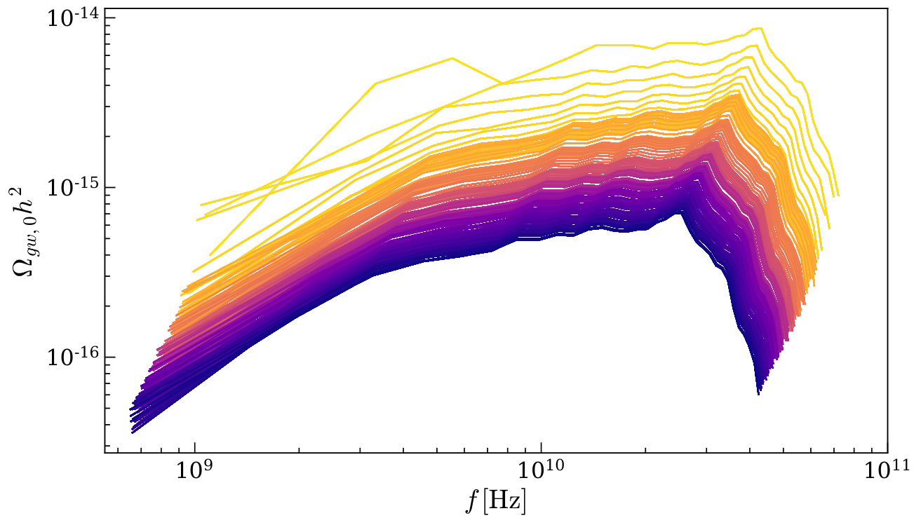
Our lattice simulation results indicate there is no nonlinear self-resonant behavior during preheating and the system does not exhibit any parametric resonant effects when . Results corresponding to are not presented as it requires a higher resolution than is technically achievable in HLattice. Despite the lack of preheating instabilities, instead of solving the coupled ODEs, we use for our numerical simulations the HLattice code which, although more computationally demanding, in principle has a higher precision as it allows us to keep track of the energy conservation (see Eq. (46)).
The lack of an SGWB signal induced by oscillon formation in our simulation results despite the presence of a broad instability band predicted by the Floquet analysis result in Sec. IV requires explanation. The growth of a mode’s amplitude as it passes through an instability band is proportional to the magnitude of and the length of time the mode spends in an instability band. There are several factors that can contribute to the growth’s suppression in our lattice simulations. For instance, the width of the instability band and magnitude of in Fig. 7 both decrease for lower values of . Furthermore, we don’t consider the expansion of the Universe in our Floquet analysis which is expected to suppress the growth of resonant modes. Growth in the SGWB spectrum consistent with oscillon formation is not expected if the amplitude of is not large enough to meaningfully contribute or if the mode doesn’t spend enough time in the instability band. We therefore determine that for the broad self-resonance instability band, the amplitude is not large enough for modes to grow significantly when the expansion of the Universe is considered. In other words, preheating self-resonance is inefficient in the KMII model. It was found in Ref. Turzyński and Wieczorek 2019 that, when the expansion of the Universe is taken into account, the real part of the Floquet exponent does not take any positive value for the KMII potential (with set to ) due to self-resonant effects. This agrees with our lattice simulation results. Note that lowering the value of , which would flatten the curvature of the potential at the minimum, can possibly lead to the formation of oscillon or transient configurations. However, the KMII potential minimum cannot be significantly flattened due to the constraint, which is needed for inflation to end successfully.
We checked that there is no variation in the spectral shape, amplitude, or peak frequency when with and unchanged. We also observe the SGWB spectra are not significantly affected as and are varied within the CI limits of the parameters (see Fig. 5). We find the transfer of energy from the background to the field is negligible when . After the inflaton dynamics settle down, the SGWB spectrum gets “saturated” at . The spectrum thereafter gets gradually redshifted with the expansion of the Universe which results in the amplitude of the SGWB signal that would be observed today to decrease with time. We note that varying the lattice spacing (/) within HLattice can significantly affect the SGWB spectra amplitudes: The amplitude of the SGWB spectrum increases as the lattice simulation resolution is increased. We believe this is because the field fluctuation power spectrum is ultraviolet (UV) divergent and increasing the UV resolution leads to a higher contribution to the SGWB signal. The location of the peak frequency, however, is largely independent of the non-physical simulation parameters. The peak frequency of SGWB signals predicted by preheating in various inflation models typically depends on the characteristic length scale of inflation fragmentation (which can be enhanced due to self-interactions) and the energy scale at which inflation ends (see Ref. Amin et al. 2014 for details). Our SGWB signal result is consistent with this prediction as in the KMII model.
Although good energy conservation cannot be achieved in the simulation runs, a noticeable growth in the SGWB spectra at frequencies is observed when . However, as noted in Ref. Lozanov and Amin 2019, we cannot reliably predict an SGWB signal from preheating that involves inhomogeneities when . Furthermore, the predicted SGWB fluxes in the – range are well outside the range of frequencies that can realistically be probed by any present or near-future GW observatories.
The frequencies of the predicted SGWB fluxes are compared against the Laser Interferometer Gravitational Wave Observatory (LIGO) sensitivity curves Abbott et al. 2019 in Fig. 12. The SGWB spectrum corresponding to was arbitrarily chosen. The figure includes the sensitivity curves from LIGO’s first observing run (O) Abbott et al. 2017, in combination with the second observing run, (O+O) Abbott et al. 2019, and the design sensitivity curve. It is clear from the comparisons in Fig. 12 that the adopted model’s SGWB flux predictions are well beyond the frequency range of the LIGO sensitivity curves. The figure also contains the sensitivity of the proposed graviton–magnon detector Ito and Soda 2020; Ito et al. 2020 and an upper bound at at derived from CMB power spectra, in combination with BAO, lensing, and Deuterium abundance (CMB+BAO+Lensing+2H) observations Pagano et al. 2016. The proposed graviton–magnon detector has sensitivity and at frequencies and , respectively Ito and Soda 2020, which is many orders of magnitude larger than the density of the Universe. The SGWB spectra predictions of the model are below the upper limit set by CMB+BAO+Lensing+2H. The SGWB signal predictions of four other inflation models from the literature are included in Fig. 12 for comparison. The inflation models included are: the E-Model and T-Model inflation (at ) Bhoonah et al. 2021, and Starobinsky and D-brane inflation (resulting from gauge preheating) Adshead et al. 2020. The – frequency range of the SGWB flux predicted by the adopted model is in accord with that of reheating from the other inflation models from the literature used here for comparison. The predicted frequencies of the SGWB fluxes sourced from the adopted model as well as the other inflation models suggest, in order to be probed, future GW observatories need to probe high frequencies in the – range.
VI Conclusions
In an attempt to unify the two phases of accelerated expansions of our Universe within the context of modular inflation, this work studies the viability, effects, and predictions of a simple inflation model known as the Kähler Moduli Inflation I or KMII coupled to a light spectator scalar field . Under the assumption that the total vacuum energy density of the Universe is zero due to some unknown symmetry, the dark energy density , which can be attributed to the observed cosmological constant , is modeled to come from the KMII potential’s non-vanishing minimum. Unfortunately, to achieve this result, the KMII model parameter needs to be almost identical, but not equal, to . This introduces a fine-tuning problem: considering and , the term in the KMII potential must be fine-tuned to decimal places to achieve the desired result.
Our MCMC sampling analysis results estimate the allowed ranges and , both at CI. The predictions can certainly have many implications on cosmology; however, having a large allowed range is not currently practical as it cannot precisely set any constraints. Nonetheless, different cosmological settings, for instance, interactions of the type and couplings to fermions can be incorporated into these analyses in future work to obtain the corresponding lower bounds. This work only considers the standard four-leg interaction term when other types of interactions are at least as well motivated. A detailed study of the effects of the KMII model with different types of interactions would lead to a better understanding of the model’s lower bound predictions on .
Our sampling analysis results indicate the model parameter has the allowed range at CI (see Fig. 5). Implications of this result on being sourced from the KMII potential minimum are in order. Future experiments, particularly, the Next Generation CMB Experiment (CMB-S4) Abazajian et al. 2019 and Simons Observatory Ade et al. 2019 are expected to constrain the CDM parameter values with higher precision. As more precise observational data become available, the MCMC sampling analysis presented here can be applied to determine if the observed data point toward (or equivalently, ). If it does, the energy density due to sourced from the non-vanishing minimum of the KMII potential would remain a possibility. On the other hand, if observations support instead, the additional energy density contribution from the KMII potential would be compounding the cosmological constant problem. The MCMC analysis computes small ranges of the derived CDM parameters , , , and (see Fig. 6) which is attributed to the prior constraints and that were imposed and taking the degeneracies between the CDM parameters into account. It would be possible to determine whether the adopted model is consistent with observations or not using CDM parameter values with higher precision from future observations, particularly, the adopted model would be ruled out if future CMB experiments constrain to be .
The MCMC sampling results (see the off-diagonal plots in Fig. 5) show the correlations between the adopted model parameters , , and can take a wide range of possible values which is primarily due to not having a lower bound. Repeating the MCMC sampling analysis with more precise CDM parameter values, particularly a tighter lower bound on from future observations would allow one to constrain the correlations between the model parameters more precisely, and hence set tighter constraints on and . If future experiments point towards a high , it would have implications on the gravitino mass which is expected to come from the SUSY energy scale. A high can also lead to scenarios where the cosmological gravitino problem is relaxed via, e.g., Planck suppression of the moduli-gravitino coupling, which results in small branching ratios in the gravitino decay modes, avoiding the gravitino overproduction problem. High predictions also have rich implications on particle dark matter models, e.g., it can result in a high abundance of thermal dark matter.
Floquet analysis is performed on the adopted model to compute the Floquet instability charts due to both self- and parametric resonant effects. We observe in our computed results a broad self-resonance band structure at and parametric-resonance bands due to coupling at when the coupling constant . We employ HLattice to numerically simulate the evolution of the fields and compute the mean equation of state parameter , mean field values and , and GW energy spectra. It is demonstrated that always approaches when , and it takes longer for to approach the closer the value of is to zero.
SGWB flux is generated from the adopted model due to field inhomogeneities at frequencies in the – range which is well outside the range of frequencies that can realistically be probed by any present or near-future GW observatories. We do not observe any noticeable growth in the SGWB spectrum from preheating self-resonance instabilities, hence there is no signature of oscillon formations. Although our Floquet analysis predicts a broad self-resonance instability band at , the growth of the resonant field modes is suppressed due to the decreasing width of the instability band and magnitude of for lower values of , and the Hubble friction term which is expected to diminish the magnitude of .
We conclude based on our results that self-resonance is inefficient in the KMII model and the system does not exhibit any parametric resonant effects when . We do not present any numerical results for the adopted model when , as a higher resolution than is technically achievable would be required. In the future, if HLattice can be MPI-parallelized, simulations with a higher resolution may allow one to study in detail the reheating effects of a four-leg interaction term with the KMII model as well as other single-field inflation models that have not been studied with this type of interaction.
We determine the amplitude of SGWB signal sourced from preheating when is dependent on the lattice simulation resolution and cannot be trusted. The SGWB signal amplitude is expected to be roughly static for this range of if the preheating nonlinearities can be captured by running the simulation at a higher resolution. Although the simulations lack good energy conservation, a dramatic increase in the SGWB spectra is observed at frequencies when which is consistent with the Floquet analysis results. The frequencies of these SGWB signals are, however, in the region () where reliable predictions cannot be made.
The predicted frequencies of the SGWB flux are compared against the LIGO sensitivity curves, the sensitivity of the proposed graviton–magnon detector, and SGWB signal predictions of several other inflation models from the literature. The predicted frequencies of the SGWB flux sourced from the model during preheating are all within the known constraints and they are at about the same high-frequency range as that of the other inflation models that are included for comparison. The results point toward the need for future GW observatories to probe high frequencies at the – range to probe SGWB signals sourced from preheating in a number of single-field inflation models. It has been shown that SGWBs can be generated from instabilities in hybrid and multi-field inflation models at frequencies that may be observable by the next generation of GW observatories García-Bellido et al. 2008. Therefore, one possible way to bring the predicted GW frequencies of the adopted model (and other inflation models that can provide a possible source for from the potential’s non-vanishing minimum) to an observable range is incorporating the adopted model with hybrid and multi-field inflation models.
VII Acknowledgements
The authors thank Simran Nerval, Michael Forbes, Sukanta Bose, and Joseph Bramante for valuable discussions and especially Simran Nerval for the helpful pointers on HLattice. This research used resources from the Center for Institutional Research Computing at Washington State University. ACV is supported by the Arthur B. McDonald Canadian Astroparticle Physics Research Institute and NSERC, with equipment funded by the Canada Foundation for Innovation and the Province of Ontario, and housed at the Queen’s Centre for Advanced Computing. Research at Perimeter Institute is supported by the Government of Canada through the Department of Innovation, Science, and Economic Development, and by the Province of Ontario.
References
- Guth (1981) Alan H. Guth, “Inflationary universe: A possible solution to the horizon and flatness problems,” Phys. Rev. D 23, 347–356 (1981).
- Linde (1982a) Andrei D. Linde, “A New Inflationary Universe Scenario: A Possible Solution of the Horizon, Flatness, Homogeneity, Isotropy and Primordial Monopole Problems,” Phys. Lett. B 108, 389–393 (1982a).
- Linde (1982b) Andrei D. Linde, “Coleman-Weinberg Theory and a New Inflationary Universe Scenario,” Phys. Lett. B 114, 431–435 (1982b).
- Albrecht and Steinhardt (1982) Andreas Albrecht and Paul J. Steinhardt, “Cosmology for Grand Unified Theories with Radiatively Induced Symmetry Breaking,” Phys. Rev. Lett. 48, 1220–1223 (1982).
- Linde (1983) Andrei D. Linde, “Chaotic Inflation,” Phys. Lett. B 129, 177–181 (1983).
- de Bernardis et al. (2000) P. de Bernardis, P. A. R. Ade, J. J. Bock, J. R. Bond, J. Borrill, A. Boscaleri, K. Coble, B. P. Crill, G. De Gasperis, P. C. Farese, and et al., “A flat universe from high-resolution maps of the cosmic microwave background radiation,” Nature 404, 955–959 (2000).
- Tegmark et al. (2004) Max Tegmark, Michael A. Strauss, Michael R. Blanton, Kevork Abazajian, Scott Dodelson, Havard Sandvik, Xiaomin Wang, David H. Weinberg, Idit Zehavi, Neta A. Bahcall, and et al., “Cosmological parameters from sdss and wmap,” Physical Review D 69 (2004), 10.1103/physrevd.69.103501.
- Seljak et al. (2005) Uroš Seljak, Alexey Makarov, Patrick McDonald, Scott F. Anderson, Neta A. Bahcall, J. Brinkmann, Scott Burles, Renyue Cen, Mamoru Doi, James E. Gunn, and et al., “Cosmological parameter analysis including sdss ly forest and galaxy bias: Constraints on the primordial spectrum of fluctuations, neutrino mass, and dark energy,” Physical Review D 71 (2005), 10.1103/physrevd.71.103515.
- Blake et al. (2011) Chris Blake, Eyal A. Kazin, Florian Beutler, Tamara M. Davis, David Parkinson, Sarah Brough, Matthew Colless, Carlos Contreras, Warrick Couch, Scott Croom, and et al., “The wigglez dark energy survey: mapping the distance-redshift relation with baryon acoustic oscillations,” Monthly Notices of the Royal Astronomical Society 418, 1707–1724 (2011).
- Dolgov and Linde (1982) A. D. Dolgov and Andrei D. Linde, “Baryon Asymmetry in Inflationary Universe,” Phys. Lett. B 116, 329 (1982).
- Abbott et al. (1982) L. F. Abbott, Edward Farhi, and Mark B. Wise, “Particle Production in the New Inflationary Cosmology,” Phys. Lett. B 117, 29 (1982).
- Kolb and Turner (1990) Edward W. Kolb and Michael S. Turner, The Early Universe, Vol. 69 (Front. Phys., 1990).
- Traschen and Brandenberger (1990) Jennie H. Traschen and Robert H. Brandenberger, “Particle Production During Out-of-equilibrium Phase Transitions,” Phys. Rev. D 42, 2491–2504 (1990).
- Kofman et al. (1994) Lev Kofman, Andrei Linde, and Alexei A. Starobinsky, “Reheating after inflation,” Physical Review Letters 73, 3195–3198 (1994).
- Shtanov et al. (1995) Y. Shtanov, J. Traschen, and R. Brandenberger, “Universe reheating after inflation,” Physical Review D 51, 5438–5455 (1995).
- Cline (2006) James M. Cline, “String Cosmology,” arXiv e-prints , hep-th/0612129 (2006), arXiv:hep-th/0612129 [hep-th] .
- Kallosh (2008) Renata Kallosh, “On inflation in string theory,” Lect. Notes Phys. 738, 119–156 (2008), arXiv:hep-th/0702059 .
- McAllister and Silverstein (2008) Liam McAllister and Eva Silverstein, “String Cosmology: A Review,” Gen. Rel. Grav. 40, 565–605 (2008), arXiv:0710.2951 [hep-th] .
- Kachru et al. (2003a) Shamit Kachru, Renata Kallosh, Andrei D. Linde, and Sandip P. Trivedi, “De Sitter vacua in string theory,” Phys. Rev. D 68, 046005 (2003a), arXiv:hep-th/0301240 .
- Balasubramanian and Berglund (2004) Vijay Balasubramanian and Per Berglund, “Stringy corrections to Kahler potentials, SUSY breaking, and the cosmological constant problem,” JHEP 11, 085 (2004), arXiv:hep-th/0408054 .
- Blanco-Pillado et al. (2004) J. J. Blanco-Pillado, C. P. Burgess, James M. Cline, C. Escoda, M. Gomez-Reino, R. Kallosh, Andrei D. Linde, and F. Quevedo, “Racetrack inflation,” JHEP 11, 063 (2004), arXiv:hep-th/0406230 .
- Balasubramanian et al. (2005) Vijay Balasubramanian, Per Berglund, Joseph P. Conlon, and Fernando Quevedo, “Systematics of moduli stabilisation in Calabi-Yau flux compactifications,” JHEP 03, 007 (2005), arXiv:hep-th/0502058 .
- Conlon and Quevedo (2006a) Joseph P. Conlon and Fernando Quevedo, “Kahler moduli inflation,” JHEP 01, 146 (2006a), arXiv:hep-th/0509012 .
- Blanco-Pillado et al. (2006) J. J. Blanco-Pillado, C. P. Burgess, James M. Cline, C. Escoda, M. Gomez-Reino, R. Kallosh, Andrei D. Linde, and F. Quevedo, “Inflating in a better racetrack,” JHEP 09, 002 (2006), arXiv:hep-th/0603129 .
- Cicoli et al. (2009) M. Cicoli, C. P. Burgess, and F. Quevedo, “Fibre Inflation: Observable Gravity Waves from IIB String Compactifications,” JCAP 03, 013 (2009), arXiv:0808.0691 [hep-th] .
- Dvali and Tye (1999) G. R. Dvali and S. H. Henry Tye, “Brane inflation,” Phys. Lett. B 450, 72–82 (1999), arXiv:hep-ph/9812483 .
- Kachru et al. (2003b) Shamit Kachru, Renata Kallosh, Andrei D. Linde, Juan Martin Maldacena, Liam P. McAllister, and Sandip P. Trivedi, “Towards inflation in string theory,” JCAP 10, 013 (2003b), arXiv:hep-th/0308055 .
- Bond et al. (2007) J. Richard Bond, Lev Kofman, Sergey Prokushkin, and Pascal M. Vaudrevange, “Roulette inflation with Kahler moduli and their axions,” Phys. Rev. D 75, 123511 (2007), arXiv:hep-th/0612197 .
- Binetruy and Dvali (1996) P. Binetruy and G. R. Dvali, “D term inflation,” Phys. Lett. B 388, 241–246 (1996), arXiv:hep-ph/9606342 .
- Gasperini and Veneziano (2016) M. Gasperini and G. Veneziano, “String Theory and Pre-big bang Cosmology,” Nuovo Cim. C 38, 160 (2016), arXiv:hep-th/0703055 .
- Sen (2002) Ashoke Sen, “Rolling tachyon,” JHEP 04, 048 (2002), arXiv:hep-th/0203211 .
- Battefeld and Watson (2006) Thorsten Battefeld and Scott Watson, “String gas cosmology,” Rev. Mod. Phys. 78, 435–454 (2006), arXiv:hep-th/0510022 .
- Khoury et al. (2001) Justin Khoury, Burt A. Ovrut, Paul J. Steinhardt, and Neil Turok, “The Ekpyrotic universe: Colliding branes and the origin of the hot big bang,” Phys. Rev. D 64, 123522 (2001), arXiv:hep-th/0103239 .
- Blanco-Pillado et al. (2010) Jose J. Blanco-Pillado, Duncan Buck, Edmund J. Copeland, Marta Gomez-Reino, and Nelson J. Nunes, “Kahler Moduli Inflation Revisited,” JHEP 01, 081 (2010), arXiv:0906.3711 [hep-th] .
- Davis et al. (2010) Joshua L. Davis, Thomas S. Levi, Mark Van Raamsdonk, and Kevin R. L. Whyte, “Twisted Inflation,” JCAP 09, 032 (2010), arXiv:1004.5385 [hep-th] .
- Barnaby et al. (2009) Neil Barnaby, J. Richard Bond, Zhiqi Huang, and Lev Kofman, “Preheating after modular inflation,” Journal of Cosmology and Astroparticle Physics 2009, 021–021 (2009).
- Antusch et al. (2018) Stefan Antusch, Francesco Cefalà, Sven Krippendorf, Francesco Muia, Stefano Orani, and Fernando Quevedo, “Oscillons from string moduli,” Journal of High Energy Physics 2018 (2018), 10.1007/jhep01(2018)083.
- Kasuya et al. (2020) Shinta Kasuya, Masahiro Kawasaki, Francis Otani, and Eisuke Sonomoto, “Revisiting oscillon formation in the Kachru-Kallosh-Linde-Trivedi scenario,” Phys. Rev. D 102, 043016 (2020), arXiv:2001.02582 [hep-ph] .
- Conlon and Quevedo (2006b) Joseph P Conlon and Fernando Quevedo, “Kähler moduli inflation,” Journal of High Energy Physics 2006, 146–146 (2006b).
- Lee and Nam (2011) Sunggeun Lee and Soonkeon Nam, “Kähler moduli inflation and WMAP7,” Int. J. Mod. Phys. A 26, 1073–1096 (2011), arXiv:1006.2876 [hep-th] .
- Martin et al. (2013) Jerome Martin, Christophe Ringeval, and Vincent Vennin, “Encyclopaedia inflationaris,” (2013), arXiv:1303.3787 [astro-ph.CO] .
- Foreman-Mackey et al. (2013) Daniel Foreman-Mackey, David W. Hogg, Dustin Lang, and Jonathan Goodman, “emcee: The MCMC Hammer,” Publications of the Astronomical Society of the Pacific 125, 306 (2013), arXiv:1202.3665 [astro-ph.IM] .
- Akrami et al. (2020) Y. Akrami, F. Arroja, M. Ashdown, J. Aumont, C. Baccigalupi, M. Ballardini, A. J. Banday, R. B. Barreiro, N. Bartolo, and et al., “Planck 2018 results,” Astronomy & Astrophysics 641, A10 (2020).
- Ade et al. (2018) P. A. R. Ade et al. (BICEP2, Keck Array), “BICEP2 / Keck Array x: Constraints on Primordial Gravitational Waves using Planck, WMAP, and New BICEP2/Keck Observations through the 2015 Season,” Phys. Rev. Lett. 121, 221301 (2018), arXiv:1810.05216 [astro-ph.CO] .
- Martin et al. (2014) Jérôme Martin, Christophe Ringeval, and Vincent Vennin, “Encyclopædia Inflationaris,” Physics of the Dark Universe 5, 75–235 (2014), arXiv:1303.3787 [astro-ph.CO] .
- Giudice et al. (1999) Gian Francesco Giudice, Antonio Riotto, and Igor Tkachev, “Non-thermal production of dangerous relics in the early universe,” Journal of High Energy Physics 1999, 009–009 (1999).
- Kallosh et al. (2000) Renata Kallosh, Lev Kofman, Andrei Linde, and Antoine Van Proeyen, “Gravitino production after inflation,” Phys. Rev. D 61, 103503 (2000).
- Kawasaki et al. (2005) Masahiro Kawasaki, Kazunori Kohri, and Takeo Moroi, “Big-bang nucleosynthesis and hadronic decay of long-lived massive particles,” Physical Review D 71 (2005), 10.1103/physrevd.71.083502.
- Garcia et al. (2020) Marcos A. G. Garcia, Kunio Kaneta, Yann Mambrini, and Keith A. Olive, “Reheating and Post-inflationary Production of Dark Matter,” Phys. Rev. D 101, 123507 (2020), arXiv:2004.08404 [hep-ph] .
- Fornengo et al. (2003) N. Fornengo, A. Riotto, and S. Scopel, “Supersymmetric dark matter and the reheating temperature of the universe,” Physical Review D 67 (2003), 10.1103/physrevd.67.023514.
- Roszkowski et al. (2014) Leszek Roszkowski, Sebastian Trojanowski, and Krzysztof Turzyński, “Neutralino and gravitino dark matter with low reheating temperature,” JHEP 11, 146 (2014), arXiv:1406.0012 [hep-ph] .
- Choi and Takahashi (2017) Ki-Young Choi and Tomo Takahashi, “New bound on low reheating temperature for dark matter in models with early matter domination,” Phys. Rev. D 96, 041301 (2017), arXiv:1705.01200 [astro-ph.CO] .
- Martin and Ringeval (2010) Jérôme Martin and Christophe Ringeval, “First cmb constraints on the inflationary reheating temperature,” Physical Review D 82 (2010), 10.1103/physrevd.82.023511.
- Cook et al. (2015) Jessica L. Cook, Emanuela Dimastrogiovanni, Damien A. Easson, and Lawrence M. Krauss, “Reheating predictions in single field inflation,” JCAP 04, 047 (2015), arXiv:1502.04673 [astro-ph.CO] .
- Drewes et al. (2017) Marco Drewes, Jin U Kang, and Ui Ri Mun, “Cmb constraints on the inflaton couplings and reheating temperature in alpha-attractor inflation,” Journal of High Energy Physics 2017 (2017), 10.1007/jhep11(2017)072.
- Mazumdar and Zaldivar (2014) Anupam Mazumdar and Bryan Zaldivar, “Quantifying the reheating temperature of the universe,” Nucl. Phys. B 886, 312–327 (2014), arXiv:1310.5143 [hep-ph] .
- Trotta (2017) Roberto Trotta, “Bayesian Methods in Cosmology,” (2017) arXiv:1701.01467 [astro-ph.CO] .
- Weinberg (1982) Steven Weinberg, “Cosmological Constraints on the Scale of Supersymmetry Breaking,” Phys. Rev. Lett. 48, 1303 (1982).
- Martin (1998) Stephen P. Martin, “A Supersymmetry primer,” Adv. Ser. Direct. High Energy Phys. 18, 1–98 (1998), arXiv:hep-ph/9709356 .
- Conlon and Quevedo (2007) Joseph P. Conlon and Fernando Quevedo, “Astrophysical and cosmological implications of large volume string compactifications,” JCAP 08, 019 (2007), arXiv:0705.3460 [hep-ph] .
- Bassett et al. (2006) Bruce A. Bassett, Shinji Tsujikawa, and David Wands, “Inflation dynamics and reheating,” Rev. Mod. Phys. 78, 537–589 (2006), arXiv:astro-ph/0507632 .
- Lozanov and Amin (2017) Kaloian D. Lozanov and Mustafa A. Amin, “Equation of State and Duration to Radiation Domination after Inflation,” Phys. Rev. Lett. 119, 061301 (2017), arXiv:1608.01213 [astro-ph.CO] .
- Lozanov and Amin (2018) Kaloian D. Lozanov and Mustafa A. Amin, “Self-resonance after inflation: oscillons, transients and radiation domination,” Phys. Rev. D 97, 023533 (2018), arXiv:1710.06851 [astro-ph.CO] .
- Frolov (2010) Andrei V. Frolov, “Non-linear Dynamics and Primordial Curvature Perturbations from Preheating,” Class. Quant. Grav. 27, 124006 (2010), arXiv:1004.3559 [gr-qc] .
- Karouby et al. (2011) Johanna Karouby, Bret Underwood, and Aaron C. Vincent, “Preheating with the Brakes On: The Effects of a Speed Limit,” Phys. Rev. D 84, 043528 (2011), arXiv:1105.3982 [hep-th] .
- Hertzberg et al. (2014) Mark P. Hertzberg, Johanna Karouby, William G. Spitzer, Juana C. Becerra, and Lanqing Li, “Theory of self-resonance after inflation. I. Adiabatic and isocurvature Goldstone modes,” Phys. Rev. D 90, 123528 (2014), arXiv:1408.1396 [hep-th] .
- Amin et al. (2014) Mustafa A. Amin, Mark P. Hertzberg, David I. Kaiser, and Johanna Karouby, “Nonperturbative Dynamics Of Reheating After Inflation: A Review,” Int. J. Mod. Phys. D 24, 1530003 (2014), arXiv:1410.3808 [hep-ph] .
- Amin (2010) Mustafa A. Amin, “Inflaton fragmentation: Emergence of pseudo-stable inflaton lumps (oscillons) after inflation,” arXiv e-prints (2010), arXiv:1006.3075 [astro-ph.CO] .
- Amin et al. (2012) Mustafa A. Amin, Phillip Zukin, and Edmund Bertschinger, “Scale-dependent growth from a transition in dark energy dynamics,” Phys. Rev. D 85, 103510 (2012).
- Kofman (1996) Lev Kofman, “The Origin of Matter in the Universe: Reheating after Inflation,” arXiv e-prints , astro-ph/9605155 (1996), arXiv:astro-ph/9605155 [astro-ph] .
- Kofman et al. (1997) Lev Kofman, Andrei D. Linde, and Alexei A. Starobinsky, “Towards the theory of reheating after inflation,” Phys. Rev. D 56, 3258–3295 (1997), arXiv:hep-ph/9704452 .
- Greene et al. (1997) Patrick B. Greene, Lev Kofman, Andrei D. Linde, and Alexei A. Starobinsky, “Structure of resonance in preheating after inflation,” Phys. Rev. D 56, 6175–6192 (1997), arXiv:hep-ph/9705347 .
- Huang (2011) Zhiqi Huang, “Art of lattice and gravity waves from preheating,” Phys. Rev. D 83, 123509 (2011), arXiv:1102.0227 [astro-ph.CO] .
- Felder and Tkachev (2008) Gary Felder and Igor Tkachev, “Latticeeasy: A program for lattice simulations of scalar fields in an expanding universe,” Computer Physics Communications 178, 929–932 (2008).
- Sainio (2010) Jani Sainio, “CUDAEASY - a GPU Accelerated Cosmological Lattice Program,” Comput. Phys. Commun. 181, 906–912 (2010), arXiv:0911.5692 [astro-ph.IM] .
- Frolov (2008) Andrei V Frolov, “Defrost: a new code for simulating preheating after inflation,” Journal of Cosmology and Astroparticle Physics 2008, 009 (2008).
- Easther et al. (2010) Richard Easther, Hal Finkel, and Nathaniel Roth, “PSpectRe: A Pseudo-Spectral Code for (P)reheating,” JCAP 10, 025 (2010), arXiv:1005.1921 [astro-ph.CO] .
- Child et al. (2013) Hillary L. Child, John T. Giblin, Jr, Raquel H. Ribeiro, and David Seery, “Preheating with Non-Minimal Kinetic Terms,” Phys. Rev. Lett. 111, 051301 (2013), arXiv:1305.0561 [astro-ph.CO] .
- Sainio (2012) J. Sainio, “PyCOOL - a Cosmological Object-Oriented Lattice code written in Python,” JCAP 04, 038 (2012), arXiv:1201.5029 [astro-ph.IM] .
- Polarski and Starobinsky (1996) David Polarski and Alexei A. Starobinsky, “Semiclassicality and decoherence of cosmological perturbations,” Class. Quant. Grav. 13, 377–392 (1996), arXiv:gr-qc/9504030 .
- Khlebnikov and Tkachev (1996) S. Yu. Khlebnikov and I. I. Tkachev, “Classical decay of inflaton,” Phys. Rev. Lett. 77, 219–222 (1996), arXiv:hep-ph/9603378 .
- Benisty et al. (2020) David Benisty, Eduardo I. Guendelman, Emil Nissimov, and Svetlana Pacheva, “Dynamically generated inflationary cdm,” Symmetry 12, 481 (2020).
- Maggiore (2000) Michele Maggiore, “Gravitational wave experiments and early universe cosmology,” Phys. Rept. 331, 283–367 (2000), arXiv:gr-qc/9909001 .
- Abbott et al. (2018) Benjamin P. Abbott et al. (LIGO Scientific, Virgo), “GW170817: Implications for the Stochastic Gravitational-Wave Background from Compact Binary Coalescences,” Phys. Rev. Lett. 120, 091101 (2018), arXiv:1710.05837 [gr-qc] .
- Vachaspati and Vilenkin (1985) Tanmay Vachaspati and Alexander Vilenkin, “Gravitational Radiation from Cosmic Strings,” Phys. Rev. D 31, 3052 (1985).
- García-Bellido et al. (2008) Juan García-Bellido, Daniel G. Figueroa, and Alfonso Sastre, “Gravitational wave background from reheating after hybrid inflation,” Phys. Rev. D 77, 043517 (2008).
- Turzyński and Wieczorek (2019) Krzysztof Turzyński and Michał Wieczorek, “Floquet analysis of self-resonance in single-field models of inflation,” (2019), arXiv:1808.00835 [astro-ph.CO] .
- Lozanov and Amin (2019) Kaloian D. Lozanov and Mustafa A. Amin, “Gravitational perturbations from oscillons and transients after inflation,” Phys. Rev. D 99, 123504 (2019), arXiv:1902.06736 [astro-ph.CO] .
- Abbott et al. (2019) B. P. Abbott et al. (LIGO Scientific, Virgo), “Search for the isotropic stochastic background using data from Advanced LIGO’s second observing run,” Phys. Rev. D 100, 061101 (2019), arXiv:1903.02886 [gr-qc] .
- Abbott et al. (2017) Benjamin P. Abbott et al. (LIGO Scientific, Virgo), “Upper Limits on the Stochastic Gravitational-Wave Background from Advanced LIGO’s First Observing Run,” Phys. Rev. Lett. 118, 121101 (2017), [Erratum: Phys.Rev.Lett. 119, 029901 (2017)], arXiv:1612.02029 [gr-qc] .
- Ito and Soda (2020) Asuka Ito and Jiro Soda, “A formalism for magnon gravitational wave detectors,” Eur. Phys. J. C 80, 545 (2020), arXiv:2004.04646 [gr-qc] .
- Ito et al. (2020) Asuka Ito, Tomonori Ikeda, Kentaro Miuchi, and Jiro Soda, “Probing GHz gravitational waves with graviton–magnon resonance,” Eur. Phys. J. C 80, 179 (2020), arXiv:1903.04843 [gr-qc] .
- Pagano et al. (2016) Luca Pagano, Laura Salvati, and Alessandro Melchiorri, “New constraints on primordial gravitational waves from Planck 2015,” Phys. Lett. B 760, 823–825 (2016), arXiv:1508.02393 [astro-ph.CO] .
- Bhoonah et al. (2021) Amit Bhoonah, Joseph Bramante, Simran Nerval, and Ningqiang Song, “Gravitational Waves From Dark Sectors, Oscillating Inflatons, and Mass Boosted Dark Matter,” JCAP 04, 043 (2021), arXiv:2008.12306 [hep-ph] .
- Adshead et al. (2020) Peter Adshead, John T. Giblin, Mauro Pieroni, and Zachary J. Weiner, “Constraining Axion Inflation with Gravitational Waves across 29 Decades in Frequency,” Phys. Rev. Lett. 124, 171301 (2020), arXiv:1909.12843 [astro-ph.CO] .
- Abazajian et al. (2019) Kevork Abazajian, Graeme Addison, Peter Adshead, Zeeshan Ahmed, Steven W Allen, David Alonso, Marcelo Alvarez, Adam Anderson, Kam S Arnold, Carlo Baccigalupi, et al., “Cmb-s4 science case, reference design, and project plan,” arXiv preprint arXiv:1907.04473 (2019).
- Ade et al. (2019) Peter Ade, James Aguirre, Zeeshan Ahmed, Simone Aiola, Aamir Ali, David Alonso, Marcelo A. Alvarez, Kam Arnold, Peter Ashton, Jason Austermann, and et al., “The simons observatory: science goals and forecasts,” Journal of Cosmology and Astroparticle Physics 2019, 056–056 (2019).