Jointly Dynamic Topic Model for Recognition of Lead-lag Relationship in Two Text Corpora Journal: Data Mining and Knowledge Discovery

Assume we have two text corpora, i.e., the leading corpus $\mathcal{C}_{lead}$ and the lagged corpus $\mathcal{C}_{lag}$. Both corpora are collected for time $t=1,2,...,T$. Accordingly, the leading corpus and lagged corpus can be split into small datasets according to time. That is, $\mathcal{C}_{lead}=\{\mathcal{C}_{lead,1},...,\mathcal{C}_{lead,T}\}$, and $\mathcal{C}_{lag}=\{\mathcal{C}_{lag,1},...,\mathcal{C}_{lag,T}\}$. In the time slice $t$, assume $\mathcal{C}_{lead,t}$ contains a number of $D_{lead,t}$ documents, while $\mathcal{C}_{lag,t}$ contains a number of $D_{lag,t}$ documents. For each single document $d$ in the two corpora, it contains $N_{d}$ words, which can be represented by $\textbf{w}_{d}=\{w_{d,1},w_{d,2},...,w_{d,N_{d}}\}$.

Given the two text corpora have some content similarities, we assume three types of topics underlying the two corpora. First, assume there are $K$ shared topics, which are represented by both the leading corpus and lagged corpus. Denote the $k$-th shared topic at time $t$ by $\alpha_{t,k}$, which has a probability distribution over the vocabulary of $V$ words. Second, assume there are $J$ lead-specific topics, which are only represented by the leading corpus. Denote the $j$-th lead-specific topic at time $t$ by $\beta_{t,j}$. Last, assume there are $H$ lag-specific topics, which are only represented by the lagged corpus. Denote the $h$-th lag-specific topic at time $t$ by $\gamma_{t,h}$. Both $\beta_{t,j}$ and $\gamma_{t,h}$ have probability distributions over the vocabulary of $V$ words. With the three types of topics, the leading corpus and lagged corpus not only share some similarities, but also have their own content characteristics.

The lead-lag relationship is represented by the shared topics, but with an $l$-period time interval between the leading corpus and lagged corpus. Specifically, for document $d$ in the leading corpus at time $t$, it has a distribution $\theta_{d}$ over $K$ shared topics and $J$ lead-specific topics. Therefore, $\theta_{d}$ is a $(K+J)$-dimensional probability vector. Each word in document $d$ can represent either the shared topics at time $t$ or the lead-specific topics at time $t$. For the document $d^{\prime}$ in the lagged corpus at time $t$, it has a distribution $\phi_{d^{\prime}}$ over $K$ shared topics and $H$ lag-specific topics. Thus $\phi_{d^{\prime}}$ is a $(K+H)$-dimensional probability vector. Given the shared topics in the lagged corpus are $l$-period lagged behind those in the leading corpus, each word in document $d^{\prime}$ can represent the lag-specific topics at time $t$ or the shared topics at time $t+l$. In other words, the shared topics are totally determined by the leading corpus. Once the shared topics are decided by the leading corpus at time $t$, one can forecast the topics underlying the lagged corpus at time $t+l$.

Furthermore, we follow the dynamic topic model (Blei and Lafferty 2006) to characterize the evolution pattern of each topic. Specifically, we model the natural parameters of each topic using a Gaussian process and then map the emitted values to the simplex by softmax transformation. Together with the above assumptions, the generative process of documents is present below:

1. 1.

   For time slice $t=1,2,...,T$:

   1. (a)

      For $1\leq k\leq K$, draw shared topics $\alpha_{t,k}|\alpha_{t-1,k}\sim N(\alpha_{t-1,k},\sigma^{2}_{k}I)$

   2. (b)

      For $1\leq j\leq J$, draw lead-specific topics $\beta_{t,j}|\beta_{t-1,j}\sim N(\beta_{t-1,j},\sigma^{2}_{j}I)$

   3. (c)

      For $1\leq h\leq H$, draw lag-specific topics $\gamma_{t,h}|\gamma_{t-1,h}\sim N(\gamma_{t-1,h},\sigma^{2}_{h}I)$

2. 2.

   For the leading corpus:

   1. (a)

      Draw the mean of topic proportions $\eta_{t}|\eta_{t-1}\sim N(\eta_{t-1},\delta^{2}_{f}I)$

   2. (b)

      For document $d$ whose time stamp is $t_{d}$:

      1. i.

         Draw topic proportions $\theta_{d}\sim N(\eta_{t_{d}},\varpi_{f}^{2}I)$

      2. ii.

         For each word $n$ in this document:

         1. A.

            Draw topic assignment $z_{dn}\sim Multi(\text{softmax}(\theta_{d}))$

         2. B.

            If $z_{dn}$ represents a shared topic, then draw word

            $w_{dn}\sim Multi(\text{softmax}(\alpha_{t_{d},z_{dn}}))$

         3. C.

            If $z_{dn}$ represents a lead-specific topic, then draw word

            $w_{dn}\sim Multi(\text{softmax}(\beta_{t_{d},z_{dn}}))$

3. 3.

   For the lagged corpus:

   1. (a)

      Draw the mean of topic proportions $\kappa_{t}|\kappa_{t-1}\sim N(\kappa_{t-1},\delta^{2}_{l}I)$

   2. (b)

      For document $d^{\prime}$ whose time stamp is $t_{d^{\prime}}$:

      1. i.

         Draw topic proportions $\phi_{d^{\prime}}\sim N(\kappa_{t_{d^{\prime}}},\varpi_{l}^{2}I)$

      2. ii.

         For each word $n$ in this document:

         1. A.

            Draw topic assignment $z_{{d^{\prime}}n}\sim Multi(\text{softmax}(\phi_{d^{\prime}}))$

         2. B.

            If $z_{{d^{\prime}}n}$ represents a shared topic, then draw word

            $w_{{d^{\prime}}n}\sim Multi(\text{softmax}(\alpha_{t_{d^{\prime}}-l,z_{{d^{\prime}}n}}))$

         3. C.

            If $z_{{d^{\prime}}n}$ represents a lag-specific topic, then draw word

            $w_{{d^{\prime}}n}\sim Multi(\text{softmax}(\gamma_{t_{d^{\prime}},z_{{d^{\prime}}n}}))$

In the above generative process, the softmax function maps the mean parameters to the multinomial natural parameters. Denote $x=(x_{1},,,x_{g})^{\top}$ be an arbitrary $g$-dimensional vector. Then $\text{softmax}(x)=\exp(x)/\sum_{i=1}^{g}\exp(x_{i})$. For illustration purpose, the generative process of JDTM is summarized in Figure 2.

We use the method of variational inference for model estimation. Denote the collection of word probabilities for the three types of topics as $\bm{\alpha}=\{\alpha_{t,k}:1\leq t\leq T,1\leq k\leq K\}$, $\bm{\beta}=\{\beta_{t,k}:1\leq t\leq T,1\leq k\leq K\}$, and $\bm{\gamma}=\{\gamma_{t,k}:1\leq t\leq T,1\leq k\leq K\}$. Denote the topic proportions for each document in the two corpora as $\bm{\theta}=\{\theta_{d}:d\in\mathcal{C}_{lead}\}$ and $\bm{\phi}=\{\phi_{d^{\prime}}:d^{\prime}\in\mathcal{C}_{lag}\}$. Denote the collection of topic assignments for all words in the two corpora as $\bm{z}$. Following Blei and Lafferty 2006, we consider $\{\eta_{t}\}$s and $\{\kappa_{t}\}$s as hyperparameters, which are specified in advance. Then the collection of all hyperparameters is $\Lambda=\{\sigma_{k}^{2},\sigma_{j}^{2},\sigma_{h}^{2},\delta_{f}^{2},\delta_{l}^{2},\varpi_{f}^{2},\varpi_{l}^{2},\eta_{t},\kappa_{t}\}$. Given the two text corpora $\mathcal{C}_{lead}$ and $\mathcal{C}_{lag}$, as well as the hyperparameters $\Lambda$, the posterior distribution is derived as follows

By simple calculations, we find the posterior in (1) is intractable. Thus, we employ variational inference (Jordan et al 1999) for model estimation. The idea of variational inference is to posit a distribution family with free parameters (called variational parameters) over the latent variables and then try to find the optimal parameters that can minimize the Kullback-Leibler (KL) divergence to the true posterior.

In our model, we specify the variational distribution to the true posterior in (1) as follows. First, the document-level latent variables follow the same specification as Blei et al 2003. Specifically, for each word $w_{t,d,n}$ from the document $d$ in the leading corpus, its hidden topic assignment $z_{t,d,n}$ is specified by a multinomial distribution with parameter $\lambda_{t,d,n}$. The vector of topic proportions $\theta_{t,d}$ is endowed with a free Dirichlet parameter $\tau_{t,d}$. Recall that the leading corpus only represents the $K$ shared topics and $J$ lead-specific topics. Therefore, $\lambda_{t,d,n}$ and $\tau_{t,d}$ are $(K+J)$-dimensional vectors. Similar specifications are assumed for the lagged corpus, but the variational parameters are all $(K+H)$-dimensional vectors. Second, we assume the specification of topic trajectories following Blei and Lafferty 2006. Specifically, for each type of topics, we posit a dynamic model with Gaussian “variational observations”. For example, for the $k$-th shared topic, we assume its variational distribution is $q(\alpha_{1,k},...,\alpha_{T,k}|\hat{\alpha}_{1,k},...,\hat{\alpha}_{T,k})$. Denote the collection of all variational parameters as $\Gamma$. Given the two corpora are generated independently, the variational distribution is specified as follows

The goal is to solve the optimization problem, i.e, finding the optimal variational parameters that can minimize $KL(q||p)$. This is equivalent to maximizing the evidence lower bound (ELBO),

We optimize the ELBO by using the coordinate ascent method, which iteratively optimizes each parameter in the variational distribution $q$. These updates are repeated until (2) has converged. Below, we discuss the updating formula for each variational parameter.

Topic trajectories. The updates for the topic-level variational parameters do not have a closed form. Following Blei and Lafferty 2006, we adopt a conjugate gradient method based on Kalman filter (Kalman 1960). In general, the updates for the three types of topics are similar. Therefore, we take the update of shared topics as an example. Denote $\hat{\alpha}_{t,k,v}$ as the probability of the $k$-th shared topic on the $v$-th word at time $t$. Then the gradient with respect to $\hat{\alpha}_{t,k,v}$ is,

where $\widetilde{m}_{s,k,v}$ and $\widetilde{V}_{s,k,v}$ are the backward mean and variance, $\hat{\zeta}_{s,k}$ is an additional variational parameter. All the notations are defined as the same as Blei and Lafferty 2006. The only difference among the three types of topics lies in the calculation of $n_{t,k,v}$, which is the number of word $v$ representing the $k$-th topic at time $t$. Specifically, for the shared topic $1\leq k\leq K$, $n_{t,k,v}$ is calculated as follows

where $I(\cdot)$ is the indicator function. For the lead-specific topic $1\leq j\leq J$ and the lag-specific topic $1\leq h\leq H$, the calculation of $n_{t,j,v}$ and $n_{t,h,v}$ are shown below:

Topic proportions and topic assignments. The updates for document-level variational parameters have a closed form as shown in Blei et al 2003. Specifically, the updates for the variational Dirichlet parameters for topic proportions are shown below:

where $d$ and $d^{\prime}$ represent an arbitrary document in the leading corpus and lagged corpus, respectively.

Given the variational topic distributions, we update the variational parameters for topic assignments as follows:

where $\Psi$ is the diagamma function. In each round of recursion, we first update the document-level parameters and then fit the variational observations from expected counts under those document-level variational distributions. Algorithm 1 summarizes the estimation procedure of JDTM.

To handle the problem of large vocabularies, topic models with embeddings have attracted much attentions recently. A notable work is the dynamic embedding topic model (Dieng et al 2019), which represents dynamic topics in embedding spaces. Specifically, for each topic $k$ at a given time $t=1,...,T$, its word probabilities $\beta_{t,k}$ is represented by an $L$-dimensional vector, i.e., $\beta_{t,k}\in\mathcal{R}^{L}$. Each word in the vocabulary is also represented by an embedding vector. Suppose the vocabulary has $V$ distinct words, then the word embedding matrix $\rho$ is a $L\times V$ matrix. The probability of each word under each topic is given by the exponentiated inner product between the embedding representations of the word and the topic at the corresponding time, i.e., $p(w_{d,n}=v|z_{d,n}=k,\beta_{t_{d},k})\propto\exp\{\rho_{v}^{\top}\beta_{t_{d},k}\}$. Then similarly with DTM, the evolution of topic probabilities is modeled by a Gaussian distribution with variance $\sigma^{2}$, i.e., $\beta_{t,k}|\beta_{t-1,k}\sim N(\beta_{t-1,k},\sigma^{2}I)$.

Following the idea of (Dieng et al 2019), we propose the jointly dynamic embedding topic model (JDETM), which extends JDTM with the embedding techniques. In general, all the notations are the same as JDTM, except for the topic probabilities, which are represented by embeddings. That is, we assume $\alpha_{t,k},\beta_{t,j},\gamma_{t,h}\in\mathcal{R}^{L}$ for the three types of topics. In JDETM, we marginalize out the topic assignments $\bm{z}$ and regard the Gaussian priors $\eta_{t}$ and $\kappa_{t}$ as latent variables. Denote $\bm{\eta}=\{\eta_{t}:1\leq t\leq T\}$ and $\bm{\kappa}=\{\kappa_{t}:1\leq t\leq T\}$. Then all latent variables to be estimated in JDETM are $(\bm{\alpha},\bm{\beta},\bm{\gamma},\bm{\theta},\bm{\phi},\bm{\eta},\bm{\kappa})$. Denote $\widetilde{\Lambda}$ be the collection of all hyperparameters. Then the posterior distribution in JDETM is $\widetilde{p}=p(\bm{\alpha},\bm{\beta},\bm{\gamma},\bm{\theta},\bm{\phi},\bm{\eta},\bm{\kappa}|\mathcal{C}_{lead},\mathcal{C}_{lag},\widetilde{\Lambda})$.

We still use variational inference for model estimation. Following the inference procedure of DETM Dieng et al 2019, we preserve some of the conditional dependencies of the graphical model through the structured variational family (Saul and Jordan 1995). We assume the parameters of the approximated distributions as the functions of the data (Kingma and Welling 2013). Specifically, for any document $d$ in the leading corpus with its timestamp $t_{d}$, we model the variational mean and variance of topic proportions as a function of the latent prior $\eta_{t_{d}}$ and all words in this document $\textbf{w}_{d}$. The latent prior $\eta_{t_{d}}$ is represented by all the previous latent priors $\eta_{1:{t_{d}}-1}$ and the normalized representations of words in all leading documents $\mathcal{C}_{lead,t}$. The specifications of the variational parameters for the lagged corpus are the same as those for the leading corpus. Denote all the variational parameters as $\widetilde{\Gamma}$. Then, the variational distribution in JDETM has the following form

Under these assumptions, we model the topic proportions by feed-forward neural networks and the latent priors by LSTM Hochreiter and Schmidhuber 1997. Our goal is to maximize the ELBO (i.e., $\text{E}_{q}\left[\log\widetilde{p}-\log\widetilde{q}\right]$) with respective to the variational parameters $\widetilde{\Gamma}$. With the reparameterization trick in Kingma and Welling 2013, we can obtain gradients by using the back propagation method and then optimize the variational parameters. In particular, we use the method of stochastic gradient descent and set the learning rate by Adam Kingma and Ba 2015. Algorithm 2 summarizes the estimation procedure of JDETM.

To demonstrate the performance of our proposed jointly dynamic topic modeling approach, we design a variety of experiments on synthetic data. Given topics models are all probabilistic generative models, we can generate synthetic documents according to the generative process illustrated in Figure 2. Under a fixed time span $T$ and the numbers of three types of topics (i.e., $K$, $J$ and $H$), we first present the generation process for topic proportions, i.e., $\{\theta_{d}\}$s of the leading corpus and $\{\phi_{d^{\prime}}\}$s of the lagged corpus. First, we randomly generate the initial values of the topic proportion means $\eta_{0}$ and $\kappa_{0}$ from the standard normal distribution $N(0,1)$. Second, for time $1\leq t\leq T$, the topic proportion means $\eta_{t}$ and $\kappa_{t}$ are generated from normal distributions $N(\eta_{t-1},1)$ and $N(\kappa_{t-1},1)$, respectively. Last, given all topic proportion means, the topic proportions $\{\theta_{d}\}$s and $\{\phi_{d^{\prime}}\}$s are generated from log-normal distributions $LN(\eta_{t_{d}},1)$ and $LN(\kappa_{t_{d^{\prime}}},1)$, respectively. Next, we generate documents under two scenarios to investigate the performance of JDTM and JDETM.

Scenario 1. In this scenario, we generate documents under the generation procedure of JDTM. Specifically, we set the time span $T=10$ and the vocabulary size $V=1000$. For $K$ shared topics, $J$ lead-specific topics and $H$ lag-specific topics, the topic probabilities are initially generated from the standard normal distribution $N(0,1)$ and then evolve with Gaussian noises, e.g., $\alpha_{t,k}\sim N(\alpha_{t-1,k},1)$. For time $1\leq t\leq T$, the number of documents $D_{lead,t}$ and $D_{lag,t}$ are both generated from the Poisson distribution $Po(100)+50$. For each document in the leading corpus or the lagged corpus, the number of words is generated from the Poisson distribution $Po(50)+50$.

Scenario 2. In this scenario, we generate large document corpus under the generation procedure of JDETM. To obtain the topic embeddings and word embeddings, we follow (Dieng et al 2019) to apply DETM on the ACL dataset with a total of 50 topics. Then, we split the 50 topics into $J$ lead-specific topics, $H$ lag-specific topics, and $K$ shared topics. The JS-divergence is calculated between distributions of lead-specific topics and lag-specific topics to guarantee certain differences between the two types of topics. Then, following the ACL dataset, we set the time span $T=31$ and the vocabulary size $V=17,794$. For time $1\leq t\leq T$, the number of documents $D_{lead,t}$ and $D_{lag,t}$ are both generated from the Poisson distribution $Po(400)+100$. For each document in the leading corpus or the lagged corpus, the number of words is generated from the Poisson distribution $Po(300)+50$.

In the proposed model, the lead-lag relationship is characterized by the shared topics. Therefore, the proportion of shared topics (i.e., $K$) among all topics (i.e., $K+J+H$) can represent the strength of lead-lag relationship. To consider different strengths of lead-lag relationship, we change the numbers of three types of topics to mimic the situation of no lead-lag relationship, weak lead-lag relationship and strong lead-lag relationship. In each situation, we consider the lagged time period $l=1,3,5$. As a result, we have a combination of 2 scenarios $\times$ 3 situations $\times$ 3 lagged values $=18$ experimental settings. In each setting, we repeat the experiment for 20 times.

We compare our model with two approaches. In the first approach, we apply the DTM or the DETM to fit the leading corpus and lagged corpus, separately. We denote this separately modeling approach as $\text{DTM}_{\text{s}}$ and $\text{DETM}_{\text{s}}$. In this approach, the numbers of topics set for the leading corpus and the lagged corpus are $K+J$ and $K+H$, respectively. In the second approach, we combine the leading corpus and the lagged corpus together and then apply the DTM or DETM. We denote this modeling approach as $\text{DTM}_{\text{c}}$ and $\text{DETM}_{\text{c}}$. In this approach, the number of topics set for the combined corpora is $K+J+H$.

We use the document completion perplexity (Wallach et al 2009) to evaluate the model performance. The task of document completion aims to estimate the probability of the second half of a document given its first half. Let $d^{(1)}$ be the first half of document $d$ and $d^{(2)}$ be the second half. Then the completion perplexity of corpus $\mathcal{C}$ is computed as follows,

where $\mathcal{M}$ is the fitted model and $p(d^{(2)}|d^{(1)},\mathcal{M})=\prod^{N_{d}}_{i=1}p(z_{i}|d^{(1)},\mathcal{M})p(w_{i}|z_{i})$. The lower the perplexity, the better the model performance.

Table 1 shows the averaged document completion perplexities among 20 experiments in each experimental setting in scenario 1. For each method, we compare the perplexity on the leading corpus, the lagged corpus, as well as the combination of two corpora. For easy understanding, we also calculate the lift proportions between the perplexities in JDTM and its competitors. As shown by Table 1, under the situation of no lead-lag relationship, the JDTM obtains comparable results with DTMs. In addition, both the two methods have largely outperformed DTMc. However, when there exists weak lead-lag relationship or strong lead-lag relationship, the JDTM can outperform DTMs and DTMc. Particularly, the JDTM has shown greater advantages in the lagged corpus than in the leading corpus. In addition, with the stronger lead-lag relationship, the advantages of JDTM on the lagged corpus becomes more obvious.

Table 2 shows the averaged document completion perplexities in scenario 2. In general, the results in Table 2 show similar trends with those in Table 1. When there is no lead-lag relationship, JDETM and DETMs have outperformed DETMc. When there exists weak lead-lag relationship or strong lead-lag relationship, the JDETM shows advantages over the other methods. Specifically, regarding the estimation performance in the leading corpus, the JDETM can achieve the best or comparable performance with its competitors. In terms of the estimation performance in the lagged corpus or the combination of the two corpora, the JDETM can always outperform all the other models, and its advantages are more obvious.

In this section, we try to apply the jointly dynamic topic model to investigate the influences of academic papers on students’ scientific researches. To this end, we take the field of statistics as an example, and collect two text corpora as follows. The first text corpus is statistical papers published on top journals. Specifically, according to the number of journal citations in Web of Science (i.e., the Journal Citation Report in 2019), ten journals with the highest number of citations are selected under the category of Statistics and Probability. Then, all papers published on these ten journals from 2005 to 2019 are crawled. It results in a total of 12,348 papers. For each paper, its authors, published time, abstract and keywords are collected. The abstracts are then used as the leading corpus, which is denoted as EN. The second text corpus is the Chinese graduation theses majored in statistics. Specifically, we focus on the Chinese master graduation theses majored in Statistics or Probability Theory and Mathematical Statistics. We crawl these theses published between 2005 to 2019 from the CNKI Database.¹¹ 1 https://epub.cnki.net/kns/brief/result.aspx?dbPrefix=CDMD It results in a total of 12,903 theses. For each thesis, its author, published time, graduation school, abstract and keywords are collected. The abstracts in all graduation theses are considered as the lagged corpus, which is denoted as CN. The ten selected journals for the leading corpus are listed in Appendix A. For illustration purpose, Appendix A also presents the names of ten universities with the largest number of theses in the lagged corpus.

For each corpus, we first preprocess the text documents by removing stop words. Given the lagged corpus is written in Chinese, word segmentation using an open-source package Jieba is performed. Then, we remove words with document frequencies higher than 70% or appearing in less than 10 documents from both corpora. Finally, to match the written language in the leading corpus and lagged corpus, we apply the Baidu Translator²² 2 https://fanyi.baidu.com/ to translate Chinese words into English. After all these preprocessing steps, the total vocabulary size is $V=8,611$.

We organize the two corpora in the yearly format, which results in 15 years in total. The numbers of documents in the two corpora in each year are shown in Figure 3. As shown, the number of published papers is relatively stable across year, which is mainly due to the journals’ issue policies. On the other hand, there is an obvious increasing trend in the number of graduation theses. This indicates the enrollment of gradate students is expanding in China.

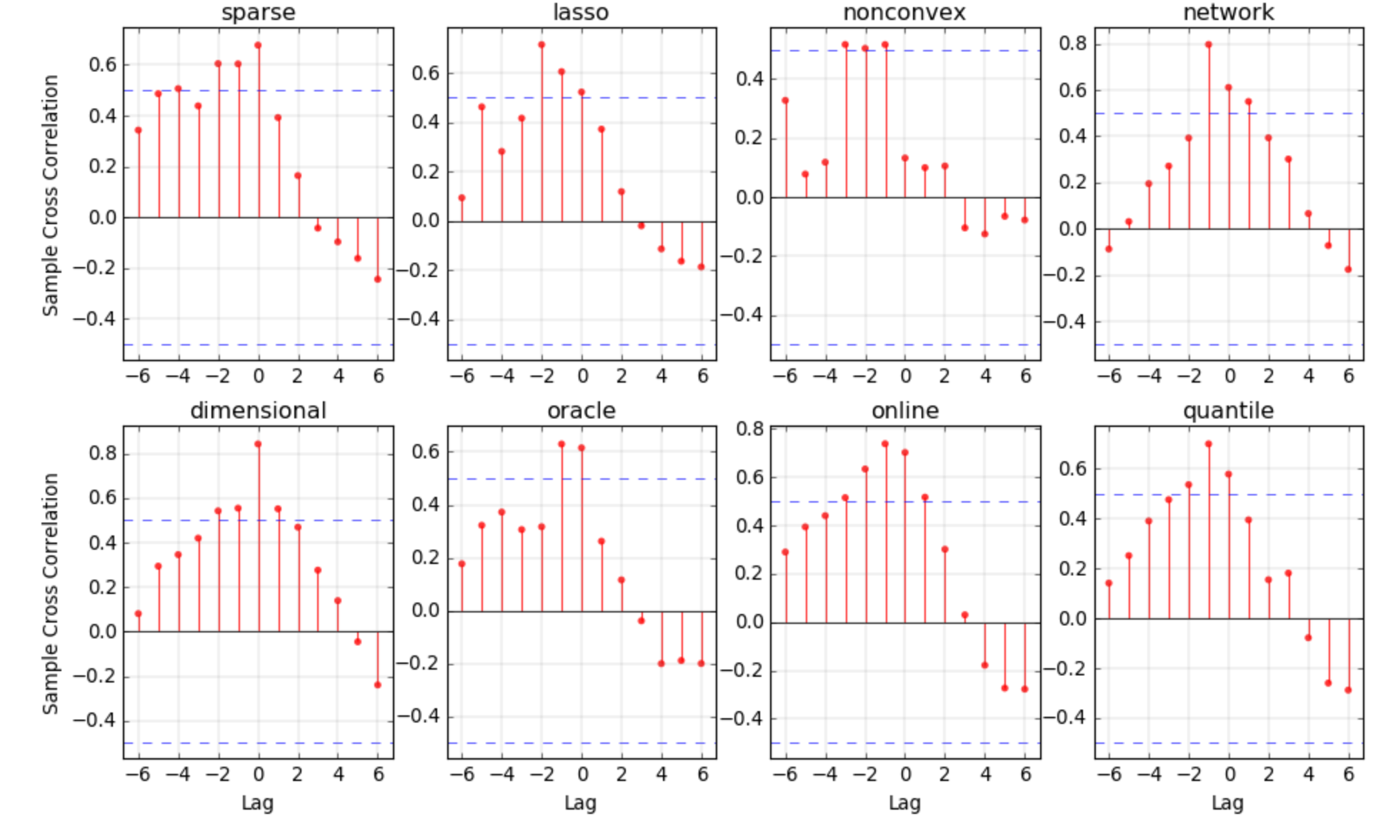
We then explore the potential lead-lag relationship in the two corpora by applying some time series tools. We first choose eight example words, which represent classic topics in statistics. They are, “sparse”, “lasso”, “nonconvex”, “network”, “dimensional”, “oracle”, “online”, and “quantile”, respectively. For each word $w$, we calculate its yearly frequencies in the two corpora, and regard them as two time series which are denoted by $\text{EN}_{w}$ and $\text{CN}_{w}$. We then draw the lagged cross correlation plot (Cryer and Chan 2008) for the two time series. The corresponding results are shown in Figure 4. It is obvious that, all the eight words have significant lagged correlation coefficients around lag -2 to 2, as their coefficient bars exceed the corresponding confidence intervals. These results suggest that, the time series of the EN corpus predates uptrend that of the CN corpus. These results motivate us to further explore the lead-lag relationship between the two corpora by the jointly dynamic topic model.

We then apply the jointly dynamic topic modeling approach to explore the relationship between the statistical papers and graduation theses. Given the two text corpora are of large scale, we choose the JDETM for analysis. For illustration purpose, we set $K=10$ shared topics, $J=10$ lead-specific topics, and $H=10$ lag-specific topics. Following Dieng et al 2019, we set the hyperparameters as $\sigma^{2}_{k}=\sigma^{2}_{j}=\sigma^{2}_{h}=0.005$ and $\varpi_{f}^{2}=\varpi_{l}^{2}=1$. To evaluate the performance of JDETM, we also take $\text{JDETM}_{\text{s}}$ and $\text{JDETM}_{\text{c}}$ as competitors. The number of topics set in $\text{JDETM}_{\text{s}}$ and $\text{JDETM}_{\text{c}}$ are 20 and 30, respectively. To explore the lead-lag relationship in the two corpora, we consider the lagged time period as $l=1,2,3$.

We split the leading corpus and lagged corpus into three parts, i.e., the training dataset (85%), the validation dataset (5%) and the test dataset (10%). The training dataset and validation dataset are used for model estimation, while the test dataset is used for model evaluation. For all embedding topic models, we use randomly initialized 300-dimensional word embeddings. We then employ stochastic variational inference with a batch size of 200 documents and take a training procedure for 400 epochs. For the topic proportions $\{\theta_{d}\}$s and $\{\phi_{d^{\prime}}\}$s, we use a fully connected feed-forward network with 2 layers of 800 hidden units and ReLU activations. Given the length of documents is not long, we fix the means of latent proportions as $\eta=\kappa=0.1$, which can reduce the model complexity and prevent overfitting. The learning rates in all methods are fixed as 0.001.

Table 3 shows the performance of JDETM and its competitors on the test dataset. We can draw the following conclusions. First, the method of $\text{DETM}_{\text{c}}$ achieves the worse performance in both the leading corpus and lagged corpus. This finding suggests that simply combining the two types of documents would not improve the performance of topic learning, even though more information is considered. Second, the JDETM has achieved the best performance in the lagged corpus, while kept comparable performance with $\text{DETM}_{\text{s}}$ in the leading corpus. These results verify the superiority of JDETM in modeling the lagged corpus. It is also notable that, compared with $\text{DETM}_{\text{s}}$, JDETM only needs to be trained once, which is more convenient for practical applications.

In this subsection, we try to investigate the specific patterns and shared patterns in the two corpora. As we mentioned before, the shared topics capture the similarities of the two corpora, while the lead-specific topics and lag-specific topics capture the characteristics in each single corpus. Therefore, by analyzing the top words with highest probabilities in the three types of topics, we can have a general idea about the specific and shared patterns of the two corpora. To illustrate this idea, we randomly choose two lead-specific topics (“Fuzzy System” and “High-dimensional Statistics”), two lag-specific topics (“Inequality Problems in China” and “Evaluation Index”), and four shared topics (“Economic Development”, “Parameter Estimation”, “Financial Markets”, and “Model Selection”) under the JDETM with $l=1$ as examples. We name the topics by summarizing the meanings of words with high probabilities under each topic. Then, we select the top six words with the highest probabilities in each example topic, and show their probability trends across time in Figure

As shown, the top words in the chosen topics are in agreement with the characterisers of the two corpora. For example, documents related to fuzzy system mainly appear in the journal Fuzzy Sets and Systems. Therefore, the topic “Fuzzy System” has been recognized as a lead-specific topic. In addition, the topics “Inequality Problems in China” and “Evolution Index” are mainly discussed by Chinese students in their graduation theses, and thus these two topics appear as lag-specific topics. Regarding the four shared topics, they are common themes discussed in the field of statistics, such as the parameter estimation and financial markets. As a consequence, these shared topics recognized by JDETM reflect the common interests of the two corpora.

Next, we take the eight topics shown in Figure 5 as examples to further demonstrate the lead-lag relationship recognized by JDETM. Note that we have found the top six words with the highest probabilities for each topic, which represent the main meanings of the topics. We then test whether the causal relationship exists for each word in the two corpora. Specifically, for each word $w$, we regard its yearly frequencies $\text{EN}_{w}$ and $\text{CN}_{w}$ as two time series. Then we test the causality of the two time series via the convergent cross mapping (CCM) method Sugihara et al 2012. The main idea of the CCM method is that, if the time series $\text{EN}_{w}$ causally influences the time series $\text{CN}_{w}$, the historical records of $\text{EN}_{w}$ can be reliably predicted through the manifold generated from $\text{CN}_{w}$. Thus we can test for causation through the correlation between the true values and predicted values of $\text{EN}_{w}$. We apply the CCM method for each word in the eight topics, and the detailed results are shown in Table 4. As shown, most top words under the four shared topics (14 out of 24) have significantly causal relationships between the two corpora. On the contrary, most top words under the lead-specific topics and lag-specific topics are insignificant (only 4 out of 24 are significant) or even unpredictable (denoted by “-”). These results imply the existence of the underlying causality in the two corpora, which are consistent with the lead-lag relationship discovered by JDETM.

We focus on the recognized lead-lag relationship between the two corpora in this subsection. First, we try to verify the idea that, the existence of lead-lag relationship can improve the performance of topic modeling in the lagged corpus. Recall that we have applied the JDETM and $\text{DETM}_{\text{s}}$ on the academic corpora, and calculated the perplexity for each test document under the two models. Then, we compute the perplexity difference between the two methods for each test document in the lagged corpus. Next, we select test documents, whose perplexity differences are among the top 10% or bottom 10% in the lagged corpus. In other words, the JDETM has performed much better than $\text{DETM}_{\text{s}}$ on the top 10% documents; while achieved much worse performance than $\text{DETM}_{\text{s}}$ on the bottom 10% documents. We take JDETM with the lagged time period equal to 1 and 2 for illustration. Figure 6 presents the averaged topic proportions of these selected documents. Note that all these selected documents are in the lagged corpus, therefore they only have topic proportions on the lag-specific topics as well as the shared topics. As shown, the top 10% documents usually have higher probabilities on the shared topics; while the bottom 10% documents have relatively lower probabilities on the shared topics. Therefore, the shared topics contribute to the topic representations of documents (as measured by perplexity) in JDETM. Further recall the lead-lag relationship between the leading corpus and lagged corpus is characterized by the shared topics. These results demonstrate that, by recognizing the lead-lag relationship embedded in the shared topics, the JDETM can improve the quality of topic representations in the lagged corpus.

Next, we examine the lead-lag relationship discovered by our model. For illustration purpose, we randomly select two shared topics estimated by the JDETM with the lag time period $l=1$. Then in each time period, we select documents having the largest proportions in this topic from both corpora. Next, we find the most commonly used words in these documents. Figure 7 shows the evolution of eight most commonly used words in the selected documents in the leading corpus and lagged corpus. As shown, the commonly used words in the leading corpus at time $t$ are very similar with those used in the lagged corpus at time $t+1$. Furthermore, the evolution of words in the shared topic “Model Selection” shows the temporal changes in academic hotspots: from the linear regression models in early years, to various variable selection methods (e.g., Lasso), and more recently nonparametric methods and general discussions about regularization and penalty. These results imply the content influences of the leading corpus made on the lagged corpus. It further verifies the existence of the lead-lag relationship between the two corpora.

Finally, we discuss the forecast ability of our proposed method. The lead-lag relationship can help predict the topics to be discussed by the lagged corpus in the future. Specifically, the lead-lag relationship in JDETM is represented by the shared topics with an $l$-period time interval between the leading corpus and lagged corpus. As a consequence, the shared topics discussed by the leading corpus at the last time slice $T$ should also be discussed by the lagged corpus at the future time slice $T+l$. By this way, the JDETM can predict the future topics to be discussed by the lagged corpus. In Table 5, we provide the ten shared topics discussed by the English journal papers in the last year 2019. For each topic, the top seven words with the highest probabilities are reported. As suggested by JDETM, these topics would be talked about by the Chinese thesis in the year 2020.

References

- Ahmed and Xing (2008) Ahmed A, Xing EP (2008) Dynamic non-parametric mixture models and the recurrent Chinese restaurant process: with applications to evolutionary clustering. In: Proceedings of the SIAM International Conference on Data Mining, SDM 2008, April 24-26, 2008, Atlanta, Georgia, USA, pp 219–230
- Ahmed and Xing (2010) Ahmed A, Xing EP (2010) Timeline: A dynamic hierarchical Dirichlet process model for recovering birth/death and evolution of topics in text stream. In: Proceedings of the Twenty-Sixth Conference on Uncertainty in Artificial Intelligence, Catalina Island, CA, USA, July 8-11, 2010, pp 20–29
- AlSumait et al (2008) AlSumait L, Barbara D, Domeniconi C (2008) On-line LDA: adaptive topic models for mining text streams with applications to topic detection and tracking. In: Proceedings of the 8th IEEE International Conference on Data Mining, pp 3–12
- Ashley et al (1980) Ashley R, Granger CWJ, Schmalensee R (1980) Advertising and aggregate consumption: An analysis of causality. Econometrica 48(5):1149–1167
- Blei and Lafferty (2006) Blei DM, Lafferty JD (2006) Dynamic topic models. In: Proceedings of the Twenty-Third International Conference (ICML 2006), Pittsburgh, Pennsylvania, USA, June 25-29, 2006, pp 113–120
- Blei et al (2003) Blei DM, Ng AY, Jordan MI (2003) Latent Dirichlet allocation. The Journal of Machine Learning Research 3:993–1022
- Chae et al (2012) Chae J, Thom D, Bosch H, Yun J, Maciejewski R, Ebert DS, Ertl T (2012) Spatiotemporal social media analytics for abnormal event detection and examination using seasonal-trend decomposition. In: IEEE Conference on Visual Analytics Science & Technology, pp 143–152
- Chen et al (2019) Chen J, Gong Z, Liu W (2019) A nonparametric model for online topic discovery with word embeddings. Information Sciences 504:32–47
- Costa and Ortale (2021) Costa G, Ortale R (2021) Jointly modeling and simultaneously discovering topics and clusters in text corpora using word vectors. Information Sciences 563:226–240
- Cryer and Chan (2008) Cryer JD, Chan KS (2008) Time Series Analysis: With Applications in R. Springer
- Dieng et al (2019) Dieng AB, Ruiz FJR, Blei DM (2019) The dynamic embedded topic model. arXiv preprint arXiv:190705545
- Dieng et al (2020) Dieng AB, Ruiz FJR, Blei DM (2020) Topic modeling in embedding spaces. Transactions of the Association for Computational Linguistics 8:439–453
- Dubey et al (2013) Dubey A, Hefny A, Williamson S, Xing EP (2013) A nonparametric mixture model for topic modeling over time. In: Proceedings of the SIAM International Conference on Data Mining, pp 530–538
- Granger (1969) Granger CWJ (1969) Investigating causal relations by econometric models and cross-spectral methods. Econometrica 37(3):424–438
- He et al (2015) He J, Chen X, Du M, Jiang H (2015) Topic evolution analysis based on improved online LDA model. Journal of Central South University (Science and Technology) 46(2):547–553
- Hochreiter and Schmidhuber (1997) Hochreiter S, Schmidhuber J (1997) Long short-term memory. Neural Computation 9(8):1735–1780
- Jordan et al (1999) Jordan MI, Ghahramani Z, Jaakkola TS, Saul LK (1999) An introduction to variational methods for graphical models. Machine Learning 37(2):183–233
- Kalman (1960) Kalman RE (1960) A new approach to linear filtering and prediction problems. Journal of Basic Engineering 82(1):35–45
- Kawamae (2011) Kawamae N (2011) Trend analysis model: trend consists of temporal words, topics, and timestamps. In: Proceedings of the fourth ACM international conference on Web search and data mining, pp 317–326
- Kingma and Ba (2015) Kingma DP, Ba JL (2015) Adam: A method for stochastic optimization. In: International Conference on Learning Representations 2015, pp 1–15
- Kingma and Welling (2013) Kingma DP, Welling M (2013) Auto-encoding variational Bayes. In: International Conference on Learning Representations(ICLR), pp 1–14
- Meng et al (2017) Meng H, Xu HC, Zhou WX, Sornette D (2017) Symmetric thermal optimal path and time-dependent lead-lag relationship: novel statistical tests and application to uk and us real-estate and monetary policies. Quantitative Finance 17(6):959–977
- Mohamad and Bouchachia (2019) Mohamad S, Bouchachia A (2019) Online Gaussian LDA for unsupervised pattern mining from utility usage data. arXiv:191011599
- Nallapati et al (2007) Nallapati RM, Ditmore S, Lafferty JD, Ung K (2007) Multiscale topic tomography. In: ACM Sigkdd International Conference on Knowledge Discovery & Data Mining, pp 520–529
- Pozdnoukhov and Kaiser (2011) Pozdnoukhov A, Kaiser C (2011) Space-time dynamics of topics in streaming text. In: ACM Sigspatial International Workshop on Location-based Social Networks, pp 1–8
- Rudolph and Blei (2018) Rudolph M, Blei D (2018) Dynamic embeddings for language evolution. In: Proceedings of the 2018 World Wide Web Conference, pp 1003–1011
- Runge et al (2019) Runge J, Bathiany S, Bollt E, Camps-Valls G, Zscheischler J (2019) Inferring causation from time series in earth system sciences. Nature Communications 10(1):2553–2553
- Sasaki et al (2014) Sasaki K, Yoshikawa T, Furuhashi T (2014) Online topic model for Twitter considering dynamics of user interests and topic trends. In: Proceedings of the Conference on Empirical Methods in Natural Language Processing, pp 1977–1985
- Saul and Jordan (1995) Saul LK, Jordan MI (1995) Exploiting tractable substructures in intractable networks. Advances in Neural Information Processing Systems 8:486–492
- Sornette and Zhou (2005) Sornette D, Zhou W (2005) Non-parametric determination of real-time lag structure between two time series: the “optimal thermal causal path” method. Quantitative Finance 5(6):577–591
- Sugihara et al (2012) Sugihara G, May RM, Ye H, hao Hsieh C, Deyle ER, Fogarty MJ, Munch SB (2012) Detecting causality in complex ecosystems. Science 338(6106):496–500
- Vavliakis et al (2012) Vavliakis KN, Tzima FA, Mitkas PA (2012) Event detection via LDA for the mediaeval 2012 sed task. In: MediaEval Workshop, pp 1–2
- Wallach et al (2009) Wallach HM, Murray I, Salakhutdinov R, Mimno D (2009) Evaluation methods for topic models. In: Proceedings of the 26th Annual International Conference on Machine Learning, pp 1–8
- Wang et al (2008) Wang C, Blei D, Heckerman D (2008) Continuous time dynamic topic models. Uncertainty in Artificial Intelligence pp 579–586
- Wang and Mccallum (2006) Wang X, Mccallum A (2006) Topics over time: A non-markov continuous-time model of topical trends. In: Proceedings of the ACM SIGKDD International Conference on Knowledge Discovery and Data Mining, pp 424–433
- Yang et al (2019) Yang M, Qu Q, Chen X, Tu W, Shen Y, Zhu J (2019) Discovering author interest evolution in order-sensitive and semantic-aware topic modeling. Information Sciences 486:271–286
- Ye et al (2015) Ye H, Deyle ER, Gilarranz LJ, Sugihara G (2015) Distinguishing time-delayed causal interactions using convergent cross mapping. Scientific Reports 5(1):14,750–14,750
- Zhou et al (2017) Zhou H, Huimin YU, Roland HU (2017) Topic evolution based on the probabilistic topic model: a review. Frontiers of Computer Science 11(5):786–802
- Zhou and Chen (2014) Zhou X, Chen L (2014) Event detection over Twitter social media streams. The VLDB Journal 23(3):381–400