Exact Convergence Analysis for Metropolis-Hastings Independence Samplers in Wasserstein Distances
Abstract
Under mild assumptions, we show the exact convergence rate in total variation is also exact in weaker Wasserstein distances for the Metropolis-Hastings independence sampler. We develop a new upper and lower bound on the worst-case Wasserstein distance when initialized from points. For an arbitrary point initialization, we show the convergence rate is the same and matches the convergence rate in total variation. We derive exact convergence expressions for more general Wasserstein distances when initialization is at a specific point.
Using optimization, we construct a novel centered independent proposal to develop exact convergence rates in Bayesian quantile regression and many generalized linear model settings. We show the exact convergence rate can be upper bounded in Bayesian binary response regression (e.g. logistic and probit) when the sample size and dimension grow together.
1 Introduction
Applications in modern statistics often require generating Monte Carlo samples from a distribution defined on using a version of the Metropolis-Hastings algorithm [4, 15, 29]. Popular versions of Metropolis-Hastings include, among many others, random walk Metropolis-Hastings, Metropolis-adjusted Langevin algorithm, Metropolis-Hastings independence (MHI) sampler, and Hamiltonian Monte Carlo.
Convergence analyses of general state space Metropolis-Hastings algorithms have traditionally focused on studying their convergence rates in total variation distances [30, 43, 47]. These convergence rates have received significant attention, at least in part, because they provide a key sufficient condition for the existence of central limit theorems [21] and the validity of methods for assessing the reliability of the simulation effort [42, 48]. However, convergence analyses of Metropolis-Hastings Markov chains typically result in qualitative convergence rates [14, 17, 20, 28, 41]. Even quantitative upper bounds on the convergence rate have been rare with the exception of some MHI samplers [47]. Exact convergence rates in total variation in the general state space setting have been nonexistent until very recently, and, again, these are for MHI samplers [45, 51]. However, exact convergence rates in total variation have been studied only in trivial examples. This leaves practitioners with little guidance on the convergence behavior and reliability of MHI samplers in practical applications, especially in high dimensions.
At the same time, there has been significant recent interest in the convergence properties of Monte Carlo Markov chains in high-dimensional settings [7, 10, 14, 19, 36, 40, 52] and traditional approaches can have limitations in this regime [38]. This has led to an interest in considering the convergence rates of Monte Carlo Markov chains using Wasserstein distances [12, 14, 18, 27, 37, 39] which may scale to large problem sizes where other approaches have had difficulties [6, 14, 39]. Convergence analyses in Wasserstein distances also result in benefits similar to those obtained using total variation such as central limit theorems and concentration inequalities for time averages of the Markov chain [14, 18, 22, 25].
We study exact convergence rates of the MHI sampler in -Wasserstein distances, which we refer to as only Wasserstein distances. The exact convergence behavior of Metropolis-Hastings algorithms across various Wasserstein distances has not been previously studied. Only in specific Wasserstein distances, have upper bounds been developed [6, 14]. We develop exact convergence rates which are universal across Wasserstein distances for the MHI sampler. Surprisingly, we show the exact convergence rate in total variation [51] is also exact for Wasserstein distances weaker than total variation under mild assumptions. We develop a new upper and lower bound on the worst-case Wasserstein distance when initialized from points. Under mild assumptions similar to the ones used for the result in total variation [51], we show the convergence rate at any point initialization is the same as the worst-case convergence rate. When the algorithm is started at a specific point, we give exact convergence expressions across more general Wasserstein distances.
Our theoretical results on the exact convergence rate extend the results in total variation [51] to Wasserstein distances. However, only a trivial example was studied in total variation [51]. We provide a practically relevant application of our theoretical results by developing exact convergence expressions using normal-inverse-gamma proposals in the Bayesian quantile regression setting. Previously, qualitative convergence results for a Gibbs sampler were developed [24].
Compared to methods used to approximate integrals such as importance sampling, MHI samplers can generate samples from the target distribution which is often of interest for practitioners. MHI samplers can also be computationally efficient at each iteration in contrast to more sophisticated Markov chain Monte Carlo algorithms but tend to require many iterations to accept a proposed sample. Connections between the MHI sampler and rejection sampling are also well-known [26, 47]. Exact convergence rates for MHI samplers may also provide further insight into more popular Metropolis-Hastings algorithms such as the MALA and RWM algorithms.
Motivated by the general theoretical work we consider using a centered Gaussian proposal and derive exact convergence expressions in Wasserstein distances for a large class of target distributions. The centered Gaussian proposal matches the maximal point of the proposal density with that of the target density. By centering an independent proposal, we directly imbue the Markov chain with a strong attraction to a set where the target distribution has high probability. This centered Gaussian proposal is similar to using a Laplace approximation [34, 44, 47], but differs in its covariance matrix. We study this MHI in several Bayesian generalized linear models and derive exact convergence expressions in general Wasserstein distances.
Our techniques are based on a condition [28, 47, 51] which is well-known but has previously been difficult to scale in high-dimensional settings. The novelty in our analysis is a carefully constructed proposal to develop exact convergence rates across Wasserstein distances. We then consider scaling properties of the exact convergence rate to large dimensions and sample sizes in high-dimensional Bayesian binary response regression (e.g. logistic and probit regression) with Gaussian priors. Data augmentation algorithms have been developed for these models [1, 35], but the required matrix inversions at each iteration can be computationally intensive. We derive an explicit asymptotic upper bound on the convergence rate of our MHI for general Wasserstein distances when the sample size and dimension increase in such a way that the ratio . In this case, we show informative convergence rates for practitioners for the MHI sampler which can scale to large problem sizes when the convergence analysis is exact.
To the best of our knowledge, this work is the first to successfully address the convergence complexity of Metropolis-Hastings in general Wasserstein distances when both the sample size and the dimension increase. Previously under the conditions of a central limit theorem, the convergence complexity in total variation of Random Walk Metropolis (RWM) on a compact set was studied [2]. In contrast, our convergence complexity results do not rely on the underlying space being compact. The dimension dependence of the mixing time has been studied in specific Wasserstein distances and total variation for Metropolis-Hastings algorithms such as Metropolis-adjusted Langevin (MALA) and RWM for certain log-concave target distributions [8, 9]. We take into account the sample size and upper bound the convergence rate which provides further theoretical guarantees for time averages of the Markov chain [21, 22]. Related results have investigated the convergence properties of some high-dimensional Gibbs samplers [32, 33] or studied in the cases when the dimension or the sample size increase individually [10, 19, 39, 40].
The remainder is organized as follows. In Section 2, we define the Metropolis-Hastings independence sampler and the Wasserstein distance. In Section 3, we develop exact convergence rates in the Wasserstein distance for the MHI sampler and apply this theory to Bayesian quantile regression. In Section 5, we study a centered Gaussian proposal to obtain exact convergence expressions and apply this to many popular Bayesian generalized linear models used in statistics. We also develop high-dimensional convergence complexity results for Bayesian binary response regression in the large dimension and large sample size regime. Section 6 contains some final remarks. Some technical details and proofs are deferred to the appendices.
2 MHI samplers and Wasserstein distances
As they will be considered here, MHI samplers simulate a Markov chain with invariant distribution supported on a nonempty set using a proposal distribution which, to avoid trivialities, is assumed throughout to be different than . We also assume throughout that has Lebesgue density with support and has Lebesgue density with support . Define
We will consider MHI samplers initialized at a point . MHI proceeds as follows: for , given , draw and independently so that
If denotes the Dirac measure at the point , the MHI Markov kernel is defined for and by
For , define the Markov kernel at iteration time recursively by
Let be the set of all joint probability measures with marginals and and be a lower semicontinuous metric. The -Wasserstein distance [23, 49, 50], which we will call simply the Wasserstein distance, is
Notice that when the metric is , then the Wasserstein distance is the total variation distance . More generally for a lower semicontinuous function , defines a weighted total variation distance. Another example is which is always less than the Hamming metric used in total variation. More general -Wasserstein distances with are not studied in this work.
3 Exact convergence rates for MHI samplers
When the ratio of the proposal and target densities is bounded below by a positive number, that is,
the MHI sampler is uniformly ergodic in total variation with convergence rate upper bounded by [47, Corollary 4]. Unlike in accept-reject sampling, does not need to be known explicitly or computed in order to implement MHI. However, this requirement was shown to be necessary for uniform ergodicity in total variation [28, Theorem 2.1]. More recently, it was shown the convergence rate cannot be improved [51, Theorem 1]. We show this is the case even in weaker Wasserstein distances where the lower bound does not follow trivially from that of the total variation lower bound [51, Theorem 1].
Theorem 1.
Suppose . Then
If in addition, is lower semicontinuous on , is upper semicontinuous on , and can be expressed as a countable union of compact sets, then
Proof.
The proof is provided in Appendix A. ∎
The semicontinuity assumption is not required when working with the total variation distance [51, Theorem 1], but it is a mild assumption that holds in many practical applications. The upper bound constant can improve upon upper bounds in total variation [47] if for example, is continuous and is compact. If , Theorem 1 also gives the lower bound
which shows MHI cannot converge uniformly from any starting point for many Wasserstein distances. Thus, under mild assumptions, Theorem 1 gives a complete characterization of the worst-case convergence of the MHI sampler in many Wasserstein distances.
Exact convergence expressions are available when the Markov chain is initialized at using techniques from [51].
Proposition 1.
Suppose there exists a solution
Then
Proof.
Define . Under our assumptions can be represented as a convex combination of the target distribution and the Dirac measure at the point [51, Remark 1, Theorem 2], that is,
| (1) |
Let be a function such that . We have the identity,
| (2) |
Since the only coupling between and the Dirac measure is the independent coupling [13], the Wasserstein distance takes the simple form .
Since is not exactly , then . Let be the set of bounded measurable functions on and for real-valued functions , let denote the Lipschitz norm with respect to the distance . Applying the Kantorovich-Rubinstein theorem [49, Theorem 1.14],
∎
.
3.1 Application: Bayesian quantile regression
Fix and suppose, for , are independent and identically distributed (i.i.d.) with density
Let and be symmetric positive-definite. We paramaterize the inverse gamma distribution so that if for some , then it has a density proportional to . Assume the Bayesian quantile regression model for where is fixed and
Let denote the posterior and denote the density for this Bayesian model with normalizing constant .
Upper bounds on the convergence rate were previously investigated for Gibbs samplers [24] in this setting. We will study the MHI sampler with a normal-inverse-gamma proposal constructed as follows. Define and by . Since is strongly convex, let be the unique minimum of the function . Now the MHI proposal is given by
Let be the usual Gamma function and define
The following gives an exact convergence rate of this algorithm which completely characterizes its convergence from a specific initialization.
Theorem 2.
For any
Proof.
We may define the function by
and write the posterior density as . Since the function is a convex function on , then by Lemma 4 for every ,
For any , we then have the lower bound
This implies
Let denote the proposal’s normal-inverse-gamma density. For any and for every , we have shown
An application of Proposition 1 completes the proof. ∎
Note that is difficult to compute since it depends on the normalizing constant, but we give an example later where upper bounding the convergence rate is possible in Bayesian logistic regression.
4 The convergence rate at arbitrary initializations
The previous section studies the worst-case convergence rate and the convergence rate at an individual point for the MHI sampler. We can study the convergence rate at every point as was done for total variation [51]. The technique needed to prove this relies on the exact representation of the MHI sampler [45, Theorem 1] but new techniques are needed to show this in the Wasserstein distance. Similar to the convergence rate in total variation [51], we define the Wasserstein convergence rate for a point as
When the distance metric is where can be any norm, Theorem 3 shows we can obtain the convergence rate at every point under mild conditions. We require to be locally Lipschitz continuous and bounded which is stronger than only locally Lipschitz as in total variation [51]. However, this additional condition is satisfied in many practical applications in statistics. Theorem 3 also lower bounds the convergence rate for Wasserstein -distances and the rate of convergence for these distances cannot be improved.
Theorem 3.
If are locally Lipschitz continuous and bounded on and there exists a solution
then for any , the Wasserstein convergence rate is the same with
Proof.
If the initialization is at , then the result follows from Proposition 1. Fix a point such that . Using Lemma 1, we have an upper bound on the convergence rate by
It remains to lower bound the limit inferior.
For , define the function
This is the probability density function for a Laplace distribution and is Lipschitz, and so is nonnegative, Lipschitz and bounded by . In particular, it is readily shown that is Lipschitz. Using Kantorovich-Rubinstein duality [49, Theorem 1.14], we have the lower bound
| (3) |
We will develop some approximation properties of . Since , then it is readily shown that . Using change of variables and since we have assumed , then
| (4) | ||||
| (5) |
If i.i.d. Laplace, then we have the tail bound
Since norms are equivalent on , then are locally Lipschitz with respect to any norm. Choosing for some , since is locally Lipschitz, we can find a universal constant so that for any .
Applying these upper bounds to (4) and (5), then for large enough ,
| (6) |
A similar argument with the assumptions on yields for large enough ,
| (7) |
It remains to lower bound (3). We will use the exact representation of the independence sampler [45, Theorem 1, Lemma 3]. Define the importance sampling weight by and its maximum . The rejection probability can be represented for by
For , define
and using the exact representation of the independence sampler [45, Theorem 1, Lemma 3], for measurable sets
The proof of existing results [51, Theorem 4] shows that
We now use the exact representation of the independence sampler to lower bound (3). We have and so we then have the upper bound
| (8) |
Using the upper bound (8) with the approximations (6) and (7) yields
Therefore, we can choose a small enough independently of so that we have the upper bound
Applying these bounds to (3) and using that we have chosen , we have the lower bound
Taking the limit
Since all norms are equivalent on , this can be extended to any norm . ∎
5 MHI samplers with centered Gaussian proposals
We look to apply the exact convergence expression from Proposition 1 to practical applications since the convergence rate is the same at every initialization under mild assumptions. Recently, centered drift functions have been used to improve convergence analyses of some Monte Carlo Markov chains [10, 36, 39]. Our focus is instead on centering the proposal distribution, that is, matching the optimal points of the proposal and target densities similar to Laplace approximations.
We shall see in the next section that by centering a Gaussian proposal, we may satisfy the assumptions of Proposition 1 for a general class of target distributions with being the optimum of the target’s density. While we focus on Gaussian proposals, the technique of centering proposals is in fact more general.
We will assume the target distribution is a probability distribution supported on . With and normalizing constant , define the density by . Let be the unique maximum of , , and be a symmetric, positive-definite matrix. Let the proposal distribution with density correspond to a -dimensional Gaussian distribution, . In this case, the ratio of the proposal density and target density is .
Proposition 2.
If exists and, for any ,
then
Proof.
Since the proposal density has been centered at the point , it then satisfies . For every , we have the lower bound
Since both densities are positive and the proposal is independent of the previous iteration, we have shown that the conditions for Proposition 1 are satisfied and an application of Proposition 1 with the proposal and target distribution and as we have defined them in this section completes the proof. ∎
The point is guaranteed to exist if the function satisfies a convexity property. A function is strongly convex with parameter if there is an so that is convex [16, 31]. The norm in this definition is often taken to be the Euclidean norm, but we will use the norm induced by the matrix . We consider using a Gaussian proposal centered at a point which is not necessarily the optimum of the target density. Let be a subgradient of at [31]. For a point , we consider the proposal corresponding to a -dimensional Gaussian distribution, . When is differentiable, this construction of the proposal uses the gradient of in a similar way as MALA. The ratio of the proposal and target density evaluated at is . Choosing yields the centered Gaussian proposal, but we also have an exact convergence expression in other cases.
Proposition 3.
If the function is convex for all points on , then
Proof.
Since the function is convex for all points on , then for each ,
This implies for every , the ratio of the proposal density corresponding to the distribution and target density satisfies
An application of Proposition 1 completes the proof. ∎
5.1 Application: Bayesian generalized linear models
We consider Bayesian Poisson and negative-binomial regression for count response regression and Bayesian logistic and probit regression for binary response regression (e.g. logistic and probit). Suppose there are discrete-valued responses with features , and a parameter . For Poisson regression, assume the ’s are conditionally independent with
Similarly, for negative-binomial regression, if , assume
For binary response regression, if , assume
For logistic regression, we will consider and for probit regression, we will consider to be the cumulative distribution function of a standard Gaussian random variable. Suppose where and is a symmetric, positive-definite matrix. Both and are assumed to be known. Define the vector and the matrix . Let denote the posterior with density . If denotes the negative log-likelihood for each model, the posterior density is characterized by
Observe that the function is convex in all four models we consider. Let denote the unique maximum of . For the MHI algorithm, we use a proposal distribution, and Proposition 3 immediately yields the following for each posterior.
Corollary 1.
We have
where .
5.2 Convergence complexity analysis in binary response regression
Our goal now is to obtain an upper bound on the rate of convergence established in Corollary 1 in high dimensions for binary response regression. In this context, it is natural to treat the as stochastic; each time the sample size increases, the additional observation is randomly generated. Specifically, we will assume that are independent with and with . Similar scaling assumptions on the data are used for high-dimensional maximum-likelihood theory in logistic regression [46]. We will also assume the limit of the trace of the covariance matrix used in our prior is finite, that is, as . Note that this is a necessary condition that the trace of the covariance is finite for Gaussian distributions to exist in an infinite-dimensional Hilbert space [3].
Theorem 4.
Suppose that the following conditions hold.
- 1.
The negative log-likelihood is a twice continuously differentiable convex function.
- 2.
There is a universal constant such that the largest eigenvalue of the Hessian of the negative log-likelihood satisfies for every ,
Let . If in such a way that , then, almost surely
where .
Proof.
Under our assumption, we may write the matrix where is a matrix with i.i.d Gaussian entries with mean and variance . Denote the largest eigenvalue of the matrix by . Therefore, as in such a way that ,
almost surely [11, Theorem 1].
Define the function by where is the negative log-likelihood loss function and define . We will first lower bound the quantity . We have that for any and any ,
This implies that for any and any , the Hessian of , denoted by , satisfies
Since the function is twice continuously differentiable, then is also twice continuously differentiable. Since both the gradient and Hessian are continuous and , we use a Taylor expansion to obtain the upper bound
We then have a lower bound on the normalizing constant of the target posterior
This in turn yields a lower bound on the ratio
| (9) |
The matrix is symmetric and positive-definite and so its eigenvalues exist and are positive. Let be the eigenvalues of . It is readily verified that the eigenvalues of the matrix exist and are . Then
| (10) | ||||
| (11) |
We have the basic inequality for any . Since the eigenvalues of are positive and is nonnegative, we have the upper bound
| (12) |
This yields a lower bound on (11). Define the doubly-indexed sequence by
We have then shown that
| (13) |
By our assumption, as . That is to say that
Then as in such a way that , by continuity
almost surely. This implies using continuity that almost surely,
By Corollary 1, we have the upper bound on the Wasserstein distance for each and each :
Suppose that . Using properties of the limit superior,
The other case when is trivial. ∎
Theorem 4 applies to both Bayesian logistic and probit regression. For logistic regression, is a twice continuously differentiable convex function and we may choose . Similarly for probit regression, is also a twice continuously differentiable convex function and we may choose [5].
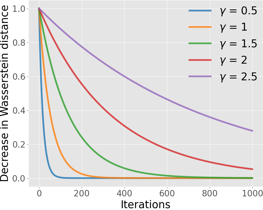
In Figure 1, we plot , the limiting decrease in the Wasserstein distance according to our upper bound, with varying values of the limiting ratio with the other remaining values in fixed. We observe that as this ratio increases, the number of iterations needed to approximately converge may still increase rather rapidly.
6 Final remarks
We studied the exact convergence behavior of the MHI sampler across general Wasserstein distances. We showed upper and lower bounds on the worst-case convergence rate for Wasserstein distances weaker than the total variation distance. We showed the exact convergence rate at every initialization for Wasserstein distances weaker than the total variation distance is the same and matches that of the total variation convergence rate [51]. When starting at a certain point, we gave exact convergence expressions. By centering an independent proposal, we directly imbue the Markov chain with a strong attraction to a set where the target distribution has high probability. We showed this technique can provide uniform control over acceptance probability yielding exact convergence rates in Bayesian quantile regression. The centered MHI sampler turns out to have many applications for posteriors that arise in Bayesian generalized linear models where more sophisticated proposals are often used. With additional assumptions on the data and prior, we also showed this exact convergence rate may be upper bounded when sampling high-dimensional posteriors in Bayesian binary response regression.
References
- [1] James H. Albert and Siddhartha Chib. Bayesian analysis of binary and polychotomous response data. Journal of the American Statistical Association, 88(422):669–679, 1993.
- [2] Alexandre Belloni and Victor Chernozhukov. On the computational complexity of MCMC-based estimators in large samples. The Annals of Statistics, 37(4):2011–2055, 2009.
- [3] Vladimir I. Bogachev. Gaussian Measures. American Mathematical Society, 1998.
- [4] Steve Brooks, Andrew Gelman, Galin L. Jones, and Xiao-Li Meng. Handbook of Markov chain Monte Carlo. Chapman and Hall/CRC, 1 edition, 2011.
- [5] Eugene Demidenko. Computational aspects of probit model. Mathematical Communications, 6:233–247, 2001.
- [6] Alain Durmus and Éric Moulines. Quantitative bounds of convergence for geometrically ergodic Markov chain in the Wasserstein distance with application to the Metropolis adjusted Langevin algorithm. Statistics and Computing, 25:5–19, 2015.
- [7] Alain Durmus and Éric Moulines. High-dimensional Bayesian inference via the unadjusted Langevin algorithm. Bernoulli, 25:2854–2882, 2019.
- [8] Raaz Dwivedi, Yuansi Chen, Martin J Wainwright, and Bin Yu. Log-concave sampling: Metropolis-Hastings algorithms are fast! In Proceedings of the 31st Conference On Learning Theory, volume 75 of Proceedings of Machine Learning Research, pages 793–797, 2018.
- [9] Andreas Eberle. Error bounds for Metropolis–Hastings algorithms applied to perturbations of Gaussian measures in high dimensions. The Annals of Applied Probability, 24(1):337 – 377, 2014.
- [10] Karl Oskar Ekvall and Galin L. Jones. Convergence analysis of a collapsed Gibbs sampler for Bayesian vector autoregressions. Electronic Journal of Statistics, 15:691–721, 2021.
- [11] Stuart Geman. A limit theorem for the norm of random matrices. The Annals of Probability, 8:252–261, 1980.
- [12] Alison L. Gibbs. Convergence in the Wasserstein metric for Markov chain Monte Carlo algorithms with applications to image restoration. Stochastic Models, 20(4):473–492, 2004.
- [13] Davide Giraudo. Product measure with a dirac delta marginal. Mathematics Stack Exchange, 2014.
- [14] Martin Hairer, Andrew M. Stuart, and Sebastian J. Vollmer. Spectral gaps for a Metropolis–Hastings algorithm in infinite dimensions. The Annals of Applied Probability, 24:2455–2490, 2014.
- [15] Wilfred K. Hastings. Monte Carlo sampling methods using Markov chains and their applications. Biometrika, 57:97–109, 1970.
- [16] Jean-Baptiste Hiriart-Urruty and Claude Lemaéchal. Fundamentals of Convex Analysis. Springer-Verlag Berlin Heidelberg, 1 edition, 2001.
- [17] Søren Fiig Jarner and Ernst Hansen. Geometric ergodicity of Metropolis algorithms. Stochastic Processes and their Applications, 85:341–361, 2000.
- [18] Rui Jin and Aixin Tan. Central limit theorems for Markov chains based on their convergence rates in Wasserstein distance. preprint arXiv:2002.09427, 2020.
- [19] James E. Johndrow, Aaron Smith, Natesh Pillai, and David B. Dunson. MCMC for imbalanced categorical data. Journal of the American Statistical Association, 114:1394–1403, 2019.
- [20] Leif T. Johnson and Charles J. Geyer. Variable transformation to obtain geometric ergodicity in the random-walk Metropolis algorithm. The Annals of Statistics, 40(6):3050 – 3076, 2012.
- [21] Galin L. Jones. On the Markov chain central limit theorem. Probability Surveys, 1:299–320, 2004.
- [22] Aldéric Joulin and Yann Ollivier. Curvature, concentration and error estimates for Markov chain Monte Carlo. The Annals of Probability, 38:2418–2442, 2010.
- [23] L. V. Kantorovich and G. S. Rubinstein. On a function space in certain extremal problems. Dokl. Akad. Nauk USSR, 115(6):1058–1061, 1957.
- [24] Kshitij Khare and James P. Hobert. Geometric ergodicity of the Gibbs sampler for Bayesian quantile regression. Journal of Multivariate Analysis, 112:108–116, 2012.
- [25] Tomasz Komorowski and Anna Walczuk. Central limit theorem for Markov processes with spectral gap in the Wasserstein metric. Stochastic Processes and their Applications, 122:2155–2184, 2011.
- [26] Jun S. Liu. Metropolized independent sampling with comparisons to rejection sampling and importance sampling. Statistics and Computing, 6(2):113–119, 1996.
- [27] Neal Madras and Deniz Sezer. Quantitative bounds for Markov chain convergence: Wasserstein and total variation distances. Bernoulli, 16(3):882 – 908, 2010.
- [28] Kerrie L. Mengersen and Richard L. Tweedie. Rates of convergence of the Hastings and Metropolis algorithms. The Annals of Statistics, 24:101–121, 1996.
- [29] Nicholas Metropolis, Arianna W. Rosenbluth, Marshall N. Rosenbluth, Augusta H. Teller, and Edward Teller. Equation of state calculations by fast computing machines. The Journal of Chemical Physics, 21:1087–1092, 1953.
- [30] Sean P. Meyn and Richard L. Tweedie. Markov Chains and Stochastic Stability. Cambridge University Press, USA, 2 edition, 2009.
- [31] Yurii Nesterov. Lectures on Convex Optimization. Springer International Publishing, 2 edition, 2018.
- [32] Omiros Papaspiliopoulos, Gareth O. Roberts, and Giacomo Zanella. Scalable inference for crossed random effects models. Biometrika, 107(1):25–40, 2019.
- [33] Omiros Papaspiliopoulos, Timothée Stumpf-Fétizon, and Giacomo Zanella. Scalable computation for Bayesian hierarchical models. preprint arXiv:2103.10875, 2021.
- [34] Jacob Pierre, Christian P. Robert, and Murray H. Smith. Using parallel computation to improve independent Metropolis–Hastings based estimation. Journal of Computational and Graphical Statistics, 20(3):616–635, 2011.
- [35] Nicholas G. Polson, James G. Scott, and Jesse Windle. Bayesian inference for logistic models using Pólya–Gamma latent variables. Journal of the American Statistical Association, 108:1339–1349, 2013.
- [36] Qian Qin and James P Hobert. Convergence complexity analysis of Albert and Chib’s algorithm for Bayesian probit regression. Annals of Statistics, 47:2320–2347, 2019.
- [37] Qian Qin and James P Hobert. Geometric convergence bounds for Markov chains in Wasserstein distance based on generalized drift and contraction conditions. To appear in Annales de l’Instute Henri Poincaré, 2021.
- [38] Qian Qin and James P Hobert. On the limitations of single-step drift and minorization in Markov chain convergence analysis. To appear in Annals of Applied Probability, 2021.
- [39] Qian Qin and James P Hobert. Wasserstein-based methods for convergence complexity analysis of MCMC with applications. To appear in Annals of Applied Probability, 2021.
- [40] Bala Rajaratnam and Doug Sparks. MCMC-based inference in the era of big data: A fundamental analysis of the convergence complexity of high-dimensional chains. preprint arXiv:1508.00947, 2015.
- [41] Gareth O. Roberts and Richard L. Tweedie. Geometric convergence and central limit theorems for multidimensional Hastings and Metropolis algorithms. Biometrika, 83:95–110, 1996.
- [42] Nathan Robertson, James M. Flegal, Dootika Vats, and Galin L. Jones. Assessing and visualizing simultaneous simulation error. Journal of Computational and Graphical Statistics, 30:324–334, 2021.
- [43] Jeffrey S. Rosenthal. Minorization conditions and convergence rates for Markov chain Monte Carlo. Journal of the American Statistical Association, 90:558–566, 1995.
- [44] Neil Shephard and Michael K. Pitt. Likelihood analysis of non-Gaussian measurement time series. Biometrika, 84(3):653–667, 1997.
- [45] Richard L Smith and Luke Tierney. Exact transition probabilities for the independence Metropolis sampler. Technical Report, 1996.
- [46] Pragya Sur and Emmanuel J. Candès. A modern maximum-likelihood theory for high-dimensional logistic regression. Proceedings of the National Academy of Sciences, 116:14516–14525, 2019.
- [47] Luke Tierney. Markov chains for exploring posterior distributions. The Annals of Statistics, 22:1701–1728, 1994.
- [48] Dootika Vats, James M. Flegal, and Galin L. Jones. Multivariate output analysis for Markov chain Monte Carlo. Biometrika, 106:321–337, 2019.
- [49] Cédric Villani. Topics in Optimal Transportation. Graduate studies in mathematics. American Mathematical Society, 2003.
- [50] Cédric Villani. Optimal Transport: Old and New. 338. Springer-Verlag Berlin Heidelberg, 1 edition, 2009.
- [51] Guanyang Wang. Exact convergence rate analysis of the independent Metropolis-Hastings algorithms. Bernoulli, 28:2012–2033, 2022.
- [52] Yun Yang, Martin J. Wainwright, and Michael I. Jordan. On the computational complexity of high-dimensional Bayesian variable selection. Annals of Statistics, 44:2497–2532, 2016.
Appendix A Proof of Theorem 1
The proof will proceed by establishing the upper and lower bounds separately in Lemmas 1 and 2, respectively. This is done largely because the conditions for the upper bound are weaker than those for the lower bound.
The following definitions will be used in the proofs of Lemmas 1 and 2. First, for , real-valued measurable functions , and a Markov kernel , we will use the notation and . Second, recall that for functions ,
Lemma 1.
Let . Then
Proof.
Let and let satisfy . The existence of implies the minorization condition [47, Corollary 4] which, in turn, ensures the residual kernel is a Markov kernel with invariant distribution . It then follows that
Since is Lipschitz with respect to , we then have
Taking the supremum with respect to and using the Kantorovich-Rubinstein theorem [49, Theorem 1.14],
∎
We now turn our attention to establishing the lower bound.
Lemma 2.
Let . Suppose is lower semicontinuous and is upper semicontinuous on . Suppose can be expressed as a countable union of compact sets. If , then
Proof.
Since can be expressed as a countable union of compact sets, there is a sequence of compact sets increasing to . We can assume or else we can take large enough so this holds. Since and is upper semicontinuous on , then is lower semicontinuous on . By Lemma 3, we have that is monotonically non-increasing to . Since we have assumed lower semicontinuity, the is attained over any compact set . Then define the sequence
| (14) |
We can then define the sequence
and this is monotonically non-increasing to .
Define to be the Metropolis-Hastings independence kernel with independent proposal with density and target distribution with density . By construction, and this is well-defined. The key part of the proof is that if we start at any , this kernel and the kernel only disagree outside of . For , we have , , and since by assumption, then . Also, if , then . Let be the set of measurable functions with . Therefore, for any and any function ,
Let . Since and are probability measures, we may then choose sufficiently large such that for all ,
We then have
| (15) |
Similarly,
| (16) |
With as in (14), let . Then for any ,
| (17) |
and . Since is invariant for the kernel ,
| (18) |
Now for any integer with , the function since is a Markov kernel. Since and , using (15), (16), and (18),
| (19) |
By construction of in (14), we have
For measurable [51, Remark 1, Theorem 2], we then have the identity
| (20) |
Since is a bounded measurable function, (20) gives the identity:
| (21) |
Using (19) in the first inequality, (21) in the second inequality, (16) in the third inequality, and using the invariance of for the Markov kernel in the last inequality,
Applying this inequality recursively and using the definition of
| (22) |
Since and , we may take large enough so that
For all large enough and since , we lower bound (22) to get
| (23) |
Combining (17) and (23), we lower bound the Wasserstein distance with
Since this holds for all small , the proof is complete by taking the limit as . ∎
Appendix B Technical Lemmas
Lemma 3.
Let . Suppose there is a sequence of compact sets increasing to . Define the sequence . Then is monotonically non-increasing to its limit .
Proof.
By definition of the infimum, and . Hence the sequence converges. Let . By the definition of the infimum, we can choose with such that
We can choose such that . Then
It follows that for any
Therefore, . ∎
Lemma 4.
Let be a positive-definite, symmetric matrix and . Let and suppose is convex for all points on . Then there exists and
Proof.
Since the function is convex for all points on , it follows that for any and any ,
Since is positive-definite, then is nonnegative and this implies that is a convex function. It can also be shown that and since is lower semicontinuous, then attains its minimum . The right directional derivative
exists for all points [31, Theorem 3.1.12]. For , we have
Taking the limit with , we have that
Since is the minimum of , then the right directional derivative satisfies for all . Therefore for all ,
∎