ColDE: A Depth Estimation Framework for Colonoscopy Reconstruction

ColDE: A Depth Estimation Framework for Colonoscopy Reconstruction

1 Introduction

2 Related Work

3 Methods

4 Experiments

5 Conclusion

References

Appendix A Results on KITTI Dataset

1 Introduction

2 Related Work

3 Methods

4 Experiments

5 Conclusion

References

Appendix A Results on KITTI Dataset

Appendix B Additional Results: Simulator Depth Maps Comparison

2.1 Monocular Depth Estimation

2.2 3D Reconstruction in Endoscopy

3.1 Photometric Objectives

3.2 Geometric Objectives

3.3 Training Overview

4.1 Implementation Details

4.2 Results on Colonoscopy Simulator Dataset

4.3 Results on Optical Colonoscopy Videos

4.4 Results on KITTI Dataset

2.1 Monocular Depth Estimation

2.2 3D Reconstruction in Endoscopy

3.1 Photometric Objectives

3.2 Geometric Objectives

3.3 Training Overview

4.1 Implementation Details

4.2 Results on Colonoscopy Simulator Dataset

4.3 Results on Optical Colonoscopy Videos

4.4 Results on KITTI Dataset

3.1.1 Appearance Similarity Objective

3.1.2 Feature Similarity Objective

3.2.1 Depth Consistency Objective

3.2.2 Normal Consistency Objective

4.2.1 Depth Prediction Errors and Accuracy

4.2.2 Ablation Study

4.3.1 3D Reconstruction Visualization

4.3.2 Expert Evaluation on Reconstruction Quality

3.1.1 Appearance Similarity Objective

3.1.2 Feature Similarity Objective

3.2.1 Depth Consistency Objective

3.2.2 Normal Consistency Objective

4.2.1 Depth Prediction Errors and Accuracy

4.2.2 Ablation Study

4.3.1 3D Reconstruction Visualization

4.3.2 Expert Evaluation on Reconstruction Quality

Surface Normal Prediction

Effect of masks

Effect of objectives

Limitations and future work

Acknowledgements

Surface Normal Prediction

Effect of masks

Effect of objectives

Limitations and future work

Acknowledgements

Abstract

Abstract

Yubo Zhang Affiliation: Department of Computer Science, University of North Carolina at Chapel Hill Jan-Michael Frahm Affiliation: Department of Computer Science, University of North Carolina at Chapel Hill Samuel Ehrenstein Affiliation: Department of Computer Science, University of North Carolina at Chapel Hill Sarah K. McGill Affiliation: Department of Medicine, University of North Carolina at Chapel Hill Julian G. Rosenman Affiliation: Department of Radiation Oncology, University of North Carolina at Chapel Hill{zhangyb,jmf,ehrensam,shuxian,pizer}@cs.unc.edumcgills@email.unc.edurosenmju@med.unc.edu Shuxian Wang Affiliation: Department of Computer Science, University of North Carolina at Chapel Hill Stephen M. Pizer Affiliation: Department of Computer Science, University of North Carolina at Chapel Hill

One of the key elements of reconstructing a 3D mesh from a monocular video is generating every frame’s depth map. However, in the application of colonoscopy video reconstruction, producing good-quality depth estimation is challenging. Neural networks can be easily fooled by photometric distractions or fail to capture the complex shape of the colon surface, predicting defective shapes that result in broken meshes. Aiming to fundamentally improve the depth estimation quality for colonoscopy 3D reconstruction, in this work we have designed a set of training losses to deal with the special challenges of colonoscopy data. For better training, a set of geometric consistency objectives was developed, using both depth and surface normal information. Also, the classic photometric loss was extended with feature matching to compensate for illumination noise. With the training losses powerful enough, our self-supervised framework named ColDE is able to produce better depth maps of colonoscopy data as compared to the previous work utilizing prior depth knowledge. Used in reconstruction, our network is able to reconstruct good-quality colon meshes in real-time without any post-processing, making it the first to be clinically applicable.

Refer to caption — Figure 1: Reconstructing the 3D mesh from a colonoscopy video in real-time according to the predicted depth and camera pose, allowing holes in the mesh to alert the physician to unsurveyed regions on the colon surface.

Colon cancer being one of the deadliest cancers worldwide, optical colonoscopy has been the most efficient for pre-cancerous screening. The procedure is operated by a physician, who controls a colonoscope inserted inside the patient’s large intestine (colon) and detects and removes lesions (polyps) that are visible on the live RGB video sent back from the scope. To increase the polyp detection rate, it is crucial to lowering the percentage of the colon surface that is missed from examination hong2007colonoscopy. As the unsurveyed regions are usually caused by the lack of camera orientations or occlusion by the colon structure itself, our approach is to reconstruct the already surveyed region from the colonoscopy video concurrently during the procedure so that the unsurveyed part can be reported to the physician as holes in the 3D surface (as in Fig. 1).

To reconstruct the 3D model from the monocular video, dense depth and camera pose transformation need to be predicted for each frame. Previous deep learning methods have been developed for that task in daily applications such as outdoor driving Geiger2012CVPR; cordts2016cityscapes and scene reconstruction saxena2008make3d; li2018megadepth. In most scenarios where ground-truth information is not available, photometric objectives have been proposed to train the network in a self-supervised fashion zhou2017unsupervised; zhan2018unsupervised. Later, additional geometric constraints have been explored bian2019unsupervised; yang2018lego; mahjourian2018unsupervised, and other visual clues such as optical flow yin2018geonet; ranjan2019competitive and segmentation casser2019depth; guizilini2019semantically have also been utilized to improve the performance. However, these approaches were primarily developed to estimate in the human-made world. Their validity to cope with colonoscopy data has not been fully studied, where the sparse texture and the poor illumination bring a great challenge to generate estimation, especially depth maps.

Due to the difficulty in estimation of the depth map directly from optical colonoscopy, previous work that dealt with the problem often used the help from prior knowledge available in virtual colonoscopy mathew2020augmenting or colon simulators zhang2020template; rau2019implicit. The first framework ma2019real; ma2021rnnslam that successfully reconstructed 3D models from real colonoscopy videos generated sparse pseudo ground-truth using structure-from-motion (SfM) schonberger2016structure so that the depth estimation network could be trained with semi-supervision. But even with the help of prior knowledge, the depth prediction was still vulnerable to environmental noise and failed to capture the surface information from time to time. When the depth predictions of frames were placed together to generate a 3D reconstruction mesh, their shapes were not aligned, causing a sparse and broken surface. To compensate, the authors introduced an additional averaging step and adjustment of the depth using SfM bae2020deep; liu2020reconstructing. However, these post-processing steps prevented the programs’ real-time execution.

In this work we introduce ColDE, a novel framework for Colonoscopy Depth Estimation, where we fundamentally improve the depth prediction quality for colonoscopy 3D reconstruction. Our contributions are the following:

•

We have designed our training losses to deal with the special challenges of colonoscopy data. A set of geometric consistency losses, constraining the surface’s 3D positions and normals, has been developed to enforce the shape consistency between frames. Also, the photometric loss has been extended with image feature matching, improving the network’s robustness to illumination change.
•

With these powerful training objectives, our framework is the first to be able to train the network in a fully self-supervised fashion from real colonoscopy videos without needing any prior knowledge.
•

When tested on the colon simulator data zhang2020template, our framework outperforms previous state-of-the-art monocular depth estimation methods on depth errors and accuracy.
•

Applied to optical colonoscopy data, our 3D reconstruction pipeline is the first to be clinically applicable, because it is able to generate depth maps in real-time that lead to meshes with desirable quality.

Here, we review the previous methods of estimating a depth map from a single RGB image and their use in reconstructing endoscopy videos.

Estimating the depth map of a single RGB image is an ill-posed problem. As deep learning has progressed, various networks and training methods have been developed to address the problem. When the ground-truth depth information is fully available, supervised training methods can lead to decent depth prediction eigen2015predicting; vijayanarasimhan2017sfm; fu2018deep. Others have explored the possibility to utilize sparse depth values obtained from sensors or other odometry approaches kuznietsov2017semi; yang2018deep.

However, acquiring the ground-truth depth information is challenging, so applying unsupervised training strategies is more applicable in some real-world scenarios. Godard et al. godard2017unsupervised proposed one of the earliest self-supervised approaches to generate depth maps from stereo images; then Zhou et al. zhou2017unsupervised extended the method and developed the first self-supervised monocular depth estimation framework. Later work explored various directions to improve the performance on outdoor Geiger2012CVPR; cordts2016cityscapes and indoor silberman2012indoor depth estimation tasks. Some focused on solving specific issues that often occur in training and at test time, e.g., the scale inconsistency issue wang2018learning; xiong2020self; ji2021monoindoor and the mixed information brought in by independent motion or static frames monodepth2; bian2019unsupervised; li2020unsupervised. Better network architectures have been proposed packnet; zou2020learning; lyu2020hr; you2021towards. Additional training objectives that extend the photometric constraint zhan2018unsupervised; yang2018unsupervised or introduce geometric constraints yang2018unsupervised; yang2018lego; mahjourian2018unsupervised; bian2019unsupervised; li2021structdepth have been found useful. Other visual information, such as optical flow yin2018geonet; zou2018df; ranjan2019competitive and semantic segmentation casser2019depth; meng2019signet; guizilini2019semantically, were also utilized to help the depth estimation.

Applying monocular depth estimation to endoscopy data, such as optical colonoscopy, is challenging due to the low-texture surface and the complex lighting. As pure self-supervised methods may struggle to complete the task, previous work tried to augment the training data with ground-truth depth information, which is only fully available in virtual colonoscopy. In order to transfer the knowledge learned from synthetic data to real data, several methods mahmood2018unsupervised; mathew2020augmenting; cheng2021depth made use of GAN frameworks and Itoh et al. itoh2021unsupervised designed a reflection model.

In the work by Ma et al. ma2019real; ma2021rnnslam, with the help of structure-from-motion (SfM) schonberger2016structure to generate sparse depth information, the depth estimation network wang2019recurrent was trained in a semi-supervised fashion with only real data. Then accompanied by a SLAM system engel2017direct to predict camera poses, they developed the first framework that was able to reconstruct colon meshes from colonoscopy videos in real-time. However, their depth estimation network can only handle simple cases and is vulnerable to environmental noise, and the predicted shapes often fail to produce good quality meshes. Later work bae2020deep; liu2020reconstructing exploited the possibility to integrate SfM with the learning-based depth estimation to calibrate depth predictions, but the time expense brought in by SfM restricts the methods from large-scale reconstruction applications.

To improve these endoscopy reconstruction prototypes, in this work we target their weak link, which is the neural depth estimation component. Using only the optical (RGB) colonoscopy data available, we aim to substantially improve the effectiveness and efficiency of the reconstruction by a better training strategy.

In most of the previous monocular depth estimation frameworks zhou2017unsupervised; monodepth2; bian2019unsupervised, the self-supervision signals that train the network come from the projection relation between a source view $s$ and a target view $t$ . Given the camera intrinsic $K$ , a pixel $p_{t}$ in a target view can be projected into the source view according to the predicted depth map $\hat{D}_{t}$ and the relative camera transformation $\hat{T}_{t\to s}$ . This process yields the pixel’s homogeneous coordinates $\hat{p}_{s}$ and its projected depth $\hat{d}_{s}^{t}$ in the source view, as in Eq. 1:

\displaystyle\hat{p}_{s},\hat{d}^{t}_{s}\sim K\hat{T}_{t\to s}\hat{D}_{t}(p_{t})K^{-1}p_{t}

(1)

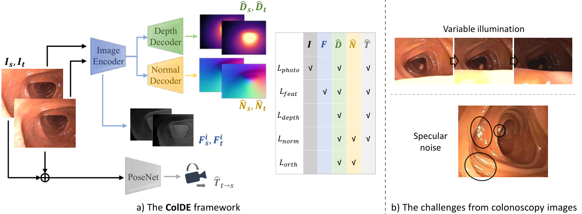
Here, we describe our colonoscopy depth estimation framework shown in Fig. 2 a. Building upon the projection relation in Eq. 1, we construct a set of self-supervised photometric and geometric objectives, which target the colonoscopy video reconstruction task that is challenging due to lighting complexity and complicated topology. These objectives are used to train the depth and pose estimation networks; details will be discussed later in this section.

The first set of training objectives is based on the photometric information. We will first discuss using the RGB image appearance as the objective and then using feature maps.

Based on the projection in Eq. 1, the source image $I_{s}$ can be warped into the target view $I_{t}$ as in Eq. 2, where $\left\langle*\right\rangle$ denotes bilinear interpolation. Assuming the scene is rigid and the light source does not change much, which is the case for most of a colonoscopy video, the warped source image $\hat{I}_{s}$ should agree with the target image, so with the appearance difference we formulate the photometric similarity objective $L_{photo}$ to supervise the depth and camera pose training, as in Eq. 3. $\rm SSIM(*,*)$ denotes the structural similarity measurement wang2004image. Following godard2017unsupervised; monodepth2 we set $\alpha=0.85$ .

	$\displaystyle\hat{I}_{s}=I_{s}\left\langle\hat{p}_{s}\right\rangle$		(2)
	$\displaystyle L_{photo}=(1-\alpha)\|\|\hat{I}_{s}-I_{t}\|\|_{1}+\frac{\alpha}{2}(1-{\rm SSIM}(\hat{I}_{s},I_{t}))$		(3)

Trained with only the appearance clue (image intensity), the neural network can be vulnerable to photometric variation in the environment. In colonoscopy videos the light source is moving with the camera and obstacles often occur to block the lumination, leading to changing contrast and brightness zhang2021lighting. Moreover, the watery surface can reflect the light and cause notable specular noise, as shown in Fig. 2 b.

To deal with this issue, in addition to the appearance-based photometric loss, we have designed a feature-based similarity objective zhan2018unsupervised. We utilize the early features from the depth prediction network (conv $1$ output of ResNet encoder he2016deep), which represent local semantic information. In each training iteration, we randomly sample one feature map out of $64$ to be used as the source and target “images”, $F^{i}_{s}$ and $F^{i}_{t}$ , and the feature similarity objective $L_{feat}$ is constructed with the target and warped source feature maps as

\displaystyle L_{feat}=\frac{\alpha}{2}(1-{\rm SSIM}(F^{i}_{s}\left\langle\hat{p}_{s}\right\rangle,F^{i}_{t})),i\ {\rm in}\left\{1,...,64\right\}

(4)

Here we only include the semantics-communicating structural similarity term in feature matching. Additionally, during training $L_{feat}$ directly supervises the first step of feature extraction, further making the process robust to variable lighting.

The network trained with photometric objectives may seem to produce decent depth maps for individual images. But when they are stitched together to produce the overall 3D model of the scene, the projected shapes of adjacent frames may not align with each other, causing defective reconstruction ma2021rnnslam. To cope with this issue, we design another set of training objectives to enforce geometric consistency, specifically, on 3D positions and surface normals.

Directly measuring the geometric consistency between two shapes is not easy mahjourian2018unsupervised, so instead we measure the difference between the predicted depths of the same scene in different frames. According to Eq. 1, each vertex in the predicted 3D shape of the target frame (derived from $\hat{D}_{t}$ ) has the depth of $\hat{d}^{t}_{s}$ relative to the source view’s camera. Meanwhile, the network can also produce a depth map $\hat{D}_{s}$ for the source image. As the predicted depth of the source image should agree with the projected depth from the target image, we can construct a depth consistency objective as in Eq. 5, in which we adopt the means in bian2019unsupervised to normalize the depth:

\displaystyle L_{depth}=\frac{\left|\hat{D}_{s}\left\langle\hat{p}_{s}\right\rangle-\hat{D}^{t}_{s}\right|}{\hat{D}_{s}\left\langle\hat{p}_{s}\right\rangle+\hat{D}^{t}_{s}}

(5)

With the depth consistency enforced, when projecting images into the 3D space, the 3D models from the target and source views will be better aligned and can be stitched together closely.

Surface normals provide useful information about objects’ shape yang2018unsupervised. It describes the orientation of the 3D surface and reflects local shape knowledge. As the derivative of vertices’ 3D positions, they can be sensitive to the error and noise on the predicted surface. Therefore, utilizing surface normal correspondence during training can further correct the network prediction and improve the shape consistency.

Let $\hat{N}_{t}$ be the object’s surface normals in the target coordinate system. Then in the source view’s coordinate system those vectors will be in different directions depending on the relative camera rotation $\hat{R}_{t\to s}$ (the rotation component of $\hat{T}_{t\to s}$ ). These directions from the target view should agree with the source view’s own normal prediction $\hat{N}_{s}$ ; using this correspondence we form the normal consistency objective as

\displaystyle L_{norm}=||\hat{N}_{s}\left\langle\hat{p}_{s}\right\rangle-\hat{R}_{t\to s}\hat{N}_{t}||_{1}

(6)

Here, we simply use the numerical difference between the two vectors to compute the normal error. In practice, we find that using angular difference has similar performance.

Previous practice often obtained normal vectors by computing the mean cross product of surface vector prediction yang2018unsupervised; yang2018lego. However, we found that when training with colonoscopy data, computing normals directly from depths is less stable and tends to result in unrealistic shapes, since the colon surface is less flat compared to the surfaces in human-made worlds. Instead, we apply a separate decoder to predict surface normal information. The normal decoder has almost the same architecture as the depth decoder, only with a different number of output channels, and two decoders share the same image encoder, as shown in Fig 2 a. To bridge the depth and normal predictions, we further apply an orthogonality constraint:

	$\displaystyle\hat{V}(p)=\hat{D}(p_{a})K^{-1}p_{a}-\hat{D}(p_{b})K^{-1}p_{b}$		(7)
	$\displaystyle L_{orth}=\sum_{p}\hat{N}(p)\cdot\hat{V}(p)$		(8)

where $\hat{V}(p)$ is the approximate surface vector around $p$ , which is computed from the depths of $p_{a}$ and $p_{b}$ , $p$ ’s nearby pixels. In practice, we apply two pairs of $p_{a/b}$ position combinations, i.e., $p$ ’s top-left/bottom-right pixels and top-right/bottom-left pixels.

Apart from the photometric and geometric objectives discussed above, we follow the previous work godard2017unsupervised and include an edge-aware smoothness prior $L_{sm}$ , which is applied to both source and target views’ depth predictions. But in contrast to previous work zhan2019self, we have not found it useful to include a normal smoothness prior, since normal orientations of the colon surface do not necessarily follow the intensity clue in colonoscopy images.

To mask out the pixels of stationary frames in colonoscopy training sequences, we follow the auto-masking scheme in monodepth2 applying a mask $M_{auto}$ . We also follow ma2021rnnslam to add a specular mask $M_{spec}$ to mask out specular regions. Additionally, a valid mask $M_{valid}$ is applied to exclude the pixels that would be warped outside of the source view. So the overall mask to select pixels in consistency objectives is the combination of three masks mentioned above, where $\odot$ denotes element-wise production:

\displaystyle M=M_{auto}\odot M_{spec}\odot M_{valid}

(9)

Summing up all the elements, the training loss to supervise the network is written as Eq. 10, where $\lambda_{1}$ - $\lambda_{5}$ are the weights of each objective.

	$\displaystyle L=$	$\displaystyle(L_{photo}+\lambda_{1}L_{feat}+\lambda_{2}L_{depth}+\lambda_{3}L_{norm})\odot M$		(10)
		$\displaystyle+\lambda_{4}L_{orth}+\lambda_{5}L_{sm}$		(10)

We validated our ColDE framework on colon simulator data and real optical colonoscopy videos. We also tested our method on the KITTI dataset. The results are analyzed in this section.

We constructed our networks following monodepth2. Due to the time efficiency concern, our image encoder is built with ResNet18 he2016deep, which has relatively few parameters. As in Fig. 2 a, the image encoder takes a single RGB image as the input, and the encoded image features are given to depth and normal decoders that respectively produce depth and normal maps. The PoseNet takes a pair of images and produces their relative $6$ D camera transformation. In our experiments all input RGB images are resized to $224\times 288$ .

We used the pre-training and fine-tuning training scheme to train the network in the following experiments. In the pre-training steps, the learning rate was set at $10^{-4}$ . First, $\lambda_{3,4}$ were set to be $0$ in Eq. 10, and we trained the image encoder, depth decoder and PoseNet with $\lambda_{1}=0.1$ , $\lambda_{2}=0.1$ and $\lambda_{5}=0.01$ for $20$ epochs. Then the above three modules were frozen, and we trained the normal decoder alone for $20$ epochs with $\lambda_{3}=0.1$ and $\lambda_{4}=0.5$ . Finally, all modules were fine-tuned together for $10$ epochs with learning rate $10^{-5}$ . The weights for fine-tuning were $\lambda_{1}=0.1$ , $\lambda_{2}=0.1$ , $\lambda_{3}=0.005$ , $\lambda_{4}=0.001$ and $\lambda_{5}=0.01$ .

We first tested our method on the synthetic data from a colon simulator zhang2020template. In that simulator a pre-defined 3D colon model is rendered with textures similar to optical colonoscopy videos but with less specular reflection. As a simulated colonoscope traveling inside the colon, the RGB image and the ground-truth depth are saved for each frame. In our experiments our data comes from $9$ simulated colonoscopy videos generated by this program, from which we randomly sampled training/validation/testing sets that contain $9.5$ k/ $0.5$ k/ $2.5$ k frames. The accuracies reported below are the results on the testing split.

Methods	Error metric $\downarrow$				Accuracy metric $\uparrow$			Speed $\uparrow$
Methods	Abs Rel	Sq Rel	RMSE	RMSE log	$\delta<1.25$	$\delta<1.25^{2}$	$\delta<1.25^{3}$	FPS
SfMLearner zhou2017unsupervised	0.276	0.832	1.592	0.333	0.660	0.881	0.947	26
SC-SfMLearner bian2019unsupervised	0.108	0.132	0.906	0.171	0.874	0.957	0.983	35
Monodepth2 monodepth2	0.097	0.110	0.811	0.154	0.913	0.971	0.987	36
PackNet-SfM packnet	0.101	0.106	0.792	0.152	0.901	0.968	0.988	2
HR-Depth lyu2020hr	0.096	0.109	0.813	0.153	0.913	0.971	0.987	22
ColDE	0.077	0.079	0.701	0.134	0.935	0.975	0.989	36

Table 1: Quantitative results (errors and accuracy) on colonoscopy simulator data. All results were produced from the networks trained with only self-supervised losses. The best result of each category is in bold and the second best is underlined. Our method ColDE outperforms previous monocular depth estimation methods on error and accuracy measures, while achieving real-time execution.

In Table 1 we list the depth prediction results of our ColDE framework and other state-of-the-art monocular depth estimation methods. For a fair comparison, only the self-supervised training objectives of these approaches were applied, and the trainings were conducted using the same training split of the simulator data described above. When evaluated, the depth prediction of each frame was re-scaled to the median ground-truth, as in monodepth2.

The results on the colonoscopy data show that our framework outperforms previous state-of-the-art methods that had been designed to give high accuracy for outdoor driving. Due to our real-time requirement, we also measured the execution speed of each approach. When running on a single Nvidia Quadro RTX5000 GPU, our network generated depth maps at $36$ frames-per-second (fps), well faster than the colonoscopy video speed of about $20$ fps.

To visually compare the depth quality, in Fig. 3 we show the depth map predictions from our method and from several previous works. Overall, our approach produced smooth depths on the colon surface while maintaining sharp boundaries around haustral folds, resembling the colon shape in real-world and ground-truth depth maps. Moreover, the other methods were vulnerable to visual distractions. For example in the third case of Fig. 3, their depths were discontinuous around the specular regions on the image’s top-left, near the haustral folds. In the fourth case, the blood vessel texture on the top-left part of the image distracted the networks monodepth2; lyu2020hr, resulting in unrealistic depth fluctuations.

Ablation		Error metric $\downarrow$				Accuracy metric $\uparrow$
Ablation		Abs Rel	Sq Rel	RMSE	RMSE log	$\delta<1.25$	$\delta<1.25^{2}$	$\delta<1.25^{3}$	#
Masks	Baseline ( $M$ )	0.087	0.094	0.745	0.144	0.924	0.972	0.987	1
	$-M_{spec}$	0.085	0.091	0.735	0.142	0.928	0.973	0.988	2
	$-M_{spec,valid}$	0.093	0.099	0.764	0.149	0.918	0.971	0.988	3
Losses	Baseline ( $L_{photo}$ )	0.087	0.094	0.745	0.144	0.924	0.972	0.987	4
	$+L_{feat}$	0.085	0.091	0.737	0.143	0.925	0.971	0.987	5
	$+L_{feat,depth}$	0.082	0.084	0.710	0.138	0.927	0.973	0.988	6
	$+L_{feat,depth,norm}$	0.077	0.079	0.701	0.134	0.935	0.975	0.989	7

Table 2: Ablation study. The effect of different masking schemes is shown in the first section. Although the specular mask improves depth quality visually, it has little impact on errors and accuracy; while the valid mask significantly improves performance. The impact of training objectives is shown in the second section. Our additional feature consistency loss and geometric losses can improve the depth quality.

We study the effect of every mask and loss component in our framework. Starting with the baseline model that is trained with only the appearance similarity objective $L_{photo}$ but with all masks $M$ applied, we gradually applied more objectives or eliminated mask components and studied the performance; the results are shown in Table 2.

As the specular mask is primarily to eliminate the effect of specular noise that is more common in optical colonoscopy ma2021rnnslam, we found that $M_{spec}$ did not show benefit on error or accuracy improvement on the simulator dataset (comparing line $2$ to $1$ in Table 2). Meanwhile, the valid mask is proven to be beneficial, as the errors significantly increased and accuracy decreased when we removed $M_{valid}$ from training between line $2$ and $3$ .

In the second part of Table 2, we analyzed the effect of different loss functions. After adding the feature consistency objective into the photometric losses, line $5$ shows improved depth quality. The biggest improvement is provided by the geometric constraints. In line $6$ and $7$ the errors drop significantly when $L_{depth}$ is added, and the accuracy has a substantial improvement after $L_{norm}$ is used. Although the primary purpose of including geometric objectives is to improve the depth consistency between frames, they strengthen the network’s ability to interpret shape information and thereby generate better depth maps for single images.

To test our method on optical colonoscopy data, we selected videos from $85$ clinical procedures, where each video contains about $20$ k frames. From those videos we manually selected $79$ video clips in which the camera was in a moderate pulling back or pushing forward movement. These testing sequences have $60$ to $300$ frames with an average of about $150$ . Additionally, we randomly sampled $185$ k frames from the rest of the videos and used them and their adjacent frames to train the network; another $5$ k-frame set was sampled for validation.

Testing predicted depth maps of optical colonoscopy data requires reconstructing 3D meshes. We adopted the system in ma2021rnnslam, where a SLAM component engel2017direct calculates corrected camera poses using the neural network’s depth output and then a fusion component uses these poses to stitch the shapes of the frames together. All the results reported below were generated with this system, but with the depth prediction network from the cited approaches. The reconstruction system also provides a post-processing option named “windowed depth averaging” that averages the shapes of adjacent frames, eliminating outliers but sacrificing the real-time execution. For comparison, we will show the reconstruction results with this post-processing step (with window size $7$ as in ma2021rnnslam), along with the ones without.

Fig. 4 visualizes the reconstruction results of $3$ cases from our approach and previous works. The results from ma2021rnnslam were produced using their pre-trained network, which was trained with semi-supervision from real colonoscopy data, while the models of monodepth2 and ColDE were trained with our optical colonoscopy dataset. Apart from the full model, we also show one ablation of our method that only included one geometric objective, corresponding to line $6$ in Table 2.

Our model (the last column) is the only one to be able to reconstruct colon surfaces with good quality without using averaging post-processing; excluding the normal consistency loss deteriorates the result (penultimate column). The common problem with other approaches is that their reconstructed surfaces are often sparse and broken due to shape misalignment among frames, thereby requiring averaging. Moreover, when the shape information is not fully captured, artifacts with a “skirt” shape can occur around colon cylinders, as seen in “without averaging” results in columns $1$ and $3$ of Fig. 4. However, these artifacts are less common in our full approach, as the network interprets shapes better when trained with geometric constraints.

We conducted human evaluation of the reconstruction quality of $79$ testing sequences. As instructed and verified by a colonoscopist, a member of our team judged the informativeness of the reconstructed meshes. Reconstruction with the following characteristics is considered ideal: 1) the overall shape is similar to a generalized cylinder that resembles a human colon; 2) the mesh contains few outliers and noise; 3) the surface has little unrealistic sparsity. Based on the above standard, reconstruction quality was categorized into three categories, i.e., “good”, “moderate” and “poor”.

Methods		Number of cases
Methods		Good	Moderate	Poor
w/ ave	RNNSLAM ma2021rnnslam	44	27	8
	ColDE ( $-L_{norm}$ )	57	16	6
	ColDE (full)	62	13	4
w/o ave	RNNSLAM ma2021rnnslam	34	34	11
	ColDE ( $-L_{norm}$ )	38	26	15
	ColDE (full)	62	13	4

Table 3: Expert evaluation on the reconstruction quality. Our full model can produce more “good” meshes than the indicated alternatives.

As compared to the previous colonoscopy reconstruction approach ma2021rnnslam and our ablation, the categorization results in Table 3 show that our framework produced notably more “good” reconstructions even without using windowed depth averaging. Although the averaging post-processing can slightly change the sparsity of the mesh surface produced by our model as shown in Fig. 4, it is seen to have little effect on the overall quality by category. Importantly, it indicates that our method can capture the colon shape well enough to make the geometry post-processing unnecessary.

As detailed in the supplementary material, our method is competitive to the best of the published alternatives on the KITTI outdoor driving dataset Geiger2012CVPR.

Aiming to fundamentally improve the depth estimation quality of colonoscopy images, in this work we developed a set of training objectives to cope with their special challenges. Geometric losses were designed to capture colon shape information and the photometric loss was extended to compensate noise. Applied to colonoscopy video reconstruction, our network trained without any supervision is the first to be able to produce good-quality 3D meshes without post-processing, making the system clinically applicable.

Although our approach brought significant improvement on colonoscopy depth estimation, there are still situations where the image illumination and texture are too complicated for our framework to handle. For example, there is one category of our failures that we call the “en face” situation, where the camera directly faces the low-texture colon surface, confusing the current network. To further improve the performance, optical flow may be useful to be included in the training, and the network architecture can be improved or re-designed to utilize temporal information. We leave these further explorations to future work.

We are grateful for the support from Shuai Zhang and his team for the use of their colonoscopy simulator. We thank Olympus, Inc. for their funding and Zhen Li and his team at Olympus for their advice.

(1) Gwangbin Bae, Ignas Budvytis, Chung-Kwong Yeung, and Roberto Cipolla. Deep multi-view stereo for dense 3d reconstruction from monocular endoscopic video. In International Conference on Medical Image Computing and Computer-Assisted Intervention, pages 774–783. Springer, 2020.
(2) Jiawang Bian, Zhichao Li, Naiyan Wang, Huangying Zhan, Chunhua Shen, Ming-Ming Cheng, and Ian Reid. Unsupervised scale-consistent depth and ego-motion learning from monocular video. Advances in neural information processing systems, 32:35–45, 2019.
(3) Vincent Casser, Soeren Pirk, Reza Mahjourian, and Anelia Angelova. Depth prediction without the sensors: Leveraging structure for unsupervised learning from monocular videos. In Proceedings of the AAAI conference on artificial intelligence, volume 33, pages 8001–8008, 2019.
(4) Kai Cheng, Yiting Ma, Bin Sun, Yang Li, and Xuejin Chen. Depth estimation for colonoscopy images with self-supervised learning from videos. In International Conference on Medical Image Computing and Computer-Assisted Intervention, pages 119–128. Springer, 2021.
(5) Marius Cordts, Mohamed Omran, Sebastian Ramos, Timo Rehfeld, Markus Enzweiler, Rodrigo Benenson, Uwe Franke, Stefan Roth, and Bernt Schiele. The cityscapes dataset for semantic urban scene understanding. In Proceedings of the IEEE conference on computer vision and pattern recognition, pages 3213–3223, 2016.
(6) David Eigen and Rob Fergus. Predicting depth, surface normals and semantic labels with a common multi-scale convolutional architecture. In Proceedings of the IEEE international conference on computer vision, pages 2650–2658, 2015.
(7) Jakob Engel, Vladlen Koltun, and Daniel Cremers. Direct sparse odometry. IEEE transactions on pattern analysis and machine intelligence, 40(3):611–625, 2017.
(8) Huan Fu, Mingming Gong, Chaohui Wang, Kayhan Batmanghelich, and Dacheng Tao. Deep ordinal regression network for monocular depth estimation. In Proceedings of the IEEE conference on computer vision and pattern recognition, pages 2002–2011, 2018.
(9) Andreas Geiger, Philip Lenz, and Raquel Urtasun. Are we ready for autonomous driving? the kitti vision benchmark suite. In Conference on Computer Vision and Pattern Recognition (CVPR), 2012.
(10) Clément Godard, Oisin Mac Aodha, and Gabriel J Brostow. Unsupervised monocular depth estimation with left-right consistency. In Proceedings of the IEEE conference on computer vision and pattern recognition, pages 270–279, 2017.
(11) Clément Godard, Oisin Mac Aodha, Michael Firman, and Gabriel J Brostow. Digging into self-supervised monocular depth estimation. In Proceedings of the IEEE/CVF International Conference on Computer Vision, pages 3828–3838, 2019.
(12) Vitor Guizilini, Rares Ambrus, Sudeep Pillai, Allan Raventos, and Adrien Gaidon. 3d packing for self-supervised monocular depth estimation. In IEEE Conference on Computer Vision and Pattern Recognition (CVPR), 2020.
(13) Vitor Guizilini, Rui Hou, Jie Li, Rares Ambrus, and Adrien Gaidon. Semantically-guided representation learning for self-supervised monocular depth. In International Conference on Learning Representations, 2019.
(14) Kaiming He, Xiangyu Zhang, Shaoqing Ren, and Jian Sun. Deep residual learning for image recognition. In Proceedings of the IEEE conference on computer vision and pattern recognition, pages 770–778, 2016.
(15) Wei Hong, Jianning Wang, Feng Qiu, Arie Kaufman, and Joseph Anderson. Colonoscopy simulation. In Medical Imaging 2007: Physiology, Function, and Structure from Medical Images, volume 6511, page 65110R. International Society for Optics and Photonics, 2007.
(16) Hayato Itoh, Masahiro Oda, Yuichi Mori, Masashi Misawa, Shin-Ei Kudo, Kenichiro Imai, Sayo Ito, Kinichi Hotta, Hirotsugu Takabatake, Masaki Mori, et al. Unsupervised colonoscopic depth estimation by domain translations with a lambertian-reflection keeping auxiliary task. International Journal of Computer Assisted Radiology and Surgery, 16(6):989–1001, 2021.
(17) Pan Ji, Runze Li, Bir Bhanu, and Yi Xu. Monoindoor: Towards good practice of self-supervised monocular depth estimation for indoor environments. In Proceedings of the IEEE/CVF International Conference on Computer Vision, pages 12787–12796, 2021.
(18) Yevhen Kuznietsov, Jorg Stuckler, and Bastian Leibe. Semi-supervised deep learning for monocular depth map prediction. In Proceedings of the IEEE conference on computer vision and pattern recognition, pages 6647–6655, 2017.
(19) Boying Li, Yuan Huang, Zeyu Liu, Danping Zou, and Wenxian Yu. Structdepth: Leveraging the structural regularities for self-supervised indoor depth estimation. In Proceedings of the IEEE/CVF International Conference on Computer Vision, pages 12663–12673, 2021.
(20) Hanhan Li, Ariel Gordon, Hang Zhao, Vincent Casser, and Anelia Angelova. Unsupervised monocular depth learning in dynamic scenes. 4th Conference on Robot Learning (CoRL), 2020.
(21) Zhengqi Li and Noah Snavely. Megadepth: Learning single-view depth prediction from internet photos. In Proceedings of the IEEE Conference on Computer Vision and Pattern Recognition, pages 2041–2050, 2018.
(22) Xingtong Liu, Maia Stiber, Jindan Huang, Masaru Ishii, Gregory D Hager, Russell H Taylor, and Mathias Unberath. Reconstructing sinus anatomy from endoscopic video–towards a radiation-free approach for quantitative longitudinal assessment. In International Conference on Medical Image Computing and Computer-Assisted Intervention, pages 3–13. Springer, 2020.
(23) Xiaoyang Lyu, Liang Liu, Mengmeng Wang, Xin Kong, Lina Liu, Yong Liu, Xinxin Chen, and Yi Yuan. Hr-depth: high resolution self-supervised monocular depth estimation. CoRR abs/2012.07356, 2020.
(24) Ruibin Ma, Rui Wang, Stephen Pizer, Julian Rosenman, Sarah K McGill, and Jan-Michael Frahm. Real-time 3d reconstruction of colonoscopic surfaces for determining missing regions. In International Conference on Medical Image Computing and Computer-Assisted Intervention, pages 573–582. Springer, 2019.
(25) Ruibin Ma, Rui Wang, Yubo Zhang, Stephen Pizer, Sarah K McGill, Julian Rosenman, and Jan-Michael Frahm. Rnnslam: Reconstructing the 3d colon to visualize missing regions during a colonoscopy. Medical image analysis, 72:102100, 2021.
(26) Reza Mahjourian, Martin Wicke, and Anelia Angelova. Unsupervised learning of depth and ego-motion from monocular video using 3d geometric constraints. In Proceedings of the IEEE Conference on Computer Vision and Pattern Recognition, pages 5667–5675, 2018.
(27) Faisal Mahmood, Richard Chen, and Nicholas J Durr. Unsupervised reverse domain adaptation for synthetic medical images via adversarial training. IEEE transactions on medical imaging, 37(12):2572–2581, 2018.
(28) Shawn Mathew, Saad Nadeem, Sruti Kumari, and Arie Kaufman. Augmenting colonoscopy using extended and directional cyclegan for lossy image translation. In Proceedings of the IEEE/CVF Conference on Computer Vision and Pattern Recognition, pages 4696–4705, 2020.
(29) Yue Meng, Yongxi Lu, Aman Raj, Samuel Sunarjo, Rui Guo, Tara Javidi, Gaurav Bansal, and Dinesh Bharadia. Signet: Semantic instance aided unsupervised 3d geometry perception. In Proceedings of the IEEE/CVF Conference on Computer Vision and Pattern Recognition, pages 9810–9820, 2019.
(30) Anurag Ranjan, Varun Jampani, Lukas Balles, Kihwan Kim, Deqing Sun, Jonas Wulff, and Michael J Black. Competitive collaboration: Joint unsupervised learning of depth, camera motion, optical flow and motion segmentation. In Proceedings of the IEEE/CVF Conference on Computer Vision and Pattern Recognition, pages 12240–12249, 2019.
(31) Anita Rau, PJ Eddie Edwards, Omer F Ahmad, Paul Riordan, Mirek Janatka, Laurence B Lovat, and Danail Stoyanov. Implicit domain adaptation with conditional generative adversarial networks for depth prediction in endoscopy. International journal of computer assisted radiology and surgery, 14(7):1167–1176, 2019.
(32) Ashutosh Saxena, Min Sun, and Andrew Y Ng. Make3d: Learning 3d scene structure from a single still image. IEEE transactions on pattern analysis and machine intelligence, 31(5):824–840, 2008.
(33) Johannes L Schonberger and Jan-Michael Frahm. Structure-from-motion revisited. In Proceedings of the IEEE conference on computer vision and pattern recognition, pages 4104–4113, 2016.
(34) Nathan Silberman, Derek Hoiem, Pushmeet Kohli, and Rob Fergus. Indoor segmentation and support inference from rgbd images. In European conference on computer vision, pages 746–760. Springer, 2012.
(35) Sudheendra Vijayanarasimhan, Susanna Ricco, Cordelia Schmid, Rahul Sukthankar, and Katerina Fragkiadaki. Sfm-net: Learning of structure and motion from video. arXiv preprint arXiv:1704.07804, 2017.
(36) Chaoyang Wang, José Miguel Buenaposada, Rui Zhu, and Simon Lucey. Learning depth from monocular videos using direct methods. In Proceedings of the IEEE Conference on Computer Vision and Pattern Recognition, pages 2022–2030, 2018.
(37) Rui Wang, Stephen M Pizer, and Jan-Michael Frahm. Recurrent neural network for (un-) supervised learning of monocular video visual odometry and depth. In Proceedings of the IEEE/CVF Conference on Computer Vision and Pattern Recognition, pages 5555–5564, 2019.
(38) Zhou Wang, Alan C Bovik, Hamid R Sheikh, and Eero P Simoncelli. Image quality assessment: from error visibility to structural similarity. IEEE transactions on image processing, 13(4):600–612, 2004.
(39) Mingkang Xiong, Zhenghong Zhang, Weilin Zhong, Jinsheng Ji, Jiyuan Liu, and Huilin Xiong. Self-supervised monocular depth and visual odometry learning with scale-consistent geometric constraints. In IJCAI, pages 963–969, 2020.
(40) Nan Yang, Rui Wang, Jorg Stuckler, and Daniel Cremers. Deep virtual stereo odometry: Leveraging deep depth prediction for monocular direct sparse odometry. In Proceedings of the European Conference on Computer Vision (ECCV), pages 817–833, 2018.
(41) Zhenheng Yang, Peng Wang, Yang Wang, Wei Xu, and Ram Nevatia. Lego: Learning edge with geometry all at once by watching videos. In Proceedings of the IEEE conference on computer vision and pattern recognition, pages 225–234, 2018.
(42) Zhenheng Yang, Peng Wang, Wei Xu, Liang Zhao, and Ramakant Nevatia. Unsupervised learning of geometry from videos with edge-aware depth-normal consistency. In Thirty-Second AAAI conference on artificial intelligence, 2018.
(43) Zhichao Yin and Jianping Shi. Geonet: Unsupervised learning of dense depth, optical flow and camera pose. In Proceedings of the IEEE conference on computer vision and pattern recognition, pages 1983–1992, 2018.
(44) Zunzhi You, Yi-Hsuan Tsai, Wei-Chen Chiu, and Guanbin Li. Towards interpretable deep networks for monocular depth estimation. In Proceedings of the IEEE/CVF International Conference on Computer Vision, pages 12879–12888, 2021.
(45) Huangying Zhan, Ravi Garg, Chamara Saroj Weerasekera, Kejie Li, Harsh Agarwal, and Ian Reid. Unsupervised learning of monocular depth estimation and visual odometry with deep feature reconstruction. In Proceedings of the IEEE conference on computer vision and pattern recognition, pages 340–349, 2018.
(46) Huangying Zhan, Chamara Saroj Weerasekera, Ravi Garg, and Ian Reid. Self-supervised learning for single view depth and surface normal estimation. In 2019 International Conference on Robotics and Automation (ICRA), pages 4811–4817. IEEE, 2019.
(47) Shuai Zhang, Liang Zhao, Shoudong Huang, Menglong Ye, and Qi Hao. A template-based 3d reconstruction of colon structures and textures from stereo colonoscopic images. IEEE Transactions on Medical Robotics and Bionics, 3(1):85–95, 2020.
(48) Yubo Zhang, Shuxian Wang, Ruibin Ma, Sarah K McGill, Julian G Rosenman, and Stephen M Pizer. Lighting enhancement aids reconstruction of colonoscopic surfaces. In International Conference on Information Processing in Medical Imaging, pages 559–570. Springer, 2021.
(49) Tinghui Zhou, Matthew Brown, Noah Snavely, and David G Lowe. Unsupervised learning of depth and ego-motion from video. In Proceedings of the IEEE conference on computer vision and pattern recognition, pages 1851–1858, 2017.
(50) Yuliang Zou, Pan Ji, Quoc-Huy Tran, Jia-Bin Huang, and Manmohan Chandraker. Learning monocular visual odometry via self-supervised long-term modeling. In Computer Vision–ECCV 2020: 16th European Conference, Glasgow, UK, August 23–28, 2020, Proceedings, Part XIV 16, pages 710–727. Springer, 2020.
(51) Yuliang Zou, Zelun Luo, and Jia-Bin Huang. Df-net: Unsupervised joint learning of depth and flow using cross-task consistency. In Proceedings of the European conference on computer vision (ECCV), pages 36–53, 2018.

ColDE: A Depth Estimation Framework for Colonoscopy Reconstruction

Supplementary Material

Methods	Resolution	Error metric $\downarrow$				Accuracy metric $\uparrow$
Methods	Resolution	Abs Rel	Sq Rel	RMSE	RMSE log	$\delta<1.25$	$\delta<1.25^{2}$	$\delta<1.25^{3}$
SfMLearner zhou2017unsupervised	$416\times 128$	0.208	1.768	6.856	0.283	0.678	0.885	0.957
Vid2Depth mahjourian2018unsupervised	$416\times 128$	0.163	1.240	6.220	0.250	0.762	0.916	0.968
Struct2Depth casser2019depth	$416\times 128$	0.141	1.026	5.291	0.215	0.816	0.945	0.979
SC-SfMLearner bian2019unsupervised	$832\times 256$	0.137	1.089	5.439	0.217	0.830	0.942	0.975
Monodepth2 monodepth2	$640\times 192$	0.115	0.903	4.863	0.193	0.877	0.959	0.981
PackNet-SfM packnet	$640\times 192$	0.111	0.785	4.601	0.189	0.878	0.960	0.982
HR-Depth lyu2020hr	$640\times 192$	0.109	0.792	4.632	0.185	0.884	0.962	0.983
ColDE (baseline)	$640\times 192$	0.120	0.946	4.937	0.197	0.869	0.958	0.980
ColDE (full)	$640\times 192$	0.119	0.910	4.820	0.195	0.871	0.958	0.981

Table 4: Results on KITTI. The listed results of the previous work are from their cited literature, all produced with the same settings: monocular inputs, self-supervision only, and KITTI training only. When testing our framework (minus the specular mask) on the outdoor driving data, its performance is comparable to Monodepth2.

Although our framework is designed to handle the specific challenges of colonoscopy data, to further prove our method’s validity, we also tested it on the widely used outdoor driving dataset of depth evaluation: KITTI Geiger2012CVPR. Following the common practice we used the data split in eigen2015predicting for training and testing, and excluded static frames zhou2017unsupervised. The input images of our network are resized to $640\times 192$ . The ColDE (full) result listed in Table 4 was generated from our full framework but without implementing the specular mask $M_{spec}$ ; our baseline model further excluded extra losses with only $L_{photo}$ applied.

Tested on the outdoor driving dataset, our method’s performance is comparable to Monodepth2 monodepth2, only below PackNet-SfM packnet and HR-Depth lyu2020hr who implemented more sophisticated network architectures that potentially slow down the execution (as shown in the experiment section of the main paper). As the human-made world in KITTI contains mostly flat surfaces with simple geometry as well as the photometric noise appears infrequently when lit by sunlight, our geometric constraints and image feature loss designed for colonoscopy data brought moderate performance improvement compared to our baseline.

Ground-truth

Non-real-time methods

PackNet-SfM packnet

Non-real-time methods

HR-Depth lyu2020hr

Real-time methods

Monodepth2 monodepth2

Real-time methods

Ours: ColDE