Data-driven verification and synthesis of stochastic systems via barrier certificates

Ali Salamati Affiliation: Computer Science Department, Ludwig-Maximilians-Universität München, Germany, E-mail: ali.salamati@lmu.de Abolfazl Lavaei Affiliation: Institute for Dynamic Systems and Control, ETH, Zurich, Switzerland. E-mail: alavaei@ethz.ch Sadegh Soudjani Affiliation: School of Computing, Newcastle University, Newcastle, United Kingdom. E-mail: sadegh.soudjani@newcastle.ac.uk and Majid Zamani

Abstract

In this work, we study verification and synthesis problems for safety specifications over unknown discrete-time stochastic systems. When a model of the system is available, barrier certificates have been successfully applied for ensuring the satisfaction of safety specifications. In this work, we formulate the computation of barrier certificates as a robust convex program (RCP). Solving the acquired RCP is hard in general because the model of the system that appears in one of the constraints of the RCP is unknown. We propose a data-driven approach that replaces the uncountable number of constraints in the RCP with a finite number of constraints by taking finitely many random samples from the trajectories of the system. We thus replace the original RCP with a scenario convex program (SCP) and show how to relate their optimizers. We guarantee that the solution of the SCP is a solution of the RCP with a priori guaranteed confidence when the number of samples is larger than a specific value. This provides a lower bound on the safety probability of the original unknown system together with a controller in the case of synthesis. We also discuss an extension of our verification approach to a case where the associated robust program is non-convex and show how a similar methodology can be applied. Finally, the applicability of our proposed approach is illustrated through three case studies.

Keywords:

Stochastic systems, Safety specification, Formal synthesis, Data-driven barrier certificate, Robust convex program, Scenario convex program.

1 Introduction

Ensuring safety and temporal requirements on cyber-physical systems is becoming more important in many applications including self-driving cars, power grids, traffic networks, and integrated medical devices. Complex requirements for such real-life practical systems can be expressed as linear temporal logic formulae kesten1998algorithmic. Model-based approaches for satisfying such requirements have been studied extensively in the literature girard2005reachability; BK08; tabuada09; belta2017formal. In the setting of formal approaches for stochastic systems, a number of abstraction-based methods has been developed for the verification and synthesis of dynamical systems in order to either verify the desired specifications or synthesize controllers enforcing these systems to satisfy such specifications LAB15; majumdar2020symbolic; SVORENOVA2017230; zamani2014symbolic. In order to improve scalability of abstraction-based methods, some other techniques such as sequential gridding esmaeil2013adaptive; esmaeil2015faust, discretization-free abstraction zamani2017towards, and compositional abstraction-based techniques soudjani2015dynamic have been introduced in the literature in order to efficiently deal with the verification and synthesis problems.

An approach for formal verification and synthesis with respect to safety specifications in dynamical systems is to use a notion of barrier certificates prajna2004safety. Barrier certificates have been the focus of the recent literature as an abstraction-free technique that is scalable with the dimension of the system, i.e., they do not require construction of an abstraction of the system and can provide directly the controller together with the guarantee on the satisfaction of the safety specification zhang2010safety, yang2020efficient, borrmann2015control. A barrier-based methodology is introduced in prajna2004safety in order to verify safety in deterministic hybrid systems. In prajna2007framework, a framework is proposed for safety verification of stochastic systems using barrier certificates which is extended to stochastic hybrid systems. The authors in wang2017safety present barrier certificates that ensure collision-free behaviors in multi-robot systems by minimizing the difference between the actual and the nominal controllers subject to safety constraints. In sloth2012compositional, a compositional analysis is proposed for verifying the safety of an interconnection of subsystems using barrier certificates. The results in jagtap2019formal uses barrier certificates for the synthesis of controllers against complex requirements expressed as co-safe linear temporal logic formulas.

The common requirement of the approaches mentioned above is the fact that they need a mathematical model of the system. However, a precise model of dynamical systems is either not available in many application scenarios or too complex to be of any use. Therefore, there is a need to develop approaches which are capable of verifying or synthesizing controllers against safety specifications only based on collected data from the system.

Related Literature. Data-driven methods have gained significant attentions recently for formally verifying some desired specifications. A data-enabled predictive control is introduced in coulson2020distributionally that utilizes noisy data of the system and produces optimal control inputs ensuring the satisfaction of desired chance constraints with high probability. A data-driven model predictive control scheme is proposed in berberich2020data which only requires initially measured input-output trajectories together with an upper bound on the dimension of the unknown system. In tabuada2020data, a methodology is developed in order to make a single-input single-output system stable only based on data. The stability problem of black-box linear switching systems with desired confidences is investigated in kenanian2019data based on collected data. This approach is extended in wang2019data by providing a methodology for computing the invariant sets of discrete-time black-box systems. A novel Bayes-adaptive planning algorithm for data-efficient verification of uncertain Markov decision processes is introduced in wijesuriya2019bayes. A framework is proposed in sadraddini2018formal to provide a formal guarantee on data-driven model identification and controller synthesis. In salamati2020data, a methodology is developed for providing a probabilistic confidence over the verification of signal temporal logic properties for partially unknown stochastic systems based on collected data. The authors in plambeck2022 propose a framework to learn a decision tree as a model for a black box continuous system.

\textcolor

blackThe work in dawson2022safe develops a method to synthesize robust feedback controllers with safety and stability guarantees. In robey2021learning, a data-driven approach is proposed in order to synthesize controllers for deterministic hybrid systems using barrier certificates while providing a correctness guarantee on the obtained barrier certificate. A data-driven, model-based approach is developed in abate2020formal to provide stability guarantees using Satisfiability Modulo Theories (SMT). The authors in niu2021safety developed a data-driven technique to synthesize controllers for unknown deterministic systems. The framework developed in clark2021control computes barrier certificates for complete- and incomplete-information systems affected by Gaussian process and measurement noises under unbounded inputs.

An optimization-based approach is proposed in robey2020learning to learn a control barrier certificate through safe trajectories under suitable Lipschitz smoothness assumption on the dynamical system. A sub-linear algorithm is developed in han2015sublinear for the barrier-based data-driven model validation of dynamical systems which computes the barrier function using a large dataset of trajectories. In jagtap20202020control, a two-step procedure is proposed to synthesize a controller for an unknown nonlinear system, where the first step is to learn a Gaussian process as a replacement of the unknown dynamics, and the second step is to construct the control barrier function for the learned dynamics.

A data-driven optimization called scenario convex program (SCP) is introduced in calafiore2006scenario to solve robust convex optimizations. This approach replaces the infinite number of constraints in the robust optimization with a finite number of constrained by sampling the uncertain variables from their distributions. The approach relates the feasibility of the SCP to that of the robust optimization while providing bounds on the probability of violating the constraints. The results in kanamori2012worst studies the same approach and relates worst-case violation of the constraints to the probability of their violation. While calafiore2006scenario; kanamori2012worst focus on feasibility, the authors in esfahani2014performance establish a quantitative relation between the optimal value of the robust optimization and its associated SCP.

The results of esfahani2014performance are employed in nejat2021 for data-driven verification of dynamical systems using some inequalities characterizing barrier certificates. Our results presented here differ from the ones in nejat2021 in three main directions. First, our approach is developed for stochastic dynamical systems subject to random disturbances with unknown distributions, while the work in nejat2021 is restricted to deterministic systems. Second, our approach also tackles controller synthesis problems, while nejat2021 only deals with the verification ones. Last but not least, we study a class of non-convex optimization problems that makes our approach applicable to larger classes of systems, while the result in nejat2021 is restricted to only convex problems.

Contributions. Here, we propose formal verification and synthesis procedures for unknown stochastic systems with respect to safety specifications based on collected data. We first cast a barrier-based safety problem as a robust convex program (RCP). Solving the obtained RCP is hard in general because the unknown model of the system appears in the constraints. To tackle this issue, we resort to a scenario-driven approach by collecting samples from the system. Using the results in esfahani2014performance, we connect the optimal solution of the acquired scenario convex program (SCP) with that of the original RCP. We provide a lower bound on the safety probability of the \textcolorblackunknown stochastic system using a certain number of data which is related to the desired confidence. We extend this result to provide a new confidence bound for a class of non-convex barrier-based safety problems. We conclude the paper by three case studies to illustrate the applicability of our approach.

Outline. The structure of this paper is as follows. Section 2 gives the system definition and the problem statement, and presents the safety verification of stochastic systems using barrier certificates. In Section 3, we introduce the scenario convex program for the barrier-based safety problem and we connect its optimizer to that of the original optimization. Our approach for the safety verification of the unknown stochastic system is presented in Section 4. In Section 5, we explain our data-driven synthesis approach which enforces the safety specification with a certain confidence. An extension of the verification problem for a class of non-convex safety problems is discussed in Section 6. To illustrate the effectiveness of our approach, three case studies are presented in Section 7. Finally, Section 8 concludes the paper.

2 Preliminaries and Problem Statement

2.1 Notations and Preliminaries

The set of positive integers, non-negative integers, real numbers, non-negative real numbers, and positive real numbers are denoted by $\mathbb{N}\mathrel{\mathop{\mathchar 58\relax}}=\{1,2,3,\ldots\}$ , $\mathbb{N}_{0}\mathrel{\mathop{\mathchar 58\relax}}=\{0,1,2,\ldots\}$ , $\mathbb{R}$ , $\mathbb{R}_{0}^{+}$ , and $\mathbb{R}^{+}$ , respectively. \textcolorblackWe denote the indicator function of a set $\mathscr{A}\subseteq X$ by $\mathbbm{1}_{\mathscr{A}}\mathrel{\mathop{\mathchar 58\relax}}X\rightarrow\{0,1\}$ , where $\mathbbm{1}_{\mathscr{A}}(x)$ is $1$ if $x\in\mathscr{A}$ , and $0$ otherwise. Notation $\mathbf{1}_{m}$ is used to indicate a column vector of ones in $\mathbb{R}^{m\times 1}$ . We denote by $\|x\|$ the Euclidean norm of any $x\in{\mathbb{R}}^{n}$ . We also denote the induced norm of any matrix $A\in\mathbb{R}^{m\times n}$ by $\|A\|=\sup_{x\neq 0}\|Ax\|/\|x\|$ . Given $N$ vectors $x_{i}\in\mathbb{R}^{n_{i}}$ , $n_{i}\in\mathbb{N}$ , and $i\in\{1,\ldots,N\}$ , we use $[x_{1};\ldots;x_{N}]$ and $[x_{1},\ldots,x_{N}]$ to denote the corresponding column and row vectors, respectively, with dimension $\sum_{i}n_{i}$ . The absolute value of a real number $x$ is denoted by $|x|$ . \textcolorblackFor a function $f\mathrel{\mathop{\mathchar 58\relax}}X\rightarrow Y$ , we denote its inverse by $f^{-1}\mathrel{\mathop{\mathchar 58\relax}}Y\rightarrow X$ , whenever exists. A regularized incomplete beta function for parameters $(z;a,b)$ is defined as $\mathrm{I}(z;a,b)=\frac{\int_{0}^{z}u^{a-1}(1-u)^{b-1}du}{\int_{0}^{1}u^{a-1}(1-u)^{b-1}du}$ . If a system, denoted by $\mathcal{S}$ , satisfies a property $\Psi$ during a time horizon $\mathcal{H}$ , it is denoted by $\mathcal{S}\models_{\mathcal{H}}\Psi$ . We also use $\models$ in this paper to show the feasibility of a solution for an optimization problem.

The sample space of random variables is denoted by $\Omega$ . The Borel $\sigma$ -algebras on a set $X$ is denoted by $\mathfrak{B}(X)$ . The measurable space on $X$ is denoted by $(X,\mathfrak{B}(X))$ . We have two probability spaces in this work. The first one is represented by $(X,\mathfrak{B}(X),\mathds{P})$ which is the probability space defined over the state set $X$ with $\mathds{P}$ as a probability measure. The second one, $(V_{w},\mathfrak{B}(V_{w}),\mathds{P}_{w})$ , defines the probability space over $V_{w}$ for the random variable $w$ affecting the stochastic system with $\mathds{P}_{w}$ as its probability measure. With a slight abuse of the notation, we use the same $\mathds{P}$ and $\mathds{P}_{w}$ when the product measures are needed in the formulations. Considering a random variable $z$ , $\text{Var}(z)\mathrel{\mathop{\mathchar 58\relax}}=\mathds{E}(z^{2})-(\mathds{E}(z))^{2}$ denotes its variance with $\mathds{E}$ being the expectation operator.

2.2 System Definition

In this work, we first deal with (potentially) unknown discrete-time continuous-space stochastic dynamical systems as formalized next.

Definition 1

A discrete-time stochastic system (dt-SS) is a tuple $\mathcal{S}=(X,V_{w},w,f)$ , where the Borel set $X\subset\mathbb{R}^{n}$ is the state set of the system, the Borel set $V_{w}$ is the uncertainty space, $w\mathrel{\mathop{\mathchar 58\relax}}=\{w(t)\mathrel{\mathop{\mathchar 58\relax}}\Omega\rightarrow V_{w},t\in\mathbb{N}_{0}\}$ is a sequence of independent and identically distributed (i.i.d.) random variables on the Borel space $V_{w}$ with some distribution $\mathds{P}_{w}$ , and the map $f\mathrel{\mathop{\mathchar 58\relax}}X\times V_{w}\rightarrow X$ is a measurable function that characterizes the state evolution of the system. The state trajectory of the system is constructed according to

\mathcal{S}\mathrel{\mathop{\mathchar 58\relax}}x(t+1)=f(x(t),w(t)),\quad t\in\mathbb{N}_{0}.

(1)

We denote a finite trajectory of the system by $\xi(t)\mathrel{\mathop{\mathchar 58\relax}}=x(0)x(1)\ldots x(t)$ , $t\in\mathbb{N}_{0}$ .

In this work, we assume that the map $f$ and the distribution of the uncertainty $\mathds{P}_{w}$ are unknown. Instead, we assume we can collect $N$ independent and identically distributed state pairs $(x_{i},x^{+}_{i})$ by initializing the system at $x_{i}$ and observing its next state as \textcolorblack $x^{+}_{i}=f(x_{i},w_{i})$ for some random sample $w_{i}$ . The collected \textcolorblackdataset is denoted by

\mathcal{D}\mathrel{\mathop{\mathchar 58\relax}}=\Big\{(x_{i},x^{+}_{i})\Big\}\subset X^{2},\quad i\in\{1,\cdots,N\}.

(2)

2.3 Problem Statement

Definition 2

Given a set of initial states $X_{in}\subset X$ , a set of unsafe states $X_{u}\subset X$ , and a finite time horizon $\mathcal{H}\in\mathbb{N}_{0}$ , the system $\mathcal{S}$ is called safe if all trajectories of $\mathcal{S}$ that start from $X_{in}$ never reach $X_{u}$ within horizon $\mathcal{H}$ . We denote this safety property by $\Psi$ and its satisfaction by $\mathcal{S}$ is written as $\mathcal{S}\models_{\mathcal{H}}\Psi$ . \textcolorblackA state set $X$ containing the initial and unsafe sets is illustrated in Fig. 1.

Refer to caption — Figure 1: A set $X$ containing initial and unsafe sets $X_{in}$ and $X_{u}$ . The blue dashed line illustrates a safe trajectory of the system, whereas the yellow one demonstrates an unsafe trajectory.

Since the system is stochastic and we do not know the distribution of $w$ and the map $f$ , we are interested in establishing a lower bound on the probability that the safety property $\Psi$ is satisfied by the trajectories of $\mathcal{S}$ while using only a dataset of the form (2). Now, we state the main problem we are interested to solve here.

Problem 1

Consider an unknown dt-SS $\mathcal{S}$ as in Definition 1. Provide a lower bound $(1-\rho)\in[0,1]$ on the probability of satisfying $\Psi$ , i.e.,

\mathds{P}_{w}\big(\mathcal{S}\models_{\mathcal{H}}\Psi\big)\geq 1-\rho,

together with a confidence $(1-\beta)\in[0,1]$ using only a dataset $\mathcal{D}$ of the form (2). Moreover, establish a connection between the required size of dataset $\mathcal{D}$ and the desired confidence $1-\beta$ .

Therefore, we are interested in finding a potentially tight lower bound. \textcolorblackThe confidence $1-\beta$ in the statement of the problem is with respect to the probability distribution of the dataset $\mathcal{D}$ and is seen from the frequentist interpretation of probability: any algorithm that solves this problem collects dataset $\mathcal{D}$ using a probability distribution; while running the algorithm multiple times with different datasets $\mathcal{D}$ , the algorithm gives wrong results (incorrect lower bound on the safety probability) in at most $\beta$ portion of the algorithm runs.

Fig. 2 shows an overview of our approach. \textcolorblackThe block on the left represents a stochastic safety problem. The RCP block reformulates the safety problem as a robust optimization problem. Blocks SCP_{$\scriptscriptstyle N$} and SCP_{$\scriptscriptstyle N,\scriptscriptstyle\hat{N}$} solve the optimization problem introduced by the RCP block using finite number of samples. Finally, Theorem 4.3 connects SCP’s solutions to the original safety problem.

2.4 Safety Verification via Barrier Certificates

Definition 3

Given a dt-SS $\mathcal{S}=(X,V_{w},w,f)$ , a nonnegative function $\mathrm{B}\mathrel{\mathop{\mathchar 58\relax}}X\rightarrow\mathbb{R}_{0}^{+}$ is called a barrier certificate (BC) for $\mathcal{S}$ if there exist constants $\lambda>1$ and $c\in\mathbb{R}_{0}^{+}$ such that

		$\displaystyle\mathrm{B}(x)\leq 1,\qquad\qquad\qquad\qquad\quad~~~\forall x\in X_{in},$		(3)
		$\displaystyle\mathrm{B}(x)\geq\lambda,\qquad\qquad\qquad\qquad\qquad\;\!\forall x\in X_{u},$		(4)
		$\displaystyle\mathds{E}\Big[\mathrm{B}(f(x,w))\mid x\Big]\leq~\mathrm{B}(x)+c,\quad\quad\forall x\in X,$		(5)

where $X_{in}\subset X$ and $X_{u}\subset X$ are initial and unsafe sets corresponding to a given safety specification $\Psi$ , respectively.

Next theorem, borrowed from jagtap2019formal, provides a lower bound on the probability of satisfaction of the safety specification for a dt-SS.

Theorem 2.1

Consider a dt-SS $\mathcal{S}$ and a safety specification $\Psi$ . Assume there exists a non-negative barrier certificate $\mathrm{B}(x)$ which satisfies conditions (3)-(5) with constants $\lambda$ and $c$ . Then

\displaystyle\mathds{P}_{w}\big(\mathcal{S}\models_{\mathcal{H}}\Psi\big)\geq 1-\frac{1+c\;\mathcal{H}}{\lambda},

(6)

with $\mathcal{H}\in\mathbb{N}_{0}$ being the finite time horizon associated with $\Psi$ .

In this work, we consider polynomial-type barrier certificates denoted by $\mathrm{B}(b,x)$ , where $b$ is the vector containing the coefficients of the polynomial. Such a polynomial with degree $k\in\mathbb{N}_{0}$ has the form

\displaystyle\mathrm{B}(b,x)=\sum_{\iota_{1}=0}^{k}\ldots\sum_{\iota_{n}=0}^{k}b_{\iota_{1},\ldots,\iota_{n}}(x_{1}^{\iota_{1}}\ldots x_{n}^{\iota_{n}}),

(7)

with $b_{\iota_{1},\ldots,\iota_{n}}=0$ for $\iota_{1}+\ldots+\iota_{n}>k$ . Hence, finding a polynomial barrier certificate reduces to determining the coefficients of the polynomial, namely $b_{\iota_{1},\ldots,\iota_{n}}$ . In the next section, we provide our data-driven approach for the construction of polynomial-type barrier certificates.

3 Data-driven Safety Verification

We first cast the barrier-based safety problem in Theorem 2.1 as a robust convex programming (RCP). We then provide a scenario-based approach in order to solve the obtained RCP using data collected from the system.

Satisfying the conditions of Theorem 2.1 is equivalent to having a non-positive value for the optimal solution of the following RCP (i.e., $\mathcal{K}\leq 0$ ):

\displaystyle\text{RCP}\mathrel{\mathop{\mathchar 58\relax}}\left\{\begin{array}[]{ll}\underset{d}{\min}\quad\mathcal{K}\\ \text{s.t.}\quad\max_{z}\big(g_{z}(x,d)\big)\!\leq\!0,z\!\in\!\{1,\dots,5\},\forall x\!\in\!X,\\ \quad~~\;\;d=[\mathcal{K};\lambda;c;b_{\iota_{1},\ldots,\iota_{n}}],\\ \quad~~\;\;\mathcal{K}\in\mathbb{R},\;\lambda>1,\;c\geq 0,\end{array}\right.

in which,

		$\displaystyle g_{1}(x,d)=-\mathrm{B}(b,x)-\mathcal{K},$
		$\displaystyle\textcolor{black}{g_{2}(x,d)=(\mathrm{B}(b,x)-1-\mathcal{K})\mathbbm{1}_{X_{in}}(x),}$
		$\displaystyle\textcolor{black}{g_{3}(x,d)=(-\mathrm{B}(b,x)+\lambda-\mathcal{K})\mathbbm{1}_{X_{u}}(x),}$
		$\displaystyle g_{4}(x,d)=\frac{1+c\;\mathcal{H}}{\rho}-\lambda-\mathcal{K},$
		$\displaystyle g_{5}(x,d)=\mathds{E}\Big[\mathrm{B}(b,f(x,w))\mid x\Big]-\mathrm{B}(b,x)-c-\mathcal{K},$		(12)

where $(1-\rho)$ is a given lower bound for the safety probability.

Remark 1

The RCP (3) is in fact a robust convex optimization. It is a convex optimization since the constraints are convex with respect to decision variables in $d$ and objective function. It is a robust optimization since the constraints have to hold for all $x\in X$ .

Remark 2

The RCP (3) always has a feasible solution. For instance, by choosing coefficients of $\mathrm{B}(b,x)$ equal to zero, $\lambda=2$ , $c=0$ , and $\mathcal{K}\geq\frac{1}{\rho}-2$ , we get a feasible solution for the RCP. Moreover, the barrier certificate obtained from this RCP satisfies conditions (3)-(5) as long as $\mathcal{K}\leq 0$ .

Finding an optimal solution for the RCP in (3) is hard in general because the map $f$ is unknown, the probability measure $\mathds{P}_{w}$ is also unknown (thus the expectation in $g_{5}$ cannot be computed analytically), and there are infinitely many constraints in the robust optimization since $x\in X$ , where $X$ is a continuous set. To tackle this, we first assign a probability distribution to the state set, take $N$ i.i.d. samples $\{x_{1},x_{2},\ldots,x_{N}\}$ from this distribution, and replace the robust quantifier $\forall x\in X$ with $\forall x_{i}\in X$ , $i\in\{1,2,\ldots,N\}$ . This results in the following scenario convex program denoted by SCP_{$\scriptscriptstyle N$}:

\displaystyle\text{SCP\textsubscript{$\scriptscriptstyle N$}}\mathrel{\mathop{\mathchar 58\relax}}\left\{\begin{array}[]{ll}\underset{d}{\min}\quad\mathcal{K}\\ \text{s.t.}\quad\;\max_{z}\,g_{z}(x_{i},d)\!\leq\!0,\,\,\forall i\in\{1,\ldots,N\},\\ \qquad\qquad~\;\;z\!\in\!\{1,\dots,5\},\\ \qquad~~~d=[\mathcal{K};\lambda;c;b_{\iota_{1},\ldots,\iota_{n}}],\\ \qquad~~~\mathcal{K}\in\mathbb{R},\;\lambda>1,\;c\geq 0.\end{array}\right.

To tackle the issue of unknown $\mathds{P}_{w}$ , we replace the expectation in $g_{5}$ with its empirical approximation by sampling $\hat{N}$ i.i.d. values $w_{j},\;j\in\{1,\ldots,\hat{N}\}$ , from $\mathds{P}_{w}$ for each $x_{i}$ , which gives the following scenario convex program denoted by SCP_{$\scriptscriptstyle N,\hat{N}$}:

\displaystyle\text{SCP\textsubscript{$\scriptscriptstyle N,\hat{N}$}}\!\mathrel{\mathop{\mathchar 58\relax}}\!\left\{\begin{array}[]{ll}\underset{d}{\min}\quad\mathcal{K}\\ \text{s.t.}\quad\;\max_{z}\,\bar{g}_{z}(x_{i},d)\!\leq\!0,\,\,\forall i\in\{1,\ldots,N\},\\ \qquad\qquad~\;\;z\!\in\!\{1,\dots,5\},\\ \qquad~~d=[\mathcal{K};\lambda;c;b_{\iota_{1},\ldots,\iota_{n}}],\\ \qquad~~\mathcal{K}\in\mathbb{R},\;\lambda>1,\;c\geq 0,\end{array}\right.

where $\bar{g}_{z}\mathrel{\mathop{\mathchar 58\relax}}=g_{z}$ for all $z\in\{1,2,3,4\}$ and

\displaystyle\bar{g}_{5}(x_{i},d)\mathrel{\mathop{\mathchar 58\relax}}=\frac{1}{\hat{N}}\sum_{j=1}^{\hat{N}}\mathrm{B}(b,f(x_{i},w_{j}))-\;\mathrm{B}(b,x_{i})-c+\delta-\mathcal{K}.

(23)

In SCP_{$\scriptscriptstyle N,\hat{N}$}, $f(x_{i},w_{j})$ is the next state of the system from the current state $x_{i}$ with the noise realization $w_{j}$ . Therefore, the solution of the SCP_{$\scriptscriptstyle N,\hat{N}$} can be obtained using only the dataset $\mathcal{D}$ without the knowledge of $f$ and $\mathds{P}_{w}$ . The optimal value for the objective function of SCP_{$\scriptscriptstyle N,\hat{N}$} is denoted by $\mathcal{K}^{*}(\mathcal{D})$ . We also denote by $\hat{\mathrm{B}}(b,x\,|\,\mathcal{D})$ the barrier function constructed based on the solution of SCP_{$\scriptscriptstyle N,\hat{N}$} in (3).

Note that $\bar{g}_{5}(x_{i},d)$ in (23) has an additional parameter $\delta>0$ compared to $g_{5}$ . This parameter is added to make the last inequality more conservative in order to capture the error coming from replacing the expectation with the empirical mean. We use Chebyshev’s inequality hernandez2001chebyshev to quantify such an error with the associated confidence. Let us define the variance of the empirical approximation as

\displaystyle\sigma^{2}\mathrel{\mathop{\mathchar 58\relax}}=\text{Var}\Big(\frac{1}{\hat{N}}\sum_{j=1}^{\hat{N}}\mathrm{B}(b,f(x,w_{j}))\Big),

(24)

where the variance is taken with respect to $w_{j}$ . We assume that there is a bound $\hat{M}$ such that

\text{Var}\big(\mathrm{B}(b,f(x,w)\big)\leq\hat{M},\quad\forall x\in X.

(25)

This assumption gives us a bound for $\sigma^{2}$ in (24) as $\sigma^{2}\leq\frac{\hat{M}}{\hat{N}}$ due to $w_{j}$ being independent. The idea of replacing the expectation by the empirical mean in an optimization problem and relating the associated solutions based on Chebyshev’s inequality is also used in SM18_Concentration. Next theorem shows that the barrier certificate computed using the optimal solution of the SCP_{$\scriptscriptstyle N,\hat{N}$} is a feasible barrier certificate for SCP_{$\scriptscriptstyle N$} in (3) with a certain confidence.

Theorem 3.1

Let $\hat{\mathrm{B}}(b,x\,|\,\mathcal{D})$ be a feasible solution of the SCP_{$\scriptscriptstyle N,\hat{N}$} for some $\delta>0$ , and assume the inequality (25) holds with a given $\hat{M}$ . Then for any $\beta_{s}\in(0,1]$ , we get

\mathds{P}_{w}\Big(\hat{\mathrm{B}}(b,x\,|\,\mathcal{D})\models\text{SCP\textsubscript{$\scriptscriptstyle N$}}\Big)\geq 1-\beta_{s},

(26)

provided that the number of samples in the empirical mean satisfies $\hat{N}\geq\frac{\hat{M}}{\delta^{2}\beta_{s}}$ .

Proof

By the statement of the theorem, we have $\hat{\mathrm{B}}(b,x\mid\mathcal{D})\models\text{SCP\textsubscript{$\scriptscriptstyle N,\hat{N}$}}$ . The difference between the empirical mean in (23) and the expected value in (3) can be quantified by invoking the Chebyshev’s inequality as:

\mathds{P}_{w}\Big(\mathinner{\!\left\lvert\mathds{E}\big[\mathrm{B}(b,f(x,w))\!\mid\!x\big]-\frac{1}{\hat{N}}{\sum_{j=1}^{\hat{N}}\!\mathrm{B}(b,f(x,w_{j}))}\right\rvert}\!\leq\!\delta\Big)\!\geq\!1\!-\!\frac{\sigma^{2}}{\delta^{2}},

(27)

where $\delta\in\mathbb{R}^{+}$ , and $\sigma^{2}$ is defined in (24) hernandez2001chebyshev. Since all the first four feasibility conditions are the same as in (3) and (3), $\hat{\mathrm{B}}(b,x\,|\,\mathcal{D})$ is a feasible solution for those conditions of SCP_{$\scriptscriptstyle N$} with probability one. The only remaining concern is the last feasibility condition. According to (27), one can deduce that $\hat{\mathrm{B}}(b,x\,|\,\mathcal{D})$ is a feasible solution for SCP_{$\scriptscriptstyle N$} with a confidence of at least $1-\frac{\sigma^{2}}{\delta^{2}}$ . Furthermore, we have $\sigma^{2}\leq\frac{\hat{M}}{\hat{N}}$ by having $\text{Var}(\mathrm{B}(b,f(x,w)))\leq\hat{M}$ , and hence

\mathds{P}_{w}\big(\hat{\mathrm{B}}(b,x\,|\,\mathcal{D})\models\text{SCP\textsubscript{$\scriptscriptstyle N$}}\big)\geq\!1\!-\!\frac{\hat{M}}{\delta^{2}\hat{N}}.

By the above inequality, we get $\beta_{s}\geq\frac{\hat{M}}{\delta^{2}\hat{N}}$ and consequently $\hat{N}\geq\frac{\hat{M}}{\delta^{2}\beta_{s}}$ . This completes the proof.

Remark 3

When the system has additive noise, i.e.,

\displaystyle x(t+1)=f_{a}(x(t))+w(t),

the condition (25) can be established by having a bound on $f_{a}(\cdot)$ and bounds on moments of the noise $w$ . For instance, in the case of one-dimensional systems (i.e., $n=1$ ), we have $\mathrm{B}(b,x)=\sum_{\iota=0}^{k}b_{\iota}x^{\iota}$ and the variance of $\mathrm{B}(\cdot)$ can be expanded as follows:

		$\displaystyle\text{Var}(\mathrm{B}(b,f(x,w)))=\text{Var}\Big(\sum_{\iota=0}^{k}b_{\iota}f(x,w)^{\iota}\Big)$
		$\displaystyle=\!\text{Var}\Big(\!\sum_{\iota=0}^{k}b_{\iota}(f_{a}(x)+w)^{\iota}\Big)\!=\!\text{Var}\Big(\!\sum_{\iota}^{k}\!\sum_{j=0}^{\iota}\!b_{\iota}{\iota\choose j}\!f_{a}(x)^{\iota-j}w^{j}\!\Big)$
		$\displaystyle=\!\text{Var}\Big(\sum_{j=1}^{k}\mathrm{g}_{j}(x)w^{j}\Big)\text{ with }\mathrm{g}_{j}(x)\mathrel{\mathop{\mathchar 58\relax}}=\sum_{\iota=j}^{k}b_{\iota}{\iota\choose j}f_{a}(x)^{\iota-j}$
		$\displaystyle=\!\sum_{j=1}^{k}\sum_{z=1}^{k}\mathrm{g}_{j}(x)\mathrm{g}_{z}(x)(\mathds{E}[w^{j+z}]-\mathds{E}[w^{j}]\mathds{E}[w^{z}]).$

This means the variance can be bounded using upper bounds of $f_{a}(\cdot)$ and moments of $w$ .

As it can be seen from Theorem 3.1, higher number of samples $\hat{N}$ is needed in order to have a smaller empirical approximation error $\delta$ , and to provide a better confidence bound. In fact, $\hat{N}$ and $\delta$ are required to solve the SCP_{$\scriptscriptstyle N,\hat{N}$} in (3). Later in the next section, we show how the value of $\beta_{s}$ affects the total confidence concerning the safety of the stochastic system.

Remark 4

Note that our results presented in this paper are valid for any choice of the probability distribution $\mathds{P}$ \textcolorblackwith its support being the state set $X$ that satisfies a regularity assumption formulated in the next section (cf. Assumption 4.2). This assumption holds for a wide range of distributions including uniform, truncated normal, and exponential distributions. From the algorithmic perspective, this distribution affects the collected data points $x_{i}$ and the optimal solution of the SCP_{$\scriptscriptstyle N$}. The confidence formulated in our paper is also with respect to this distribution. We choose $\mathds{P}$ to be a uniform distribution in the case study section.

4 Safety Guarantee over Unknown Stochastic Systems

In the previous section, we established the connection between the two optimizations SCP_{$\scriptscriptstyle N$} and SCP_{$\scriptscriptstyle N,\hat{N}$}, and showed that the solution of SCP_{$\scriptscriptstyle N,\hat{N}$} is a feasible solution for SCP_{$\scriptscriptstyle N$} with a certain confidence if the number of samples $\hat{N}$ is chosen appropriately (cf. Theorem 3.1). In this section, we focus on the relation between the original RCP and the SCP_{$\scriptscriptstyle N$} utilizing the fundamental result of esfahani2014performance and provide an end-to-end safety guarantee over the unknown stochastic system with a priori guaranteed confidence. \textcolorblackTo do so, we need to raise the following regularity assumptions on the functions and the chosen probability measure $\mathds{P}$ .

Assumption 4.1

Functions $g_{1}$ , $g_{2}$ , $g_{3}$ , and $g_{5}$ are all Lipschitz continuous with respect to $x$ with Lipschitz constants $\mathrm{L}_{x_{1}}$ , $\mathrm{L}_{x_{2}}$ , $\mathrm{L}_{x_{3}}$ , and $\mathrm{L}_{x_{5}}$ , respectively. \textcolorblack Therefore, the Lipschitz constant $\mathrm{L}_{x}\mathrel{\mathop{\mathchar 58\relax}}=\mathrm{L}_{x_{1}}+\mathrm{L}_{x_{2}}+\mathrm{L}_{x_{3}}+\mathrm{L}_{x_{5}}$ is a Lipschitz constant for $\max_{z}g_{z}(x,d),z\in\{1,\ldots,5\}\setminus\{4\}$ . In addition, if $g_{1}$ , $g_{2}$ , $g_{3}$ , and $g_{5}$ are analytic over a compact domain $X$ , the Lipschitz constant of $\max_{z}g_{z}(x,d)$ is $\mathrm{L}_{x}\mathrel{\mathop{\mathchar 58\relax}}=\max\big\{\mathrm{L}_{x_{1}},\mathrm{L}_{x_{2}},\mathrm{L}_{x_{3}},\mathrm{L}_{x_{5}}\big\}$ .

\textcolor

black

Assumption 4.2

There is a strictly increasing function $G\mathrel{\mathop{\mathchar 58\relax}}\mathbb{R}_{0}^{+}\rightarrow[0,1]$ , where $G(0)=0$ such that

\displaystyle\mathds{P}[\mathrm{b}(x,r)]\geq G(r)\qquad\forall x\in X,

(28)

where $\mathrm{b}(x,r)\subset X$ is an open ball centered at point $x$ with radius $r$ .

\textcolor

blackNote that any probability distribution, for which the above lower bound function $G(r)$ can be computed, can be used in our approach for sampling.

\textcolor

black

Remark 5

The probability distribution from which $x_{i}$ is sampled must satisfy Assumption 4.2. This assumption requires having a strictly increasing function $G\mathrel{\mathop{\mathchar 58\relax}}\mathbb{R}_{0}^{+}\rightarrow[0,1]$ that satisfies

\displaystyle\mathds{P}[\mathrm{b}(x,r)]\geq G(r),\qquad\forall x\in X.

Then, the probability distribution $\mathds{P}$ should assign positive probability to any ball with positive radius. This means no ball $\mathrm{b}(x,r)\subset X$ could be excluded from sampling in the approach with some non-trivial probability.

Next, we introduce the main result which connects the safety of an unknown stochastic system directly to data collected from the system.

Theorem 4.3

Consider an unknown dt-SS, as in (1), and safety specification $\Psi$ . \textcolorblackLet Assumptions 4.1 and 4.2 hold with Lipschitz constant $\mathrm{L}_{x}$ and function $G(r)$ , respectively. Assume $\hat{N}$ is selected for the SCP_{$\scriptscriptstyle N,\hat{N}$} as in Theorem 3.1 in order to provide confidence $1-\beta_{s}$ . \textcolorblack Denote by $\mathcal{K}^{\ast}(\mathcal{D})$ the optimal value of the optimization problem in (3) using $N$ samples and parameter $\rho\in(0,1]$ . For any $\beta\in[0,1]$ , the following statement holds with a confidence of at least $(1-3\beta-\beta_{s})$ :

\mathds{P}_{w}\big(\mathcal{S}\models_{\mathcal{H}}\Psi\big)\geq 1-\rho,

\displaystyle\mathcal{K}^{\ast}(\mathcal{D})+\mathrm{L}_{x}\;G^{-1}(\epsilon)\leq 0,

(29)

where function $G$ defined in (28), and $\epsilon=\mathrm{I}^{-1}(1-\beta;\mathcal{Q}+3,N-\mathcal{Q}-2)$ .

Proof

\textcolor

black Denote the optimal values of the RCP and the SCP_{$\scriptscriptstyle N$} by $\mathcal{K}^{\ast}$ and $\mathcal{K}^{\ast}_{\mathsf{m}}(\mathcal{D})$ , respectively. According to (esfahani2014performance, Theorem 3.6), one has

\displaystyle\mathds{P}\big(\mathcal{K}^{\ast}_{\mathsf{m}}(\mathcal{D})\leq\mathcal{K}^{\ast}\leq\mathcal{K}^{\ast}_{\mathsf{m}}(\mathcal{D})+\mathrm{L}_{sp}H(\epsilon)\big)\geq 1-\beta,

for a chosen $\epsilon$ and any $N\geq N(\epsilon,\beta)$ as in (esfahani2014performance, Theorem 2.2). Equivalently, the above inequality holds for a given $N$ and $\epsilon\leq\mathrm{I}^{-1}(1-\beta;\mathrm{d},N-\mathrm{d}+1)$ . In this expression, $\mathrm{d}$ is the number of decision variables, and $H(\cdot)$ is a uniform level-set bound as defied in (esfahani2014performance, Definition 3.1). Constant $\mathrm{L}_{sp}$ is a Slater constant as defined in (esfahani2014performance, equation (5)). Since the original RCP in (3) is a min-max optimization problem, the constant $\mathrm{L}_{sp}$ can be selected as one according to (esfahani2014performance, Remark 3.5). By choosing $\mathrm{d}\mathrel{\mathop{\mathchar 58\relax}}=\mathcal{Q}+3$ , one obtains the parameters of the incomplete beta function in the theorem statement. Based on (esfahani2014performance, Proposition 3.8), $H(\epsilon)=\mathrm{L}_{x}G^{-1}(\epsilon)$ , where $\mathrm{L}_{x}$ is the Lipschitz constant of RCP as in Assumption 4.1, and $G(\cdot)$ as in (28). Now, one can readily deduce that

\mathds{P}\big(\mathcal{K}^{*}\leq\mathcal{K}^{\ast}_{\mathsf{m}}(\mathcal{D})+\mathrm{L}_{x}G^{-1}(\epsilon)\big)\geq 1-3\beta.

(30)

\textcolor

blackConfidence $\beta$ is multiplied by $3$ since the Lipschitz continuity is needed in (3) in three different regions and, hence, we leverage the results in murali2022scenario to deal with this issue by multiplying $\beta$ by three. On the other hand, due to the particular selection of $\hat{N}$ and $\beta_{s}$ according to Theorem 3.1, we know that (26) holds. Therefore,

\mathds{P}\left(\mathcal{K}^{\ast}_{\mathsf{m}}(\mathcal{D})\leq\mathcal{K}^{\ast}(\mathcal{D})\right)\geq 1-\beta_{s}.

(31)

\textcolor

blackDefine the events $\mathcal{A}\mathrel{\mathop{\mathchar 58\relax}}=\{\mathcal{D}\,|\,\mathcal{K}^{\ast}\leq\mathcal{K}^{\ast}_{\mathsf{m}}(\mathcal{D})+\mathrm{L}_{x}G^{-1}(\epsilon)\}$ , $\mathcal{B}\mathrel{\mathop{\mathchar 58\relax}}=\{\mathcal{D}\,|\,\mathcal{K}^{\ast}_{\mathsf{m}}(\mathcal{D})\leq\mathcal{K}^{\ast}(\mathcal{D})\}$ , and $\mathcal{C}\mathrel{\mathop{\mathchar 58\relax}}=\{\mathcal{D}\,|\,\mathcal{K}^{\ast}(\mathcal{D})+\mathrm{L}_{x}G^{-1}(\epsilon)\leq 0\}$ , where $\mathds{P}(\mathcal{A})\geq 1-3\beta$ and $\mathds{P}(\mathcal{B})\geq 1-\beta_{s}$ . The inequalities in $\mathcal{A}$ and $\mathcal{B}$ satisfy

\mathcal{K}^{\ast}\leq\mathcal{K}^{\ast}_{\mathsf{m}}(\mathcal{D})+\mathrm{L}_{x}G^{-1}(\epsilon)\leq\mathcal{K}^{\ast}(\mathcal{D})+\mathrm{L}_{x}G^{-1}(\epsilon).

(32)

Note that any element $\mathcal{D}$ that belongs to $\mathcal{C}$ will make the right-hand side of (32) non-positive. In addition, if this element also belongs to $\mathcal{A}\cap\mathcal{B}$ , the two inequalities in (32) will also hold, and we get $\mathcal{K}^{\ast}\leq 0$ .

\displaystyle\mathds{P}(\mathcal{K}^{\ast}\leq 0)\geq\mathds{P}(\mathcal{A}\cap\mathcal{B})\geq 1-\mathds{P}(\mathcal{A}^{c})-\mathds{P}(\mathcal{B}^{c})\geq 1-3\beta-\beta_{s}.

This completes the proof since non-positiveness of $\mathcal{K}^{\ast}$ ensures a safety lower bound $(1-\rho)$ with confidence of at least $1-3\beta-\beta_{s}$ .

\textcolor

black

Corollary 1

If samples are collected uniformly from a hyper rectangular state set with edges of length $\eta_{x}(i)$ in each dimension $i$ , then one can compute $G(\epsilon)$ as $\frac{a\epsilon^{n}}{\prod_{i=1}^{n}\eta_{x}(i)}$ , where $a=\dfrac{1}{2^{n}}\frac{\pi^{\frac{n}{2}}}{\Gamma(\frac{n}{2}+1)}$ with the Gamma function defined as $\Gamma(k)=1\times 2\times 3\ldots\times(k-1)$ and $\Gamma(k+\frac{1}{2})=\frac{1}{2}\times\frac{3}{2}\times\ldots(k-\frac{3}{2})(k-\frac{1}{2})\pi^{\frac{1}{2}}$ for all positive integers.

\textcolor

black

Corollary 2

If the state set is an n-dimensional hypersphere with radius $\tilde{r}$ and the data is sampled uniformly, then one has

\displaystyle G(\epsilon)=\frac{1}{2}\Big[\mathrm{I}(1-\frac{c_{1}^{2}}{\tilde{r}^{2}};\frac{n+1}{2},\frac{1}{2})+\frac{\epsilon^{n}}{\tilde{r}^{n}}\mathrm{I}(1-\frac{c_{2}^{2}}{\epsilon^{2}};\frac{n+1}{2},\frac{1}{2}\Big],

where $c_{1}=\frac{2\tilde{r}^{2}-\epsilon^{2}}{2\tilde{r}}$ , and $c_{2}=\frac{\epsilon^{2}}{2\tilde{r}}$ .

\textcolor

black

Remark 6

For uniform sampling, the function $G(r)$ is proportional to $r^{n}$ . Therefore, the sample complexity of the proposed approach is in the order of $(\frac{v\mathrm{L}_{x}}{\epsilon})^{n}$ , where $v$ is the volume of state set and $n$ is the dimension of the state set.

Remark 7

The barrier function constructed based on the finite number of samples according to the above theorem together with the obtained parameters $c$ and $\lambda$ satisfies the conditions (3)-(5) in Definition 3 with a confidence of at least $1-3\beta-\beta_{s}$ .

Remark 8

Note that the constraint $g_{4}$ in (3) enforces the constraint $\mathds{P}(\mathcal{S}\models_{\mathcal{H}}\Psi)\geq 1-\rho$ for a given $\rho$ . When $\rho$ is not fixed, one can eliminate this constraint from the optimization and guarantee directly the following inequality

\displaystyle\mathds{P}_{w}(\mathcal{S}\models_{\mathcal{H}}\Psi)\geq 1-\frac{1+c^{*}\mathcal{H}}{\lambda^{*}},

where $c^{*}$ and $\lambda^{*}$ are the optimal values of the SCP_{$\scriptscriptstyle N,\hat{N}$}. This increases the likelihood of getting a feasible optimization and gives the best possible lower bound on the safety probability.

For the sake of clarity, we present the steps required for applying Theorem 4.3 in Algorithm 1.

\textcolorblack Input: Confidence parameters

\beta\in[0,1]

and

\beta_{s}\in[0,1)

, parameters

\rho\in(0,1]

\delta\in\mathbb{R}^{+}

\hat{M}\in\mathbb{R}^{+}

\mathrm{L}_{x}\in\mathbb{R}^{+}

, and the degree of barrier certificate

\mathcal{Q}

1: Compute the number of samples

\hat{N}\geq\hat{M}/(\delta^{2}\beta_{s})

to be used for the empirical average (Theorem 3.1)
2: Choose the number of samples

N

3: Compute

\epsilon=\mathrm{I}^{-1}(1-\beta;\mathcal{Q}+3,N-\mathcal{Q}-2)

4: Select a probability measure

\mathds{P}

for the state set

X

5: Collect

N\hat{N}

state pairs from the system

\mathcal{D}=\{(x_{i},x^{+}_{ij})\in X^{2},\,\,x^{+}_{ij}=f(x_{i},w_{ij})\}_{i,j}

6: Solve SCP_{$\scriptscriptstyle N,\hat{N}$} in (3) with

\mathcal{D}

and obtain the optimal solution

\mathcal{K}^{*}(\mathcal{D})

Output: If

\mathcal{K}^{*}(\mathcal{D})+\mathrm{L}_{x}G^{-1}(\epsilon)\leq 0

, then

\mathds{P}_{w}(\mathcal{S}\models_{\mathcal{H}}\Psi)\geq 1-\rho

with a confidence of at least

1-3\beta-\beta_{s}

Algorithm 1 Safety verification of an unknown dt-SS

\mathcal{S}=(X,V_{w},w,f)

using collected data.

Both Theorem 4.3 and Algorithm 1 require knowing an upper bound for Lipschitz constant $\mathrm{L}_{x}$ . The following lemma shows how to get this constant for quadratic barrier certificates and systems with additive noises. A similar reasoning can be used for other polynomial-type barrier certificates by casting them as quadratic functions of monomials.

Lemma 1

Consider a nonlinear system with additive noise

\displaystyle x(t+1)=f_{a}(x(t))+w(t),\quad t\in\mathbb{N}_{0},

(33)

and a bounded state set $X$ such that $||x||\leq\mathcal{L}$ for all $x\in X$ . Without loss of generality, we assume that the mean of noise is zero. Let $||f_{a}(x)||\leq L_{1}||x||+L_{2}$ and $||\mathbf{J}_{x}||\leq\hat{L}$ for some $L_{1},L_{2},\hat{L}\geq 0,\forall x\in X$ , where $\mathbf{J}_{x}$ is the Jacobian matrix of $f_{a}(x)$ . Given a quadratic barrier function $x^{T}\mathrm{P}x$ with a symmetric positive definite matrix $\mathrm{P}$ , the Lipschitz constant $\mathrm{L}_{x}$ can be upper-bounded by

2\|\mathrm{P}\|(L_{1}\mathcal{L}\hat{L}+L_{2}\hat{L}+\mathcal{L}).

Proof

We first compute the Lipschitz constant of $g_{5}$ in (5) as

L_{x_{5}}=\max\left\{\left\|\frac{\partial{g_{5}(x)}}{\partial x}\right\|,\,x\in X,\;\|x\|\leq\mathcal{L}\right\},

where

	$\displaystyle g_{5}(x)\!=$	$\displaystyle\mathds{E}\big[(f^{T}(x(t))+w^{T}(t))\mathrm{P}(f(x(t))+w(t))\big]$
		$\displaystyle-x^{T}(t)\mathrm{P}x(t)-c$
	$\displaystyle=$	$\displaystyle f^{T}(x(t))\mathrm{P}f(x(t))\!-\!x^{T}(t)\mathrm{P}x(t)\!+\!\mathds{E}\big[w^{T}(t)\mathrm{P}w(t)\big]\!-\!c.$

By considering $\mathbf{J}_{x}=[\frac{\partial f}{\partial x_{1}},\ldots,\frac{\partial f}{\partial x_{n}}]$ , one has

	$\displaystyle L_{x_{5}}$	$\displaystyle=\underset{x}{\max}\\|2(f(x(t))^{T}\mathrm{P}\;\mathbf{J}_{x}-x^{T}(t)\mathrm{P})\\|$
		$\displaystyle\leq\underset{x}{\max}\;\;2\\|f(x(t))^{T}\\|\\|\mathrm{P}\\|\\|\mathbf{J}_{x}\\|+2\\|x^{T}(t)\\|\\|\mathrm{P}\\|$
		$\displaystyle\leq 2(L_{1}\mathcal{L}+L_{2})\\|\mathrm{P}\\|\hat{L}+2\mathcal{L}\\|\mathrm{P}\\|$
		$\displaystyle=2\\|\mathrm{P}\\|(L_{1}\mathcal{L}\hat{L}+L_{2}\hat{L}+\mathcal{L}).$

Similarly, one can readily deduce that $\mathrm{L}_{x_{1}}=\mathrm{L}_{x_{2}}=\mathrm{L}_{x_{3}}=2\mathcal{L}\|\mathrm{P}\|$ , and $\mathrm{L}_{x_{4}}=0$ . Then $\mathrm{L}_{x}=\max(\mathrm{L}_{x_{1}},\mathrm{L}_{x_{2}},\mathrm{L}_{x_{3}},\mathrm{L}_{x_{4}},\mathrm{L}_{x_{5}})=2\|\mathrm{P}\|(L_{1}\mathcal{L}\hat{L}+L_{2}\hat{L}+\mathcal{L})$ , which completes the proof.

Remark 9

Note that according to the above lemma, computing the upper bound for Lipschitz constant $\mathrm{L}_{x}$ depends on $\|\mathrm{P}\|$ . On the other hand, computing the entries of $\mathrm{P}$ depends on Lipschitz constant $\mathrm{L}_{x}$ . In order to tackle this circulatory issue, we consider an upper bound for $\|\mathrm{P}\|$ and enforce it as an additional constraint while solving the SCP in (3). If there is no solution with the selected upper bound, we iteratively increase the upper bound until we find a solution or a predefined maximum number of iterations is reached.

Remark 10

If the underlying dynamics is affine in the form of $x(t+1)=Ax(t)+B+w(t)$ with $A\in\mathbb{R}^{n\times n}$ and $B\in\mathbb{R}^{n\times 1}$ , we can set $L_{1}=\hat{L}$ as an upper bound on $||A||$ and $L_{2}$ as an upper bound on $\|B\|$ .

Remark 11

\textcolor

blackThe Lipschitz constant in Assumption 4.1 can also be estimated directly from the data using Extreme Value Theory with the estimation approach described in wood1996estimation. For instance, to estimate the Lipschitz constant of $g_{5}$ in (12), we gather data $\left\{(x_{i1},x_{i2})\,|\,i_{1},i_{2}=1,\ldots,\tilde{N}\right\}$ and compute

\displaystyle\hat{\mathrm{L}}=\max\frac{\mathinner{\!\left\lVert g_{5}(x_{i_{1}})-g_{5}(x_{i_{2}})\right\rVert}}{\mathinner{\!\left\lVert x_{i_{1}}-x_{i_{2}}\right\rVert}},\qquad i_{1},i_{2}\in\{1,\ldots,\tilde{N}\}.

(34)

The Lipschitz constant of $g_{5}$ is computed by fitting a Reverse Weibull distribution to the samples of the random variable $\hat{\mathrm{L}}$ , and then computing the location parameter of that distribution.

5 Data-Driven Controller Synthesis

In this section, we study the problem of synthesizing a controller for an unknown stochastic control system using data to satisfy safety specifications. Our approach is to use control barrier certificates, fix a parameterized set of controllers, and design the parameters using an SCP. The stochastic control system is defined next.

Definition 4

A discrete-time stochastic control system (dt-SCS) is a tuple $\textcolor{black}{\mathcal{S}}=(X,U,V_{w},w,f)$ , where $X,V_{w},w$ are as in Definition 1, $U\subset\mathbb{R}^{m}$ is the input set, and $f\mathrel{\mathop{\mathchar 58\relax}}X\times U\times V_{w}\rightarrow X$ is the state transition map. The evolution of the state is according to equation

\displaystyle\textcolor{black}{\mathcal{S}}\mathrel{\mathop{\mathchar 58\relax}}x(t+1)=f(x(t),u(t),w(t)),\;t\in\mathbb{N}_{0}.

(35)

We assume that the map $f$ and distribution of $w$ is unknown but we can gather data $(x_{i},u_{i},x^{+}_{i})$ by initializing the system at $x_{i}$ , applying the input $u_{i}$ , and observing the next state of the system $x^{+}_{i}=x_{i}(t+1)$ . The collected dataset is

\textcolor{black}{\mathcal{D}}\mathrel{\mathop{\mathchar 58\relax}}=\Big\{(x_{i},u_{i},f(x_{i},u_{i},w_{j}))\Big\}_{i,j}\subset X\times U\times X.

(36)

Now, we state the main problem we are interested to solve here.

Problem 2

Consider an unknown dt-SCS $\textcolor{black}{\mathcal{S}}$ as in Definition 4, with a safety specification $\Psi$ specified by the initial set $X_{in}$ , unsafe set $X_{u}$ , and time horizon $\mathcal{H}$ . Using a dataset $\textcolor{black}{\mathcal{D}}$ of the form (36), find a controller $\mathrm{k}\mathrel{\mathop{\mathchar 58\relax}}X\rightarrow U$ together with a constant $\rho\in[0,1)$ and confidence $(1-\beta)\in[0,1]$ such that $\textcolor{black}{\mathcal{S}}$ under this controller satisfies $\Psi$ with a probability of at least $(1-\rho)$ , i.e.,

\mathds{P}_{w}^{\mathrm{k}}\big(\textcolor{black}{\mathcal{S}}\models_{\mathcal{H}}\Psi\big)\geq 1-\rho,\quad\forall x(0)\in X_{in},

with a confidence $1-\beta$ . Moreover, establish a connection between the required size of $\textcolor{black}{\mathcal{D}}$ and the confidence $1-\beta$ .

Similar to the verification problem discussed in the previous sections, we use the notion of control barrier certificates with a parameterized set of controllers jagtap2019formal to get a characterization of the controller together with the lower bound on the safety probability.

Definition 5

Given a dt-SCS $\mathcal{S}=(X,U,V_{w},w,f)$ with $U\subset\mathbb{R}^{m}$ , initial set $X_{in}\subset X$ , and unsafe set $X_{u}\subset X$ , a function $\textcolor{black}{\mathrm{B}}\mathrel{\mathop{\mathchar 58\relax}}X\rightarrow\mathbb{R}_{0}^{+}$ is called a control barrier certificate (CBC) for $\mathcal{S}$ if there exist constants $\lambda>1$ , $c\geq 0$ , \textcolorblackand functions $\mathscr{P}_{\ell}(x)\mathrel{\mathop{\mathchar 58\relax}}X\rightarrow\mathbb{R}_{0}^{+}$ , $\ell\in\{1,2,\ldots,m\}$ , such that \textcolorblackconstraints in (3) and (4) hold, and

		$\displaystyle\mathbb{E}\Big[\textcolor{black}{\mathrm{B}}(f(x,u,w))\mid x,u\Big]+\sum_{\ell=1}^{m}(u_{\ell}-\mathscr{P}_{\ell}(x))\leq\textcolor{black}{\mathrm{B}}(x)+c$
		$\displaystyle\qquad\qquad\qquad\forall x\in X,\;\forall u=[u_{1};\ldots;u_{m}]\in U.$		(37)

Theorem 5.1

A CBC $\textcolor{black}{\mathrm{B}}(x)$ as in Definition 5 guarantees that

\mathds{P}_{w}^{\mathrm{k}}\big(\mathcal{S}\models_{\mathcal{H}}\Psi\big)\geq 1-\rho,\quad\forall x(0)\in X_{in},

under the controller $\mathrm{k}(x)=[\mathscr{P}_{1}(x);\mathscr{P}_{2}(x);\ldots;\mathscr{P}_{m}(x)]$ , where $\rho=(1+c\mathcal{H})/\lambda$ with $\mathcal{H}$ being the time horizon of the safety specification.

\textcolor

blackLet us consider polynomial-type CBC and controllers. The number of CBC coefficients is denoted by $\mathcal{Q}$ . Polynomial $\mathscr{P}_{\ell}$ has the following form for some $k^{\prime}\in\mathbb{N}_{0}$ :

\displaystyle\mathscr{P}_{\ell}(p^{\ell},x)=\sum_{\iota_{1}=0}^{k^{\prime}}\ldots\sum_{\iota_{n}=0}^{k^{\prime}}p^{\ell}_{\iota_{1},\ldots,\iota_{n}}(x_{1}^{\iota_{1}}\ldots x_{n}^{\iota_{n}}),

(38)

with $p^{\ell}_{\iota_{1},\ldots,\iota_{n}}=0$ for $\iota_{1}+\ldots+\iota_{n}>k^{\prime}$ .

The overall number of all coefficients of $m$ polynomials $\mathscr{P}_{\ell}(p^{\ell},x)$ is denoted by $\mathcal{P}$ . We also assume that the input set $U$ is a polytope of the form

U=\left\{u\in\mathbb{R}^{m}\,|\,\mathcal{A}u\leq\mathsf{b}\right\},

(39)

for some $\mathcal{A}\in\mathbb{R}^{q\times m}$ and $\mathsf{b}\in\mathbb{R}^{q\times 1}$ .

Under these assumptions, the inequalities in Definition 5 and Theorem 5.1 can be written as an RCP:

\displaystyle\text{RCP}\mathrel{\mathop{\mathchar 58\relax}}\left\{\begin{array}[]{ll}\underset{d}{\min}\quad\mathcal{K}\\ \text{s.t.}\quad\;\max_{z}\;\;g_{z}(x,u,d)\leq 0,\\ \qquad\;\;\;z\in\{1,2,\ldots,5+q\},\forall x\in X,\forall u\in U,\\ \quad\quad\;\;\;d=[\mathcal{K};\lambda;c;b_{\iota_{1},\ldots,\iota_{n}};p^{\ell}_{\iota_{1},\ldots,\iota_{n}}],\\ \qquad~~\mathcal{K}\in\mathbb{R},\;\lambda>1,\;c\geq 0,\\ \end{array}\right.

where \textcolorblack $g_{z}(x,d),z\in\{1,\ldots,4\}$ , are the same as (12), and

		$\displaystyle g_{5}(x,u,d)=\mathbb{E}\Big[\textcolor{black}{\mathrm{B}}(b,f(x,u,w))\mid x,u\Big]+\sum_{\ell=1}^{m}(u_{\ell}-\mathscr{P}_{\ell}(p^{\ell},x))$
		$\displaystyle-\textcolor{black}{\mathrm{B}}(b,x)-c-\mathcal{K},$
		$\displaystyle[g_{6}(x,d);\ldots;g_{5+q}(x,d)]\!=\!\;\mathcal{A}\;[\mathscr{P}_{1}(p^{1},x);\ldots;\!\mathscr{P}_{m}(p^{m},x)]\!\;-$
		$\displaystyle\!\mathsf{b}\!\;-\!\;\mathcal{K}\mathbf{1}_{q\times 1}.$		(45)

Note that the last inequality in (45) encodes the fact that the control input should be inside the set $U$ specified by the polytope (39).

\textcolor

blackThe constraints in the RCP is always feasible. A solution can be constructed as follows. Set the coefficients of $\textcolor{black}{\mathrm{B}(b,x)}$ and $\mathscr{P}_{\ell}(p^{\ell},x)$ equal to zero, $c=0$ , $\lambda=2$ , and $u_{\ell}=\mathscr{P}_{\ell}(p^{\ell},x)\;\forall\ell\in\{1,\ldots,m\}$ . Also select $\mathcal{K}$ large enough such that $\mathcal{K}\geq\frac{1}{\rho}-2$ together with $\mathcal{K}\;\mathbf{1}_{m\times 1}\geq-\mathsf{b}$ .

The RCP in (5) is in general hard to solve since the map $f$ and the probability measure $\mathds{P}_{w}$ are unknown. Hence, similar to the verification approach discussed in Section 3, we assign a probability distribution to both state and input sets, and collect $N$ i.i.d pairs $(x_{i},u_{i})$ from this assigned distribution, and replace the robust quantifiers $\forall{x}\in X$ and $\forall{u}\in U$ with $\forall{x_{i}}\in X$ and $\forall{u_{i}}\in U,i\in\{1,\ldots,N\}$ , respectively. This results in a scenario convex program called SCP_{$\scriptscriptstyle N$}, which is not presented here for the sake of brevity.

To address the issue of unknown $f$ and $\mathds{P}_{w}$ , the expectation in $g_{5}$ is replaced with its empirical approximation by sampling $\hat{N}$ i.i.d. values $w_{j},\;j\in\{1,\ldots,\hat{N}\}$ , from $\mathds{P}_{w}$ for each pair of $(x_{i},u_{i})$ , which results in the following scenario convex program denoted by SCP_{$\scriptscriptstyle N,\hat{N}$}:

\displaystyle\text{SCP\textsubscript{$\scriptscriptstyle N,\hat{N}$}}\mathrel{\mathop{\mathchar 58\relax}}\left\{\begin{array}[]{ll}\underset{d}{\min}\quad\mathcal{K}\\ \text{s.t.}\quad\;\max_{z}\;\bar{g}_{z}(x_{i},u_{i},d)\leq 0,\\ ~\qquad\;z\in\{1,2,\ldots,5+q\},\\ \qquad~~\forall x_{i}\in X,\;\forall u_{i}\in U,\forall i\in\{1,\ldots,N\},\\ \quad\quad\;\;\;d=[\mathcal{K};\lambda;c;b_{\iota_{1},\ldots,\iota_{n}};p^{\ell}_{\iota_{1},\ldots,\iota_{n}}],\\ \qquad~~\mathcal{K}\in\mathbb{R},\;\lambda>1,\;c\geq 0,\\ \end{array}\right.

where $\bar{g}_{z}\mathrel{\mathop{\mathchar 58\relax}}=g_{z}$ for all $z\in\{1,2,\ldots,5+q\}\setminus\{5\}$ , and

		$\displaystyle\bar{\textnormal{{g}}}_{5}(x_{i},u_{i},d)=\frac{1}{\hat{N}}\sum_{j=1}^{\hat{N}}\textcolor{black}{\mathrm{B}}(b,f(x_{i},u_{i},w_{j}))\;+$
		$\displaystyle\sum_{\ell=1}^{m}(u_{{i}_{\ell}}-\mathscr{P}_{\ell}(p^{\ell},x_{i}))-\;\textcolor{black}{\mathrm{B}}(b,x_{i})-c+\delta-\mathcal{K}.$		(52)

Using empirical approximation introduces an error which is demonstrated by $\delta$ in the above optimization problem. We denote by $\hat{\mathrm{B}}_{u}(b,x\,|\,\textcolor{black}{\mathcal{D}})$ the constructed control barrier certificate with coefficients computed by solving the SCP_{$\scriptscriptstyle N,\hat{N}$}.

Remark 12

Similar to Theorem 3.1, under the assumption

\text{Var}\big(\textcolor{black}{\mathrm{B}}(b,f(x,u,w))\big)\leq\hat{M},

for some $\hat{M}>0$ , a desired confidence $\beta_{s}\in(0,1]$ , and an error $\delta$ , one has

\displaystyle\mathds{P}_{w}^{\mathrm{k}}\Big(\hat{\mathrm{B}}_{u}(b,x\mid\textcolor{black}{\mathcal{D}})\models\text{SCP\textsubscript{$\scriptscriptstyle N$}}\Big)\geq 1-\beta_{s},

(53)

provided that $\hat{N}\geq\frac{\hat{M}}{\delta^{2}\beta_{s}}$ .

\textcolor

blackTo provide the main results here, we need the following assumptions.

Assumption 5.2

Function $g_{5}$ is Lipschitz continuous with respect to $(x,u)$ with Lipschitz constant $\mathrm{L}_{5}$ . \textcolorblackFunctions $g_{1},g_{2},g_{3},g_{6},\ldots,g_{5+q}$ are also Lipschitz continuous with respect to $x$ with Lipschitz constants $\mathrm{L}_{1},\mathrm{L}_{2},\mathrm{L}_{3},\mathrm{L}_{6},\ldots,\mathrm{L}_{5+q}$ , respectively. Then, the Lipshitz constat of maximum of these function is $\mathrm{L}_{1}+\mathrm{L}_{2}+\mathrm{L}_{3}+\mathrm{L}_{5}+\mathrm{L}_{6}+\ldots+\mathrm{L}_{5+q}$ . Furthermore, if all functions $g$ are analytic over a compact domain $X\times U$ , the Lipschitz constant of their maximum is $\max(\mathrm{L}_{1},\mathrm{L}_{2},\mathrm{L}_{3},\mathrm{L}_{5},\mathrm{L}_{6},\ldots,\mathrm{L}_{5+q}$ ), which we denote it by $\mathrm{L}_{x,u}$ .

\textcolor

black

Assumption 5.3

There is a strictly increasing function $G(r)\mathrel{\mathop{\mathchar 58\relax}}\mathbb{R}^{+}\rightarrow[0,1]$ such that

\displaystyle\mathds{P}[\mathrm{b}(x,u,r)]\geq G(r)\qquad\forall(x,u)\in X\times U,

(54)

where $\mathrm{b}(x,u,r)$ is an open ball in the product space $X\times U$ centered at the point $(x,u)$ with radius $r$ .

Now, we have all the ingredients to propose the main results here.

Theorem 5.4

Consider an unknown dt-SCS as in Definition 4 and a safety specification $\Psi$ . Let \textcolorblackAssumptions 5.2–5.3 hold with constant $\mathrm{L}_{x,u}$ and function $G(r)$ . Suppose that $\mathcal{K}^{*}(\textcolor{black}{\mathcal{D}})$ is the optimal value of SCP_{$\scriptscriptstyle N,\hat{N}$} in (5) \textcolorblackwith number of samples $N$ , a given $\rho\in(0,1]$ , and for $\hat{N}$ selected based on Remark (12) with confidence of $1-\beta_{s}$ . \textcolorblack Suppose

\displaystyle\mathcal{K}^{*}(\mathcal{D})+\mathrm{L}_{x,u}G^{-1}(\epsilon)\leq 0,

(55)

where function $G$ is defined in (54) and $\epsilon=\mathrm{I}^{-1}(1-\beta;\mathcal{Q}+\ \mathcal{P}+3,N-\mathcal{Q}-\mathcal{P}-2)$ with confidence parameter $\beta\in[0,1]$ , and $\mathcal{Q}$ and $\mathcal{P}$ being respectively the number of coefficients of the polynomial control barrier certificate and the overall number of coefficients of polynomials $\mathscr{P}_{\ell}(p^{\ell},x)$ for $m$ inputs. Then, the following statement is valid with a confidence of at least $1-3\beta-\beta_{s}$ : the system $\textcolor{black}{\mathcal{S}}$ together with the constructed control input

\mathrm{k}(x)\mathrel{\mathop{\mathchar 58\relax}}=[\mathscr{P}_{1}(p^{1},x);\ldots;\mathscr{P}_{m}(p^{m},x)],

for which coefficients $p^{\ell},\ell\in\{1,\ldots,m\}$ , are obtained from the solution of SCP_{$\scriptscriptstyle N,\hat{N}$}, is safe within the time horizon $\mathcal{H}$ with a probability of at least $1-\rho$ , i.e.,

\displaystyle\mathds{P}^{\mathrm{k}}_{w}\big(\textcolor{black}{\mathcal{S}}\models_{\mathcal{H}}\Psi\big)\geq 1-\rho.

(56)

Proof

\textcolor

blackThe proof is similar to the proof of Theorem 4.3 by replacing $\mathds{P}_{w}$ with $\mathds{P}_{w}^{\mathrm{k}}$ for the RCP (5) and its associated SCPs. The function $G(\epsilon)$ is defined as in (54). The number of coefficients is $\mathcal{Q}+\mathcal{P}+3$ where $\mathcal{P}$ is the overall number of coefficients of $m$ polynomials defining the controller, which results in the new arguments of the regularized incomplete beta function $\mathrm{I}$ in the theorem statement.

Corollary 3

\textcolor

blackIf samples are collected uniformly from a hyper rectangular sets $X$ and $U$ , respectively, with edges of length $\eta_{x}(i)$ and $\eta_{u}(j)$ in each dimension $i$ and $j$ , then one can compute $G(\epsilon)$ as $\frac{a\epsilon^{n+m}}{\prod_{i=1}^{n}\eta_{x}(i)\prod_{j=1}^{m}\eta_{u}(j)}$ , where $a=\frac{1}{2^{n+m}}\frac{\pi^{\frac{n+m}{2}}}{\Gamma(\frac{n+m}{2}+1)}$ with Gamma function defined in Corollary 1.

Proof

The proof is similar to the proof of Corollary 1 in 10 based on the new definition of $G(r)$ in Assumption 5.3.

Remark 13

When $\rho$ is not fixed, one can eliminate constraint $g_{4}$ from (5) and directly provide the following inequality

\displaystyle\mathds{P}_{w}^{\mathrm{k}}(\textcolor{black}{\mathcal{S}}\models_{\mathcal{H}}\Psi)\geq 1-\frac{1+c^{*}\mathcal{H}}{\lambda^{*}},

in which $c^{*}$ and $\lambda^{*}$ are the optimal solutions of SCP_{$\scriptscriptstyle N,\hat{N}$} in (5). This increases the likelihood of getting a feasible solution and gives the best possible lower bound on the safety probability for $\textcolor{black}{\mathcal{S}}$ . \textcolorblackA schematic overview of our synthesis approach is presented in Fig. 3.

\textcolorblack Input: Confidence parameters

\beta\in[0,1]

\beta_{s}\in(0,1]

, parameters

\rho\in(0,1]

\delta\in\mathbb{R}^{+}

\hat{M}\in\mathbb{R}^{+}

\mathrm{L}_{x,u}\in\mathbb{R}^{+}

, degree of the barrier certificate

\mathcal{Q}

, and degree of the polynomial functions for the controller

\mathcal{P}

1: Compute the number of samples

\hat{N}\geq\hat{M}/(\delta^{2}\beta_{s})

for the empirical average (Remark 12)
2: Choose the number of samples

N

3: Compute

\epsilon=\mathrm{I}^{-1}(1-\beta;\mathcal{Q}+\ \mathcal{P}+3,N-\mathcal{Q}-\mathcal{P}-2)

4: Select a probability measure

\mathds{P}

for the state-input set

(X,U)

5: Collect

N\hat{N}

tuples from the system

\mathcal{D}\mathrel{\mathop{\mathchar 58\relax}}=\{(x_{i},u_{i},x^{\prime}_{ij})\in X\times{U}\times{X},\,\,x^{\prime}_{ij}=f(x_{i},u_{i},w_{ij})\}_{i,j}

6: Solve SCP_{$\scriptscriptstyle N,\hat{N}$} in (5) with

\mathcal{D}

and obtain the optimal solution

\mathcal{K}^{*}(\textcolor{black}{\mathcal{D}})

Output: If

\mathcal{K}^{*}(\textcolor{black}{\mathcal{D}})+\mathrm{L}_{x,u}G^{-1}(\epsilon)\leq 0

, then

\mathds{P}_{w}^{\mathrm{k}}(\textcolor{black}{\mathcal{S}}\models_{\mathcal{H}}\Psi)\geq 1-\rho

with a confidence of at least

1-3\beta-\beta_{s}

and with the controller

\mathrm{k}(x)\mathrel{\mathop{\mathchar 58\relax}}=[\mathscr{P}_{1}(p^{1},x);\ldots;\mathscr{P}_{m}(p^{m},x)]

Algorithm 2 Data-driven synthesis for safety specification on an unknown dt-SCS

\textcolor{black}{\mathcal{S}}=(X,U,V_{w},w,f)

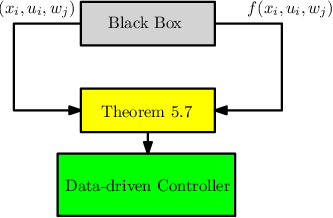
Next lemma provides an upper bound for Lipschitz constant $\mathrm{L}_{x,u}$ , which is required in Theorem 5.4, in the case that the system is affected by an additive noise.

Lemma 2

Consider a nonlinear dt-SCS as in Definition 4 which is affected by an additive noise as the following:

\displaystyle x(t+1)=f_{a}(x(t),u(t))+w(t),

(57)

and a bounded state set $X$ and input set $U$ such that $\|x\|\leq\mathcal{L}_{x}$ for all $x\in X$ , and $\|u\|\leq\mathcal{L}_{u}$ for all $u\in U$ . Without loss of generality, we assume that the mean of the noise is zero. Let $\|f_{a}(x,u)\|\leq L_{1}\|x\|+L_{2}\|u\|+L_{3}$ , $||\mathbf{J}_{x}||\leq\hat{L}_{x}$ , and $||\mathbf{J}_{u}||\leq\hat{L}_{u}$ , for some $\mathcal{L}_{x},\mathcal{L}_{u},L_{1},L_{2},L_{3},\hat{L}_{x},\hat{L}_{u}\geq 0$ , where $\mathbf{J}_{x}$ and $\mathbf{J}_{u}$ are Jacobian matrices of $f_{a}(x,u)$ with respect to $x$ and $u$ , respectively. Given a quadratic barrier function $x^{T}\mathrm{P}x$ , and a set of quadratic functions $x^{T}\mathrm{P}_{\ell}x,\;\ell\in\{1,\ldots,m\}$ , representing each of $\mathscr{P}_{\ell}(p^{\ell},x)$ with symmetric matrices $\mathrm{P}$ and $\mathrm{P}_{\ell}$ , the Lipschitz constant $\mathrm{L}_{x,u}$ can be upper-bounded by $\sqrt{\mathscr{L}_{x}^{2}+\mathscr{L}_{u}^{2}}\;$ , where

$\displaystyle\mathscr{L}_{x}$	$\displaystyle=2\mathcal{L}_{x}L_{1}\hat{L}_{x}\\|\mathrm{P}\\|+2\mathcal{L}_{u}L_{2}\hat{L}_{x}\\|\mathrm{P}\\|+2L_{3}\hat{L}_{x}\\|\mathrm{P}\\|$
	$\displaystyle\;\;\;+\mathcal{L}_{x}\\|\mathrm{P}\\|+\mathcal{L}_{x}\sum_{\ell=1}^{m}\\|\mathrm{P}_{\ell}\\|,$	(58)
$\displaystyle\mathscr{L}_{u}$	$\displaystyle=2\mathcal{L}_{x}L_{1}\hat{L}_{u}\;\\|\mathrm{P}\\|+2\mathcal{L}_{u}L_{2}\hat{L}_{u}\;\\|\mathrm{P}\\|+2L_{3}\hat{L}_{u}\;\\|\mathrm{P}\\|+\sqrt{m}.$

Proof

We first compute the Lipschitz constant regarding $\textnormal{{g}}_{5}(x,u,d)$ in (45), where

	$\displaystyle\textnormal{{g}}_{5}(x,u,d)$	$\displaystyle=~\mathds{E}\big[(f^{T}(x(t),u(t))+w^{T}(t))\mathrm{P}(f(x(t),u(t))+$
		$\displaystyle w(t))\big]+\sum_{\ell=1}^{m}(u_{\ell}-\mathscr{P}_{\ell}(p^{\ell},x))-x^{T}(t)\mathrm{P}x(t)-c.$

Considering $\mathds{E}[w(t)]=0$ , we compute the upper bounds for Lipschitz constant with respect to $x$ and $u$ separately denoted by $\mathrm{L}_{5_{x}}$ and $\mathrm{L}_{5_{u}}$ , respectively. We define $\mathbf{J}_{x}=[\frac{\partial f}{\partial x_{1}},\ldots,\frac{\partial f}{\partial x_{n}}]$ and $\mathbf{J}_{u}=[\frac{\partial f}{\partial u_{1}},\ldots,\frac{\partial f}{\partial u_{m}}]$ as Jacobian matrices with respect to $x$ and $u$ , respectively.

	$\displaystyle\mathrm{L}_{5_{x}}=$	$\displaystyle\max\limits_{x,u}\\|\frac{\partial{\textnormal{{g}}_{5}(x,u,d)}}{\partial x}\\|=\underset{x,u}{\max}\;\\|2(f(x(t),u(t))^{T}\mathrm{P}\;\mathbf{J}_{x}$
		$\displaystyle-x^{T}(t)\mathrm{P}-x^{T}(t)\sum_{\ell=1}^{m}\mathrm{P}_{\ell}\\|$
	$\displaystyle\leq$	$\displaystyle 2\mathcal{L}_{x}L_{1}\hat{L}_{x}\\|\mathrm{P}\\|+2\mathcal{L}_{u}L_{2}\hat{L}_{x}\\|\mathrm{P}\\|+2L_{3}\hat{L}_{x}\\|\mathrm{P}\\|+$
		$\displaystyle\mathcal{L}_{x}\\|\mathrm{P}\\|+\mathcal{L}_{x}\sum_{\ell=1}^{m}\\|\mathrm{P}_{\ell}\\|,$

and accordingly,

	$\displaystyle\mathrm{L}_{5_{u}}$	$\displaystyle=\max\limits_{x,u}\\|\frac{\partial{\textnormal{{g}}_{5}(x,u,d)}}{\partial u}\\|$
		$\displaystyle=\\|2(f(x(t),u(t))^{T}\mathrm{P}\mathbf{J}_{u}+\mathbf{1}_{m}\\|$
		$\displaystyle\leq 2\mathcal{L}_{x}L_{1}\hat{L}_{u}\;\\|\mathrm{P}\\|+2\mathcal{L}_{u}L_{2}\hat{L}_{u}\;\\|\mathrm{P}\\|+2L_{3}\hat{L}_{u}\;\\|\mathrm{P}\\|+\sqrt{m}.$

Now it can be deduced that

\mathrm{L}_{5}\leq\sqrt{\mathrm{L}_{5_{x}}^{2}+\mathrm{L}_{5_{u}}^{2}}.

Similar to the proof of Lemma 1, it is straightforward to compute the upper bounds of Lipschitz constants for other constraints in (45) and show that the computed upper bound is greater than all of them. We ignore this part for the sake of brevity. Then, $\mathrm{L}_{x,u}\leq\max\big(\mathrm{L}_{i},i\in\{1,2,\ldots,5+q\}\setminus\{4\}\big)=\sqrt{\mathrm{L}_{5_{x}}^{2}+\mathrm{L}_{5_{u}}^{2}}$ which is equivalent to $\sqrt{\mathscr{L}_{x}^{2}+\mathscr{L}_{u}^{2}}$ with $\mathscr{L}_{x}$ and $\mathscr{L}_{u}$ as in (2).

\textcolor

blackNote that one can use similar results as in Remark 11 to estimate the Lipschitz constant via data.

6 Data-driven Barrier Certificates for Non-convex Setting

In this section, we extend the proposed result in Section 4 to a case of having non-convex constraints. We modify the constraint (5) in Definition 3 as follows:

\displaystyle\mathds{E}\Big[\mathrm{B}(f(x,w))\mid x\Big]\leq~\kappa\;\mathrm{B}(x)+c,\quad\forall x\in X,

(59)

where $\kappa\in(0,1)$ .

According to the fundamental results in kushner1967stochastic, choosing $\kappa$ in the interval $(0,1)$ provides a better lower bound for the probability of safety satisfaction in (6), namely:

\displaystyle\mathds{P}_{w}\big(\mathcal{S}\models_{\mathcal{H}}\Psi\big)\geq 1-\rho,

with

\displaystyle\rho=\begin{cases}1-(1-\frac{1}{\lambda})(1-\frac{c}{\lambda})\qquad\qquad\qquad\qquad\text{if $\lambda\geq\frac{c}{\kappa}$}\\ \frac{1}{\lambda}(1-\kappa)^{\mathcal{H}}+\frac{c}{\kappa\lambda}\big(1-(1-\kappa)^{\mathcal{H}}\big)\;\qquad\;\;\text{if $\lambda<\frac{c}{\kappa}$},\end{cases}

(60)

where parameters $c$ , $\lambda$ , and $\mathcal{H}$ are the same as in Definition (3). Another advantage of choosing $\kappa$ in the interval $(0,1)$ is that this new formulation can be utilized in the context of compositionality and interconnected systems Zamani.2017b; SZ.19.

Replacing the last condition of RCP in (12) with the modified constraint in (59) leads to the following optimization problem which is not convex anymore:

\displaystyle\text{RP}\mathrel{\mathop{\mathchar 58\relax}}\left\{\begin{array}[]{ll}\underset{d}{\min}\quad\mathcal{K}\\ \text{s.t.}\quad\max_{z}\big(g_{z}(x,d)\big)\!\leq\!0,z\!\in\!\{1,\dots,4\},\forall x\!\in\!X,\\ \quad~~\;\;d=[\mathcal{K};\lambda;c;b_{\iota_{1},\ldots,\iota_{n}};\kappa],\\ \quad~~\;\;\mathcal{K}\in\mathbb{R},\;\lambda>1,\;c\geq 0,\;\kappa\in(0,1),\end{array}\right.

\textcolor

blackin which $g_{z}(x,d),z\in\{1,2,3\}$ , are the same as in (12), and

\displaystyle g_{4}(x,d)=\mathds{E}\Big[\mathrm{B}(f(x,w))\mid x\Big]\leq~\kappa\;\mathrm{B}(x)+c,\quad\forall x\in X.

(65)

The non-convexity comes from the multiplication of $\kappa$ and coefficients of barrier function $\mathrm{B}(b,x_{i})$ in (59). With the same reasoning in Section (3), solving the above RP is not straightforward generally. Therefore, we construct an SP by taking samples and then connect the solution of the obtained scenario programming to the safety of the stochastic system in (1). By collecting i.i.d. samples $x_{i},\;i\in\{1,\ldots,N\}$ , from an assigned probability distribution over the state set, and approximating the expectation term in (59) results in a non-convex programming as the following:

\displaystyle\text{SP\textsubscript{$\scriptscriptstyle N,\hat{N}$}}\!\mathrel{\mathop{\mathchar 58\relax}}\!\left\{\begin{array}[]{ll}\underset{d}{\min}\quad\mathcal{K}\\ \text{s.t.}\quad\;\max_{z}\,\bar{g}_{z}(x_{i},d)\!\leq\!0,\,\,\forall i\in\{1,\ldots,N\},\\ \qquad\qquad~\;\;z\!\in\!\{1,\ldots,4\},\\ \qquad~~d=[\mathcal{K};\lambda;c;b_{\iota_{1},\ldots,\iota_{n}};\kappa],\\ \qquad~~\mathcal{K}\in\mathbb{R},\;\lambda>1,\;c\geq 0,\;\kappa\in(0,1),\end{array}\right.

where $\bar{g}_{z}\mathrel{\mathop{\mathchar 58\relax}}=g_{z}$ for all $z\in\{1,2,3\}$ and

\displaystyle\bar{g}_{4}(x_{i},d)=\frac{1}{\hat{N}}\sum_{j=1}^{\hat{N}}\mathrm{B}(b,f(x_{i},w_{j}))-\;\kappa\;\mathrm{B}(b,x_{i})-c+\delta-\mathcal{K}.

(71)

Note that in this new scenario programming, we eliminated the constraint that forces a fixed probability lower bound $1-\rho$ on the safety of the stochastic system, namely, $g_{4}$ in (12). Instead, we are interested in providing the tightest possible lower bound of the safety probability according to Remark 8. The main issue underlying here is that by considering $\kappa\in(0,1)$ , the obtained scenario program is not convex anymore, and accordingly, one cannot naively utilize the results proposed in Theorems 4.3. Hence, one cannot solve the SP in (6) by simply applying bisection over $\kappa,$ while still utilizing the proposed results in the previous sections.

Now we state the main problem we aim to address in this section.

Problem 3

Consider an unknown dt-SS $\mathcal{S}$ as in Definition 1. Compute the largest lower bound $(1-\rho)\in[0,1]$ on the probability of satisfying $\Psi$ , i.e.,

\mathds{P}_{w}\big(\mathcal{S}\models_{\mathcal{H}}\Psi\big)\geq 1-\rho,

according to (60) together with a confidence $(1-\beta)\in[0,1]$ using a dataset $\mathcal{D}$ of the form (2). Moreover, establish a connection between the required size of dataset $\mathcal{D}$ , the cardinality of the set from which the parameter $\kappa$ is selected, and the desired confidence $1-\beta$ .

In the next theorem, we present our solution to Problem 3 by proposing a new confidence bound which is always valid even for the non-convex scenario program in (6).

Theorem 6.1

Consider an unknown dt-SS as in (1) together with the safety specification $\Psi$ . Let $\mathrm{M}$ be the cardinality of a finite set from \textcolorblackwhich $\kappa$ takes value in (0,1). Suppose that Assumptions 4.1-4.2 hold for the RP in (6) with function $G(\cdot)$ and $\mathrm{L}_{x}\mathrel{\mathop{\mathchar 58\relax}}=\operatorname{max}\big(\mathrm{L}_{x_{1}},\mathrm{L}_{x_{2}},\mathrm{L}_{x_{3}},\mathrm{L}_{x_{4}}\big)$ , where $\mathrm{L}_{x_{i}},i\in\{1,\ldots,4\},$ is an upper bound on the Lipschitz constant of the $i^{th}$ constraint in (6). Assume $\hat{N}$ is selected for the SP_{$\scriptscriptstyle N,\hat{N}$} similar to Theorem 3.1 in order to provide confidence $1-\beta_{s}$ . Suppose $\mathcal{K}^{\ast}(\mathcal{D})$ is the optimal value of the optimization problem in (6) using $\hat{N}$ and $N$ . Furthermore, $\epsilon=\mathrm{I}^{-1}(1-\mathrm{M}\beta;\mathcal{Q}+3,N-\mathcal{Q}-2)$ for $\beta\in[0,1]$ , where $\mathcal{Q}$ is the number of coefficients of the barrier certificate. Then the following statement holds with a confidence of at least $1-3\beta-\beta_{s}$ : if $\mathcal{K}^{\ast}(\mathcal{D})+\mathrm{L}_{x}G^{-1}(\epsilon)\leq 0$ , then

\displaystyle\mathds{P}_{w}(\mathcal{S}\models_{\mathcal{H}}\Psi)\geq 1-\rho^{\ast},

(72)

where $\rho^{\ast}$ is computed as in (60) using optimal solutions of SP_{$\scriptscriptstyle N,\hat{N}$}, namely, $c^{\ast}$ , $\lambda^{\ast}$ , and $\kappa^{\ast}$ . More importantly, with a confidence of at least $1-3\beta-\beta_{s}$ , $\mathrm{B}(b^{\ast},x)$ is a barrier certificate for $S$ , satisfying (3), (4), and (59), where $b^{\ast}$ is the optimal solution of SP_{$\scriptscriptstyle N,\hat{N}$}.

Proof

Denote the optimal values of the RP and its equivalent scenario programming before the empirical approximation of the expectation term in $g_{4}$ , namely, SP_{$\scriptscriptstyle N$}, by $\mathcal{K}^{\ast}$ and $\mathcal{K}^{\ast}_{\mathsf{m}}(\mathcal{D})$ , respectively. \textcolorblackSimilar to (30), one has

\displaystyle\mathds{P}\big(\mathcal{K}^{*}\leq\mathcal{K}^{\ast}_{\mathsf{m}}(\mathcal{D})+\mathrm{L}_{x}G^{-1}(\epsilon)\big)\geq 1-3\beta,

for any $N\geq\tilde{N}\big(\epsilon_{1},\ldots,\epsilon_{\mathrm{M}},\beta\big)$ , where

		$\displaystyle\tilde{N}\big(\epsilon_{1},\ldots,\epsilon_{\mathrm{M}},\beta\big)\mathrel{\mathop{\mathchar 58\relax}}=$
		$\displaystyle\min\Big\{N\in\mathbb{N}\mid\sum_{z=1}^{\mathrm{M}}\sum_{i=0}^{\mathrm{d}-1}\dbinom{N}{i}\epsilon_{z}^{\;i}(1-\epsilon_{z})^{N-i}\leq\beta\Big\}.$

Alternatively, one can set $\epsilon\mathrel{\mathop{\mathchar 58\relax}}=\epsilon_{1}=\epsilon_{2}=\ldots=\epsilon_{\mathrm{M}}$ in the above expression to get the inequality $\epsilon\leq\mathrm{I}^{-1}(1-\mathrm{M}\beta;\mathrm{d},N-\mathrm{d}+1)$ , where $\mathrm{M}$ is the cardinality of the set from which $\kappa$ is selected, and $\mathrm{d}$ is the number of decision variables. By choosing $\mathrm{d}\mathrel{\mathop{\mathchar 58\relax}}=\mathcal{Q}+3$ , one gets the parameters of the incomplete beta function in the theorem statement. On the other hand, due to the particular selection of $\hat{N}$ and $\beta_{s}$ similar to Theorem 3.1, it can be deduced that

\mathds{P}_{w}\Big(\hat{\mathrm{B}}(b,x\,|\,\mathcal{D})\models\text{SP\textsubscript{$\scriptscriptstyle N$}}\Big)\geq 1-\beta_{s},

where $\hat{\mathrm{B}}(b,x\,|\,\mathcal{D})$ is the barrier function whose coefficients are the optimal solution of SP_{$\scriptscriptstyle N$}. Therefore, we have

\mathds{P}\left(\mathcal{K}^{\ast}_{\mathsf{m}}(\mathcal{D})\leq\mathcal{K}^{\ast}(\mathcal{D})\right)\geq 1-\beta_{s}.

(73)

By defining events $\mathcal{A}\mathrel{\mathop{\mathchar 58\relax}}=\{\mathcal{D}\,|\,\mathcal{K}^{*}\!\leq\mathcal{K}^{\ast}_{\mathsf{m}}(\mathcal{D})+\mathrm{L}_{x}G^{-1}(\epsilon)\}$ , $\mathcal{B}\mathrel{\mathop{\mathchar 58\relax}}=\{\mathcal{D}\,|\,\mathcal{K}^{\ast}_{\mathsf{m}}(\mathcal{D})\leq\mathcal{K}^{\ast}(\mathcal{D})\}$ , and $\mathcal{C}\mathrel{\mathop{\mathchar 58\relax}}=\{\mathcal{D}\,|\,\mathcal{K}^{\ast}(\mathcal{D})+\mathrm{L}_{x}G^{-1}(\epsilon)\leq 0\}$ , where $\mathds{P}(\mathcal{A})\geq 1-3\beta$ and $\mathds{P}(\mathcal{B})\geq 1-\beta_{s}$ , it is easy to conclude using the same reasoning as in the second part of proof of Theorem (4.3) that

\displaystyle\mathds{P}(\mathcal{K}\leq 0)\geq 1-3\beta-\beta_{s},

which ensures safety of the stochastic system with a lower bound $1-\rho$ and a confidence of at least $1-3\beta-\beta_{s}$ .

7 Numerical Examples

\textcolor

blackThe simulations of this section are performed on an iMac 3.5 GHz Quad-Core Intel Core i7. The optimizations are solved by CVX Toolbox cvx with Mosek andersen2000mosek as the solver.

7.1 Temperature verification for three rooms

Consider a temperature regulation problem for three rooms characterized by the following discrete-time stochastic system:

$\displaystyle\mathrm{T}_{1}(t+1)=$	$\displaystyle\big(1-\tau_{s}(\alpha+\alpha_{e})\big)\mathrm{T}_{1}(t)+\tau_{s}\alpha\mathrm{T}_{2}(t)+$
	$\displaystyle\tau_{s}\alpha_{e}T_{e}+w_{1}(t)$
$\displaystyle\mathrm{T}_{2}(t+1)=$	$\displaystyle\big(1-\tau_{s}(2\alpha+\alpha_{e})\big)\mathrm{T}_{2}(t)+\tau_{s}\alpha(\mathrm{T}_{1}(t)+\mathrm{T}_{3}(t))+$
	$\displaystyle\tau_{s}\alpha_{e}T_{e}+w_{2}(t)$
$\displaystyle\mathrm{T}_{3}(t+1)=$	$\displaystyle\big(1-\tau_{s}(\alpha+\alpha_{e})\big)\mathrm{T}_{3}(t)+\tau_{s}\alpha\mathrm{T}_{2}(t)+$
	$\displaystyle\tau_{s}\alpha_{e}T_{e}+w_{3}(t),$	(74)

where $\mathrm{T}_{1}(t)$ , $\mathrm{T}_{2}(t)$ , and $\mathrm{T}_{3}(t)$ are temperatures of three rooms, respectively. Terms $w_{1}(t)$ , $w_{2}(t)$ , and $w_{3}(t)$ are additive zero-mean Gaussian noises with standard deviations of $0.01$ , which model the environmental uncertainties. Parameter $T_{e}=10\degree C$ is the ambient temperature. Constants $\alpha_{e}=8\times 10^{-3}$ and $\alpha=6.2\times 10^{-3}$ are heat exchange coefficients between rooms and the ambient, and individual rooms, respectively. The model for each room is adapted from girard2016safety discretized by $\tau_{s}=5$ minutes. Let us consider the regions of interest for each room as $X_{in}=[17\degree C,18\degree C]$ , $X_{u}=[29\degree C,30\degree C]$ , and $X=[17\degree C,30\degree C]$ . We assume the model of the system and the distribution of the noise are unknown. The main goal is to verify whether the temperature of each room remains in the comfort zone $[17,29]$ for the time horizon $\mathcal{H}=3$ which is equivalent to $15$ minutes, with a priori confidence of $99\%$ .

Let us consider a barrier certificate with degree $k=2$ in the polynomial form as $[T1;T2;T3]^{T}\mathrm{P}[T1;T2;T3]=b_{0}T_{1}^{2}+b_{1}T_{2}^{2}+b_{2}T_{3}^{2}+b_{3}T_{1}T_{2}+b_{4}T_{1}T_{3}+b_{5}T_{2}T_{3}+b_{6}T_{1}+b_{7}T_{2}+b_{8}T_{3}+b_{9}$ , where

\displaystyle\mathrm{P}=\begin{bmatrix}b_{0}&\frac{b_{3}}{2}&\frac{b_{4}}{2}&\frac{b_{6}}{2}\\ \frac{b_{3}}{2}&b_{1}&\frac{b_{5}}{2}&\frac{b_{7}}{2}\\ \frac{b_{4}}{2}&\frac{b_{5}}{2}&b_{2}&\frac{b_{8}}{2}\\ \frac{b_{6}}{2}&\frac{b_{7}}{2}&\frac{b_{8}}{2}&b_{9}\end{bmatrix}.

(75)

According to Algorithm 1, we first choose the desired confidence parameters $\beta$ and $\beta_{s}$ as $\frac{0.005}{3}$ and $0.005$ , respectively. The value of empirical approximation error is selected as $\delta=0.05$ . We choose $\rho=0.2$ . \textcolorblackThe Lipschitz constant is computed as $1.5$ according to Remark 11. By enforcing $\hat{M}=0.005$ , the required number of samples for the approximation of the expected value in (3) is $\hat{N}=400$ . Now, we solve the scenario problem SCP_{$\scriptscriptstyle N,\hat{N}$} with the number of samples $N=6\times 10^{6}$ and the computed $\hat{N}=400$ , which gives us the optimal objective value $\mathcal{K}^{*}(\mathcal{D})=-0.46$ . The computation time is about $5$ minutes. For $N=6\times 10^{6}$ and $\beta=\frac{0.005}{3}$ , $\epsilon$ is computed as $4.36\times 10^{-6}$ . Function $G^{-1}(\epsilon)$ is also computed as $16.09\epsilon^{\frac{1}{3}}$ according to Corollary 1.

\textcolor

blackSince $\mathcal{K}^{*}(\mathcal{D})+\mathrm{L}_{x}G^{-1}(\epsilon)=-0.066\leq 0$ , according to Theorem 4.3, one can conclude:

\displaystyle\mathds{P}_{w}(\mathcal{S}\models_{3}\Psi)\geq 1-\rho=0.80,

with a confidence of at least $1-3\beta-\beta_{s}=0.99$ . The barrier certificate constructed from solving SCP_{$\scriptscriptstyle N,\hat{N}$} is as follows:

$\displaystyle\hat{\mathrm{B}}(b,T_{1},T_{2},T_{3}\mid$	$\displaystyle\mathcal{D})=0.112T_{1}^{2}+0.112T_{2}^{2}+0.112T_{3}^{2}$
	$\displaystyle-0.004T_{1}T_{2}-0.005T_{1}T_{3}-0.002T_{2}T_{3}$
	$\displaystyle-3.761T_{1}-3.815T_{2}-3.803T_{3}+99.93.$	(76)

\textcolor

blackThe computed optimal values for $c$ and $\lambda$ are $0.627$ and $14.872$ , respectively. The scatter plot of the obtained barrier certificate is illustrated in Fig. 4. As can be seen in this figure, the barrier certificate has less values in the initial set while it has larger values in the unsafe region.

\textcolor

black We remark that the conservatism of our approach is originating from two sources. (a) The first one is that we are using barrier certificates for computing the lower bound. A barrier certificate with a fixed template (polynomial of a certain degree) gives a lower bound that could have a gap with the best lower bound on the safety probability. (b) Our sampling approach requires making the optimization more conservative to account for going from robust programs over continuous (uncountable) domains to a scenario program with finite number of samples. If one assumes that the model is known in this case study, the synthesized barrier certificate has the parameters $c=0.9767$ and $\lambda=31.51$ . This gives the lower bound $0.875$ on the safety probability. Therefore, our approach provides a more conservative lower bound $0.80$ since it assumes no knowledge of the model.

7.2 Lane keeping system

Lane keeping assist system is a future development of the modern lane departure warning system embedded in the current vehicles. This system usually assists the driver through electronic assistance with the steering force. The characteristics of this support depends on the distance of the vehicle from the edge of the lane among other factors such as uncertaintiesAnu:2013. One of the key challenges in such assisting systems is verifying the obtained performance which can be defined as a safety problem.

In this subsection, it is supposed that the model of the vehicle and the distribution of noise are unknown, and one only has access to a finite number of samples. This unknown system is characterized by a simplified kinematic single-track model of BMW320i which is adapted from althoff2017commonroad by discretization of the model and adding noise to imitate the uncertainties.

The nonlinear stochastic difference equation is as follows:

	$\displaystyle x(t+1)=x(t)+\tau_{s}v\;\cos(\psi(t)+\mathrm{b})+w_{1}(t)$
$\displaystyle\mathcal{S}\mathrel{\mathop{\mathchar 58\relax}}\;$	$\displaystyle y(t+1)=y(t)+\tau_{s}v\;\sin(\psi(t)+\mathrm{b})+w_{2}(t)$
	$\displaystyle\psi(t+1)=\psi(t)+\frac{\tau_{s}v}{l_{r}}\sin(\mathrm{b})+w_{3}(t),$	(77)

where $\mathrm{b}=\frac{l_{r}}{l_{r}+l_{f}}\tan^{-1}(\delta_{f})$ with $\delta_{f}=5$ degrees as the steering angle. Parameters $l_{r}=1.384$ and $l_{f}=1.384$ are the distances between the center of gravity of the vehicle to the rear and front axles, respectively. Variables $x$ , $y$ , and $\psi$ denote horizontal movement, vertical movement, and the heading angle, respectively. This system is considered to be affected by zero-mean additive noises $w_{1}$ , $w_{2}$ , and $w_{3}$ which are related to uncertainties of position $x$ , position $y$ , and the heading angle $\psi$ with standard deviation of $0.01$ , $0.01$ , and $0.001$ respectively. Other parameters are the sampling time $(\tau_{s}=0.1s)$ , and the velocity $(v=5m/s)$ .

The state set is considered as $X=[1,10]\times[-7,7]\times[-0.05,0.05]$ . The regions of interest are $X_{in}=[1,2]\times[-0.5,0.5]\times[-0.005,0.005]$ , $X_{u_{1}}=[1,10]\times[-7,-6]\times[-0.05,0.05]$ , and $X_{u_{2}}=[1,10]\times[6,7]\times[-0.05,0.05]$ . Now, the goal is to verify if the vehicle does not enter the unsafe regions of the lane for the time horizon of $\mathcal{H}=3$ or equivalently $0.3\;s$ with a desired confidence of $90\%$ .

We consider a barrier certificate of degree $k=2$ in the polynomial form as $[x;y;\psi]^{T}\mathrm{P}[x;y;\psi]=b_{0}x^{2}+b_{1}y^{2}+b_{2}\psi^{2}+b_{3}xy+b_{4}x\psi+b_{5}y\psi+b_{6}x+b_{7}y+b_{8}\psi+b_{9}$ , where the matrix $\mathrm{P}$ is as in (75).

\textcolor

blackWe follow Algorithm 1 to find the barrier certificate and providing a probabilistic guarantee on the safety of stochastic system. First, the desired confidence parameters $\beta$ and $\beta_{s}$ are chosen as $\frac{.095}{3}$ and $0.005$ , respectively. We also select the empirical approximation error $\delta=0.02$ . The desired lower bound of safety probability is selected as $1-\rho=0.80$ . The Lipschitz constant is computed as $\mathrm{L}_{x}=10$ according to Remark 11. By enforcing $\hat{M}=0.006$ , the required number of samples for the approximation of the expected value in (3) is $\hat{N}=3000$ . Now, we solve the scenario problem SCP_{$\scriptscriptstyle N,\hat{N}$} with an arbitrary sample number $N=6\times 10^{6}$ and $\hat{N}$ which gives us the optimal value $\mathcal{K}^{*}(\mathcal{D})=-0.4518$ . The computation time is about $5$ minutes. For those values of samples $N$ and $\beta$ , $\epsilon$ is computed as $3.41\times 10^{-6}$ . Using Corollary 1, $G^{-1}(\epsilon)$ is computed as $2.92\epsilon^{\frac{1}{3}}$ .

\textcolor

blackSince $\mathcal{K}^{*}(\mathcal{D})+2.92\;\mathrm{L}_{x}\epsilon^{\frac{1}{3}}=-0.01\leq 0$ , according to Theorem 4.3, one can deduce that

\displaystyle\mathds{P}_{w}(\mathcal{S}\models_{3}\Psi)\geq 1-\rho=0.80,

\textcolor

blackwith a confidence of at least $1-3\beta-\beta_{s}=90\%$ . The barrier certificate constructed from solving SCP_{$\scriptscriptstyle N,\hat{N}$} is represented as:

	$\displaystyle\hat{\mathrm{B}}(b,x,y,\psi\mid\mathcal{D})=$	$\displaystyle 0.39y^{2}+0.15\psi^{2}+0.009x\psi$
		$\displaystyle-0.007y\psi-0.015\psi+0.452.$		(78)

\textcolor

blackThe optimal values of $c$ and $\lambda$ are $0.57$ and $14.04$ , respectively. The exact value of the coefficients are reported in the appendix.

The surface plot of the barrier certificate $\mathrm{B}(x,y,\psi)=\hat{\mathrm{B}}(b,x,y,\psi\mid\mathcal{D})$ with respect to $x$ and $y$ for a fixed value of $\psi=0$ is depicted in Fig. 5. The blue transparent planes separate unsafe region on $y$ , while the lower and upper red transparent planes demonstrate the thresholds in constraints (3) and (4), respectively. Satisfaction of the first and second condition of barrier certificate in Definition 3 can be observed in Fig. 5. The satisfaction of the third condition is illustrated in Fig. 6.

7.3 Synthesizing a temperature controller

Consider a temperature regulation problem for a room using a heater characterized by

	$\displaystyle\textcolor{black}{\mathcal{S}}\mathrel{\mathop{\mathchar 58\relax}}\;\mathrm{T}(t+1)=$	$\displaystyle\mathrm{T}(t)+\tau_{s}\big(\alpha_{e}(T_{e}-\mathrm{T}(t))+$
		$\displaystyle\alpha_{h}(T_{h}-\mathrm{T})u(t)\big)+w(t),$		(79)

where $w(t)$ is a zero-mean Gaussian noise with standard deviation of $0.05$ . Parameters are $T_{e}=15$ , $T_{h}=45$ , $\alpha_{e}=8\times 10^{-3}$ , $\alpha_{h}=3.6\times 10^{-3}$ , and $\tau_{s}=5$ . Regions of interest are defined as $X_{in}=[22\degree C,23\degree C]$ , $X_{u_{1}}=[27\degree C,28\degree C]$ , $X_{u_{2}}=[16.5\degree C,17.5\degree C]$ , and $X=[16.5\degree C,28\degree C]$ . The input region is $[0,1]$ . We assume that the model of the system and the distribution of the noise are unknown. The main goal is to design a controller that forces the temperature to remain in the comfort zone $[17.5,27]$ for the time horizon $\mathcal{H}=60$ , which is equivalent to $300$ minutes, with a priori confidence of $95\%$ .

Let us fix a control barrier certificate with degree $k=4$ in the polynomial form as $T^{T}\mathrm{P}T=b_{0}T^{4}+b_{1}T^{3}+b_{2}T^{2}+b_{3}T+b_{4}$ with $b_{0},b_{1},b_{2},b_{3},b_{4}\in\mathbb{R}$ . The structure of the controller is considered to be a polynomial of degree $k^{\prime}=4$ as $u(p^{1},T)=T^{T}\mathrm{P}_{u}T=p_{0}T^{4}+p_{1}T^{3}+p_{2}T^{2}+p_{3}T+p_{4}$ . Matrices $\mathrm{P}$ and $\mathrm{P}_{u}$ can be represented as:

\displaystyle\mathrm{P}=\begin{bmatrix}b_{0}&\frac{b_{1}}{2}&\frac{b_{2}}{3}\\ \frac{b_{1}}{2}&\frac{b_{2}}{3}&\frac{b_{3}}{2}\\ \frac{b_{2}}{3}&\frac{b_{3}}{2}&b_{4}\end{bmatrix},\mathrm{P}_{u}=\begin{bmatrix}p_{0}&\frac{p_{1}}{2}&\frac{p_{2}}{3}\\ \frac{p_{1}}{2}&\frac{p_{2}}{3}&\frac{p_{3}}{2}\\ \frac{p_{2}}{3}&\frac{p_{3}}{2}&p_{4}\end{bmatrix}.

(80)

According to Algorithm 2, we first choose the desired confidences $\beta$ and $\beta_{s}$ as $\frac{0.005}{3}$ and $0.045$ respectively. We also select the approximation error $\delta=2$ . \textcolorblackThe Lipschitz constant $\mathrm{L}_{x,u}$ is computed as $12$ according to Remark 11. By considering $\hat{M}=1.5\times 10^{5}$ , the required number of samples for the approximation of the expected value in (3) is $\hat{N}=833330$ . Now, we solve the scenario problem SCP_{$\scriptscriptstyle N,\hat{N}$} with the selected number of samples $N=1.5\times 10^{6}$ and $\hat{N}$ which gives us the optimal value $\mathcal{K}^{*}(\mathcal{D})=-0.41$ . The computation time is about $2$ minutes. For $N=1.5\times 10^{6}$ and $\beta=\frac{0.005}{3}$ , value of $\epsilon$ is computed as $1.7424\times 10^{-5}$ . Using Corollary 3, $G^{-1}(\epsilon)$ is computed as $4.91\epsilon^{\frac{1}{2}}$ .

\textcolor

blackSince $\mathcal{K}^{*}(\mathcal{D})+\mathrm{L}_{x,u}G^{-1}(\epsilon)=-0.164\leq 0$ , one has

\displaystyle\mathds{P}_{w}^{\mathrm{p}}(\mathcal{S}\models_{60}\Psi)\geq 1-\rho=0.80,

with a confidence of at least $1-3\beta-\beta_{s}=95\%$ . The computed values for $\lambda$ and $c$ are $4817$ and $16.04$ , respectively. The control barrier certificate constructed from solving SCP_{$\scriptscriptstyle N,\hat{N}$} is:

	$\displaystyle\hat{\mathrm{B}}(b,T\mid\mathcal{D})=$	$\displaystyle\;11.89\;T^{4}-1.07\times 10^{3}\;T^{3}+3.61\times 10^{4}\;T^{2}$
		$\displaystyle-5.42\times 10^{5}+3.05\times 10^{6}.$

The obtained controller is:

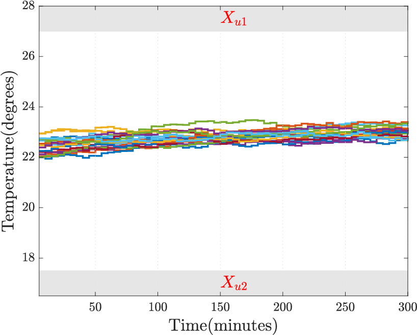
\displaystyle\mathscr{P}_{1}(p^{1},T\mid\mathcal{D})=

\displaystyle\;1.45\times 10^{-5}T^{3}+0.012T^{2}+0.355.

The temperature trajectories for $15$ different realizations of noise from three different initial temperature in the range $[22\degree,23\degree]$ is illustrated in Fig. 7. As can be seen, the temperature in the collected trajectories do not enter the unsafe set, which is in gray color. We also ran the system to get $10^{4}$ trajectories, all of them remain safe. This confirms the theoretical lower bound computed by our approach.

The conservativeness of our approach in terms of the safety bound $(1-\rho)$ and the number of samples is shown in Table 1. The values are reported for increasing number of samples and two safety thresholds with $\rho\in\{0.1,0.2\}$ . As can be seen from the table, increasing the number of samples makes $\epsilon$ smaller and reduces the term $\mathrm{L}_{x,u}G^{-1}(\epsilon)$ used in (55). In contrast, the values of $\mathcal{K}^{*}(\mathcal{D})$ become larger. This creates a tradeoff between the two terms in (55). Note that the condition of having a negative value for $\mathrm{L}_{x,u}G^{-1}(\epsilon)+\mathcal{K}^{*}(\mathcal{D})$ , thus guaranteeing safety with probability $(1-\rho)$ , is only satisfied in the last two row of the table for $\rho=0.2$ (indicated in blue color). Also, notice that the satisfaction of (55) for a higher desired safety probability requires larger number of samples.

Table 1: Conservativeness of the proposed approach

Number of samples	Computed $\epsilon$	$\mathrm{L}_{x,u}G^{-1}(\epsilon)$	$\mathcal{K}_{\rho=0.2}^{*}(\mathcal{D})$	$\mathcal{K}_{\rho=0.1}^{*}(\mathcal{D})$	$\mathcal{K}_{\rho=0.2}^{*}(\mathcal{D})+\mathrm{L}_{x,u}G^{-1}(\epsilon)$	$\mathcal{K}_{\rho=0.1}^{*}(\mathcal{D})+\mathrm{L}_{x,u}G^{-1}(\epsilon)$
$10^{3}$	$0.026$	$9.5$	$-0.48$	$-0.45$	\textcolorblack $9.02$	\textcolorblack $9.05$
$10^{4}$	$0.003$	$3$	$-0.42$	$0.09$	\textcolorblack $2.58$	\textcolorblack $3.09$
$10^{5}$	$2.61\times 10^{-4}$	$0.952$	$-0.43$	$1.37$	\textcolorblack $0.522$	\textcolorblack $2.32$
$1.5\times 10^{6}$	$1.74\times 10^{-5}$	$0.246$	$-0.41$	$2.08$	\textcolorblue $-0.164$	\textcolorblack $2.33$
$3\times 10^{6}$	$8.71\times 10^{-6}$	$0.174$	$-0.35$	$2.09$	\textcolorblue $-0.176$	\textcolorblack $2.26$

8 Conclusion

We proposed a formal verification and synthesis procedure for discrete-time continuous-space stochastic systems with unknown dynamics against safety specifications. Our approach is based on the notion of barrier certificate and uses sampled trajectories of the unknown system. We first casted the computation of the barrier certificate as a robust convex program (RCP) and approximated its solution with a scenario convex program (SCP) by replacing the unknown dynamics with the sampled trajectories. We then established that the optimal solution of the SCP gives a feasible solution for the RCP with a given confidence, and formulated a lower bound on the required number of samples. Our approach provided a lower bound on the safety probability of the stochastic unknown system when the number of sampled data is larger than a specific lower bound that depends on the desired confidence. We extended the results to a class of non-convex barrier-based safety problems and showed the applicability of our proposed approach using three case studies.

References

[1] Alessandro Abate, Daniele Ahmed, Mirco Giacobbe, and Andrea Peruffo. Formal synthesis of lyapunov neural networks. IEEE Control Systems Letters, 5(3):773–778, 2020.
[2] Matthias Althoff, Markus Koschi, and Stefanie Manzinger. Commonroad: Composable benchmarks for motion planning on roads. In 2017 IEEE Intelligent Vehicles Symposium (IV), pages 719–726. IEEE, 2017.
[3] Erling D Andersen and Knud D Andersen. The mosek interior point optimizer for linear programming: an implementation of the homogeneous algorithm. In High performance optimization, pages 197–232. Springer, 2000.
[4] Christel Baier and Joost-Pieter Katoen. Principles of model checking. MIT press, 2008.
[5] Calin Belta, Boyan Yordanov, and Ebru Aydin Gol. Formal methods for discrete-time dynamical systems, volume 15. Springer, 2017.
[6] Julian Berberich, Johannes Köhler, Matthias A Muller, and Frank Allgower. Data-driven model predictive control with stability and robustness guarantees. IEEE Transactions on Automatic Control, 2020.
[7] Urs Borrmann, Li Wang, Aaron D Ames, and Magnus Egerstedt. Control barrier certificates for safe swarm behavior. IFAC-PapersOnLine, 48(27):68–73, 2015.
[8] Giuseppe C Calafiore and Marco C Campi. The scenario approach to robust control design. IEEE Transactions on automatic control, 51(5):742–753, 2006.
[9] Andrew Clark. Control barrier functions for stochastic systems. Automatica, 130:109688, 2021.
[10] Jeremy Coulson, John Lygeros, and Florian Dörfler. Distributionally robust chance constrained data-enabled predictive control. arXiv:2006.01702, 2020.
[11] Charles Dawson, Zengyi Qin, Sicun Gao, and Chuchu Fan. Safe nonlinear control using robust neural lyapunov-barrier functions. In Conference on Robot Learning, pages 1724–1735. PMLR, 2022.
[12] Verband der Automobilindustrie. Lane keeping assist systems. https://www.vda.de/en/topics/safety-and-standards/lkas/lane-keeping-assist-systems.html, 2020.
[13] Peyman Mohajerin Esfahani, Tobias Sutter, and John Lygeros. Performance bounds for the scenario approach and an extension to a class of non-convex programs. IEEE Transactions on Automatic Control, 60(1):46–58, 2014.
[14] Antoine Girard. Reachability of uncertain linear systems using zonotopes. In International Workshop on Hybrid Systems: Computation and Control, pages 291–305. Springer, 2005.
[15] Antoine Girard, Gregor Gössler, and Sebti Mouelhi. Safety controller synthesis for incrementally stable switched systems using multiscale symbolic models. IEEE Transactions on Automatic Control, vol. 61, no. 6, pp. 1537–1549, 2016.
[16] Michael Grant and Stephen Boyd. CVX: Matlab software for disciplined convex programming, version 2.1. http://cvxr.com/cvx, March 2014.
[17] Shuo Han, Ufuk Topcu, and George J Pappas. A sublinear algorithm for barrier-certificate-based data-driven model validation of dynamical systems. In 54th IEEE conference on decision and control (CDC), pages 2049–2054, 2015.
[18] MA Hernández. Chebyshev’s approximation algorithms and applications. Computers & Mathematics with Applications, 41(3-4):433–445, 2001.
[19] Pushpak Jagtap, George J Pappas, and Majid Zamani. Control barrier functions for unknown nonlinear systems using Gaussian processes. arXiv:2010.05818, 2020.
[20] Pushpak Jagtap, Sadegh Soudjani, and Majid Zamani. Formal synthesis of stochastic systems via control barrier certificates. IEEE Transactions on Automatic Control, 66(7):3097–3110, 2020.
[21] Takafumi Kanamori and Akiko Takeda. Worst-case violation of sampled convex programs for optimization with uncertainty. Journal of Optimization Theory and Applications, 152(1):171–197, 2012.
[22] Joris Kenanian, Ayca Balkan, Raphael M Jungers, and Paulo Tabuada. Data driven stability analysis of black-box switched linear systems. Automatica, 109:108533, 2019.
[23] Yonit Kesten, Amir Pnueli, and Lion Raviv. Algorithmic verification of linear temporal logic specifications. In International Colloquium on Automata, Languages, and Programming, pages 1–16. Springer, 1998.
[24] Harold J Kushner. Stochastic stability and control. Technical report, Brown Univ Providence RI, 1967.
[25] M. Lahijanian, S. B. Andersson, and C. Belta. Formal verification and synthesis for discrete-time stochastic systems. IEEE Transactions on Automatic Control, 60(8):2031–2045, Aug 2015.
[26] Rupak Majumdar, Kaushik Mallik, and Sadegh Soudjani. Symbolic controller synthesis for Büchi specifications on stochastic systems. In Proceedings of the 23rd International Conference on Hybrid Systems: Computation and Control, pages 1–11, 2020.
[27] Vishnu Murali, Ashutosh Trivedi, and Majid Zamani. A scenario approach for synthesizing k-inductive barrier certificates. IEEE Control Systems Letters, 6:3247–3252, 2022.
[28] Ameneh Nejati, Abolfazl Lavaei, Pushpak Jagtap, Sadegh Soudjani, and Majid Zamani. Formal verification of unknown discrete- and continuous-time systems:a data-driven approach. Under review, 2021.
[29] Luyao Niu, Hongchao Zhang, and Andrew Clark. Safety-critical control synthesis for unknown sampled-data systems via control barrier functions. In 2021 60th IEEE Conference on Decision and Control (CDC), pages 6806–6813. IEEE, 2021.
[30] Swantje Plambeck, Görschwin Fey, and Schyga. Decision tree models of continuous systems. In 27th International Conference on Emerging Technologies and Factory Automation (ETFA). IEEE, 2022.
[31] Stephen Prajna and Ali Jadbabaie. Safety verification of hybrid systems using barrier certificates. In International Workshop on Hybrid Systems: Computation and Control, pages 477–492. Springer, 2004.
[32] Stephen Prajna, Ali Jadbabaie, and George J Pappas. A framework for worst-case and stochastic safety verification using barrier certificates. IEEE Transactions on Automatic Control, 52(8):1415–1428, 2007.
[33] Alexander Robey, Haimin Hu, Lars Lindemann, Hanwen Zhang, Dimos V Dimarogonas, Stephen Tu, and Nikolai Matni. Learning control barrier functions from expert demonstrations. arXiv:2004.03315, 2020.
[34] Alexander Robey, Lars Lindemann, Stephen Tu, and Nikolai Matni. Learning robust hybrid control barrier functions for uncertain systems. IFAC-PapersOnLine, 54(5):1–6, 2021.
[35] Sadra Sadraddini and Calin Belta. Formal guarantees in data-driven model identification and control synthesis. In Proceedings of the 21st International Conference on Hybrid Systems: Computation and Control (part of CPS Week), pages 147–156, 2018.
[36] Ali Salamati, Sadegh Soudjani, and Majid Zamani. Data-driven verification under signal temporal logic constraints. 21st IFAC World Congress, 2020.
[37] Christoffer Sloth, George J Pappas, and Rafael Wisniewski. Compositional safety analysis using barrier certificates. In Proceedings of the 15th ACM international conference on Hybrid Systems: Computation and Control, pages 15–24, 2012.
[38] Sadegh Soudjani and Alessandro Abate. Adaptive and sequential gridding procedures for the abstraction and verification of stochastic processes. SIAM Journal on Applied Dynamical Systems, 12(2):921–956, 2013.
[39] Sadegh Soudjani, Alessandro Abate, and Rupak Majumdar. Dynamic Bayesian networks as formal abstractions of structured stochastic processes. In 26th International Conference on Concurrency Theory, pages 169–183. Schloss Dagstuhl, 2015.
[40] Sadegh Soudjani, Caspar Gevaerts, and Alessandro Abate. Faust 2: Formal abstractions of uncountable-state stochastic processes. In 21st International Conference on Tools and Algorithms for the Construction and Analysis of Systems (TACAS 2015). Newcastle University, 2015.
[41] Sadegh Soudjani and Rupak Majumdar. Concentration of measure for chance-constrained optimization. IFAC-PapersOnLine, 51(16):277–282, 2018.
[42] Mária Svoreňová, Jan Křetínský, Martin Chmelík, Krishnendu Chatterjee, Ivana Černá, and Calin Belta. Temporal logic control for stochastic linear systems using abstraction refinement of probabilistic games. Nonlinear Analysis: Hybrid Systems, 23:230 – 253, 2017.
[43] Abdalla Swikir and Majid Zamani. Compositional synthesis of symbolic models for networks of switched systems. IEEE Control Syst. Lett., 3(4):1056–1061, 2019.
[44] Paulo Tabuada. Verification and Control of Hybrid Systems: A Symbolic Approach. Springer, 2009.
[45] Paulo Tabuada and Lucas Fraile. Data-driven stabilization of SISO feedback linearizable systems. arXiv preprint arXiv:2003.14240, 2020.
[46] Li Wang, Aaron D Ames, and Magnus Egerstedt. Safety barrier certificates for collisions-free multirobot systems. IEEE Transactions on Robotics, 33(3):661–674, 2017.
[47] Zheming Wang and Raphaël M Jungers. Data-driven computation of invariant sets of discrete time-invariant black-box systems. arXiv:1907.12075, 2019.
[48] Viraj Brian Wijesuriya and Alessandro Abate. Bayes-adaptive planning for data-efficient verification of uncertain Markov decision processes. In International Conference on Quantitative Evaluation of Systems, pages 91–108. Springer, 2019.
[49] GR Wood and BP Zhang. Estimation of the lipschitz constant of a function. Journal of Global Optimization, 8(1):91–103, 1996.
[50] Zhengfeng Yang, Min Wu, and Wang Lin. An efficient framework for barrier certificate generation of uncertain nonlinear hybrid systems. Nonlinear Analysis: Hybrid Systems, 36:100837, 2020.
[51] Majid Zamani and Murat Arcak. Compositional abstraction for networks of control systems: A dissipativity approach. IEEE Trans. Control Network Syst., 5(3):1003–1015, 2018.
[52] Majid Zamani, Peyman Mohajerin Esfahani, Rupak Majumdar, Alessandro Abate, and John Lygeros. Symbolic control of stochastic systems via approximately bisimilar finite abstractions. IEEE Transactions on Automatic Control, 59(12):3135–3150, 2014.
[53] Majid Zamani, Ilya Tkachev, and Alessandro Abate. Towards scalable synthesis of stochastic control systems. Discrete Event Dynamic Systems, 27(2):341–369, 2017.
[54] Lijun Zhang, Zhikun She, Stefan Ratschan, Holger Hermanns, and Ernst Moritz Hahn. Safety verification for probabilistic hybrid systems. In International Conference on Computer Aided Verification, pages 196–211. Springer, 2010.

9 Lipschitz continuity of the max function

\textcolor

black

Lemma 3

The maximum of Lipschitz continuous functions $f_{i}\mathrel{\mathop{\mathchar 58\relax}}X\rightarrow\mathbb{R}$ , $i=1,2,\ldots,m$ , is a Lipschitz continuous function. The Lipschitz constant of the maximum is the sum of the Lipschitz constants of $f_{i}$ .

Proof

\textcolor

blackSuppose that two Lipschitz continuous functions $f_{1}$ and $f_{2}$ have Lipschitz constants $L_{1}$ and $L_{2}$ , respectively. One can rewrite $g=\max(f_{1},f_{2})$ as:

\displaystyle g=\max(f_{1},f_{2})=\frac{f_{1}+f_{2}+|f_{1}-f_{2}|}{2}.

Then, we can use triangle inequality to show that

	$\displaystyle\|g(x)-g(y)\|$	$\displaystyle\leq\frac{1}{2}[\|f_{1}(x)-f_{1}(y)\|+\|f_{2}(x)-f_{2}(y)\|+$
		$\displaystyle\big\|\|f_{1}(x)-f_{2}(x)\|-\|f_{1}(y)-f_{2}(y)\|\big\|]$
		$\displaystyle\leq\frac{1}{2}[L_{1}\\|x-y\\|+L_{2}\\|x-y\\|+\|f_{1}(x)-f_{1}(y)\|+$
		$\displaystyle\|f_{2}(x)-f_{2}(y)\|]\leq\frac{1}{2}[L_{1}\\|x-y\\|+L_{2}\\|x-y\\|+$
		$\displaystyle L_{1}\\|x-y\\|+L_{2}\\|x-y\\|]=(L_{1}+L_{2})\\|x-y\\|.$

Therefore, $\max(f_{1},f_{2})$ is also a Lipschitz continuous function with Lipschitz constant $L_{1}+L_{2}$ . This argument can be extended inductively to the maximum of every number of functions.

Lemma 4

\textcolor

blackFor any two analytic functions $f_{1}\mathrel{\mathop{\mathchar 58\relax}}X\rightarrow\mathbb{R}$ and $f_{2}\mathrel{\mathop{\mathchar 58\relax}}X\rightarrow\mathbb{R}$ with a compact domain $X$ , $L\mathrel{\mathop{\mathchar 58\relax}}=\max(L_{1},L_{2})$ is a Lipschitz constant of $\max(f_{1},f_{2})$ .

Proof

\textcolor

black Note that

g(x)=\max(f_{1}(x),f_{2}(x))=\begin{cases}f_{1}(x)&\text{if}\quad f_{1}(x)-f_{2}(x)\geq 0\\ f_{2}(x)&\text{if}\quad f_{1}(x)-f_{2}(x)\leq 0.\end{cases}

The function $f_{1}-f_{2}$ is also analytic, thus has a finite number of zeros in a compact domain. Let us denote the finite set of zeros as $Z$ . We first show this for one-dimensional compact domains $X\subset\mathbb{R}$ . Take two points $x,y\in X$ such that $x<y$ , and define $Z\cap[x,y]=\{z_{1},z_{2},\ldots,z_{m}\}$ such that $z_{i}<z_{i+1}$ for any $i=1,2,\ldots,m-1$ . Then we have

	$\displaystyle\|g(y)-g(x)\|=\|f_{i_{y}}(y)-f_{i_{m}}(z_{m})$	$\displaystyle+f_{i_{m}}(z_{m})-f_{i_{m-1}}(z_{m-1})+\ldots$
		$\displaystyle+f_{i_{2}}(z_{2})-f_{i_{1}}(z_{1})+f_{i_{1}}(z_{1})-f_{i_{x}}(x)\|,$

for some appropriate choices of $i_{x},i_{y},i_{1},\ldots,i_{m}$ all from the set $\{1,2\}$ . Since $g(z_{j})=f_{1}(z_{j})-f_{2}(z_{j})=0$ , we can set the index of $f$ to symbol that belongs to the set $\{1,2\}$ when the function is evaluated at any $z_{j}$ . Then, we have

		$\displaystyle\|g(y)-g(x)\|$
		$\displaystyle=\|f_{i_{y}}(y)-f_{i_{y}}(z_{m})+f_{i_{m}}(z_{m})-f_{i_{m}}(z_{m-1})+\ldots+$
		$\displaystyle f_{i_{2}}(z_{2})-f_{i_{2}}(z_{1})+f_{i_{x}}(z_{1})-f_{i_{x}}(x)\|\leq$
		$\displaystyle\|f_{i_{y}}(y)-f_{i_{y}}(z_{m})\|+\|f_{i_{m}}(z_{m})-f_{i_{m}}(z_{m-1})\|+\ldots+$
		$\displaystyle\|f_{i_{2}}(z_{2})-f_{i_{2}}(z_{1})\|+\|f_{i_{x}}(z_{1})-f_{i_{x}}(x)\|$
		$\displaystyle\leq L_{i_{y}}(y-z_{m})+L_{i_{m}}(z_{m}-z_{m-1})+\ldots+$
		$\displaystyle L_{i_{2}}(z_{2}-z_{1})+L_{i_{x}}(z_{1}-x)$
		$\displaystyle L(y-z_{m})+L(z_{m}-z_{m-1})+\ldots+L(z_{2}-z_{1})+L(z_{1}-x)$
		$\displaystyle=L(y-x),$

where $L=\max(L_{1},L_{2})=\max(L_{i_{y}},L_{i_{x}},L_{i_{1}},\ldots,L_{i_{m}})$ . This concludes the proof for one-dimensional case.

\textcolor

blackWe now prove the statement for multi-dimensional case. Take two points $x,y\in X\subset\mathbb{R}^{n}$ with $x=(x_{1},\ldots,x_{n})$ and $y=(y_{1},\ldots,y_{n})$ . The functions $f_{1},f_{2}$ have Lipschitz constants $L_{1},L_{2}$ , which means

|f_{i}(y_{1},\ldots,y_{n})-f_{i}(x_{1},\ldots,x_{n})|\leq L_{i}\|(y_{1}-x_{1},\ldots,y_{n}-x_{n})\|,\quad i\in\{1,2\}.

(81)

Define the line segment that connects these two points as $D\mathrel{\mathop{\mathchar 58\relax}}=\{\lambda y+(1-\lambda)x\,|\,\lambda\in[0,1]\}$ . Let us know restrict the domain of the function $g$ to $D$ and define:

		$\displaystyle h\mathrel{\mathop{\mathchar 58\relax}}[0,1]\rightarrow\mathbb{R},\quad h(\lambda)\mathrel{\mathop{\mathchar 58\relax}}=g(\lambda y+(1-\lambda)x)=$
		$\displaystyle\max(f_{1}(\lambda y+(1-\lambda)x),f_{2}(\lambda y+(1-\lambda)x)).$

We can now apply the first part of the proof to get:

|h(1)-h(0)|\leq L^{\prime}|1-0|,

(82)

where $L^{\prime}$ is the maximum of the Lipschitz constants of $f_{1}(\lambda y+(1-\lambda)x)$ and $f_{2}(\lambda y+(1-\lambda)x)$ with respect to $\lambda$ . To get these Lipschitz constants, we use (81):

		$\displaystyle\|f_{i}(\lambda_{1}y+(1-\lambda_{1})x)-f_{i}(\lambda_{2}y+(1-\lambda_{2})x)\|\leq$
		$\displaystyle L_{i}\\|(\lambda_{1}-\lambda_{2})(y-x)\\|=L_{i}\|\lambda_{1}-\lambda_{2}\|\,\\|y-x\\|$
		$\displaystyle=(L_{i}\\|y-x\\|)\,\|\lambda_{1}-\lambda_{2}\|$

Therefore, the Lipschitz constants of $f_{1}(\lambda y+(1-\lambda)x)$ for a given $x,y$ with respect to $\lambda$ is $L_{i}\|y-x\|$ . Replacing definitions in (82), we have

|g(y)-g(x)|\leq L^{\prime}=\max(L_{1}\|y-x\|,L_{2}\|y-x\|)=\|y-x\|\max(L_{1},L_{2}).

This completes the proof.

\textcolor

black

10 Proof of Corollary 1

\displaystyle\mathds{P}[\mathrm{b}(x,r)]\geq G(r),\qquad\forall x\in X.

Since we assume that samples are collected uniformly, $\mathds{P}[\mathrm{b}(x,r)]$ for every small ball centered at every $x\in X$ with radius $r=\epsilon$ can be computed by dividing the volume of this ball by the whole state set volume. Given that one needs to find the maximum ball that is valid for $\forall x\in X$ , and some points $x$ lie on the border of the hyper-rectangular state set, the maximum ball is a semi-hypersphere in general, whose volume can be computed as $\dfrac{1}{2^{n}}\frac{\pi^{\frac{n}{2}}}{\Gamma(\frac{n}{2}+1)}\epsilon^{n}$ with the Gamma function defined as $\Gamma(k)=1\times 2\times 3\ldots\times(k-1)$ and $\Gamma(k+\frac{1}{2})=\frac{1}{2}\times\frac{3}{2}\times\ldots(k-\frac{3}{2})(k-\frac{1}{2})\pi^{\frac{1}{2}}$ for all positive integers. Dividing this value by the whole state set volume, which is $\prod_{i=1}^{n}\eta_{x}(i)$ for $\eta_{x}(i)$ as the length of the edges in each direction, gives us $G(\epsilon)$ .

\textcolor

black

11 Proof of Corollary 2

The proof is similar to the proof of Corollary 1 in 10. Here, the centered ball with the maximum volume is the intersection of the whole state set sphere and the small ball $r=\epsilon$ centered at any point on the border of the state set sphere. The volume of this intersection, which is the volume of two separate caps, can be computed as:

\displaystyle V_{n}^{cap}(\tilde{r},\rm c_{1})+V_{n}^{cap}(\epsilon,\rm c_{2}),

where

\displaystyle V_{n}^{cap}(\tilde{r},\rm c_{1})=\frac{1}{2}\frac{\pi^{\frac{n}{2}}}{\Gamma(\frac{n}{2}+1)}\tilde{r}^{n}\mathrm{I}(1-\frac{\rm c_{1}^{2}}{\tilde{r}^{2}};\frac{n+1}{2},\frac{1}{2}),

and

\displaystyle V_{n}^{cap}(\epsilon,\rm c_{2})=\frac{1}{2}\frac{\pi^{\frac{n}{2}}}{\Gamma(\frac{n}{2}+1)}\epsilon^{n}\mathrm{I}(1-\frac{\rm c_{2}^{2}}{\epsilon^{2}};\frac{n+1}{2},\frac{1}{2}),

for $\rm c_{1}=\frac{2\tilde{r}^{2}-\epsilon^{2}}{2\tilde{r}}$ , and $\rm c_{2}=\frac{\epsilon^{2}}{2\tilde{r}}$ . By dividing the intersection volume by the volume of the whole hypersphere state set, which is

\displaystyle V_{n}(\tilde{r})=\frac{\pi^{\frac{n}{2}}}{\Gamma(\frac{n}{2}+1)}\tilde{r}^{n},

one can compute $G(\epsilon)$ as in Corollary 2.

\textcolor

black

12 Coefficients of the computed barrier certificates in floating point format with 16 digits.

Temperature Verification	Lane Keeping	Synthesizing a
for 3 Rooms	System	Controller
$1.118824712343290\times 10^{-1}$	$2.200050812923097\times 10^{-4}$	$1.189325015407815\times 10$
$1.121295401333170\times 10^{-1}$	$3.901846347425760\times 10^{-1}$	$-1.070392322770013\times 10^{3}$
$1.122576531449860\times 10^{-1}$	$1.480240596483330\times 10^{-1}$	$3.612276124685787\times 10^{4}$
$-3.751401155407000\times 10^{-3}$	$-2.825312554914731\times 10^{-4}$	$-5.417521260597183\times 10^{5}$
$-4.728480781000000\times 10^{-3}$	$9.905388481691000\times 10^{-3}$	$3.046603167514221\times 10^{6}$
$-2.284303936564000\times 10^{-3}$	$-6.672383448890000\times 10^{-3}$	-
$-3.761231117922648\times 10^{0}$	$-6.918249590565419\times 10^{-4}$	-
$-3.815332731044874\times 10^{0}$	$4.678025224577894\times 10^{-4}$	-
$-3.803570830339135\times 10^{0}$	$-1.539512818952500\times 10^{-2}$	-
$9.993049903406006\times 10$	$4.518033593474370\times 10^{-1}$	-

\textcolor

blackIn the above table, the values in first two columns from top to the bottom are $\{b_{0},\ldots,b_{9}\}$ in respective case studies. The values in the the third column from top to the bottom are $\{b_{0},\ldots,b_{4}\}$ in the last case study.

	$\displaystyle L_{x_{5}}$	$\displaystyle=\underset{x}{\max}\\|2(f(x(t))^{T}\mathrm{P}\;\mathbf{J}_{x}-x^{T}(t)\mathrm{P})\\|$
		$\displaystyle\leq\underset{x}{\max}\;\;2\\|f(x(t))^{T}\\|\\|\mathrm{P}\\|\\|\mathbf{J}_{x}\\|+2\\|x^{T}(t)\\|\\|\mathrm{P}\\|$
		$\displaystyle\leq 2(L_{1}\mathcal{L}+L_{2})\\|\mathrm{P}\\|\hat{L}+2\mathcal{L}\\|\mathrm{P}\\|$
		$\displaystyle=2\\|\mathrm{P}\\|(L_{1}\mathcal{L}\hat{L}+L_{2}\hat{L}+\mathcal{L}).$

	$\displaystyle\mathrm{L}_{5_{x}}=$	$\displaystyle\max\limits_{x,u}\\|\frac{\partial{\textnormal{{g}}_{5}(x,u,d)}}{\partial x}\\|=\underset{x,u}{\max}\;\\|2(f(x(t),u(t))^{T}\mathrm{P}\;\mathbf{J}_{x}$
		$\displaystyle-x^{T}(t)\mathrm{P}-x^{T}(t)\sum_{\ell=1}^{m}\mathrm{P}_{\ell}\\|$
	$\displaystyle\leq$	$\displaystyle 2\mathcal{L}_{x}L_{1}\hat{L}_{x}\\|\mathrm{P}\\|+2\mathcal{L}_{u}L_{2}\hat{L}_{x}\\|\mathrm{P}\\|+2L_{3}\hat{L}_{x}\\|\mathrm{P}\\|+$
		$\displaystyle\mathcal{L}_{x}\\|\mathrm{P}\\|+\mathcal{L}_{x}\sum_{\ell=1}^{m}\\|\mathrm{P}_{\ell}\\|,$

	$\displaystyle\mathrm{L}_{5_{u}}$	$\displaystyle=\max\limits_{x,u}\\|\frac{\partial{\textnormal{{g}}_{5}(x,u,d)}}{\partial u}\\|$
		$\displaystyle=\\|2(f(x(t),u(t))^{T}\mathrm{P}\mathbf{J}_{u}+\mathbf{1}_{m}\\|$
		$\displaystyle\leq 2\mathcal{L}_{x}L_{1}\hat{L}_{u}\;\\|\mathrm{P}\\|+2\mathcal{L}_{u}L_{2}\hat{L}_{u}\;\\|\mathrm{P}\\|+2L_{3}\hat{L}_{u}\;\\|\mathrm{P}\\|+\sqrt{m}.$

	$\displaystyle\|g(x)-g(y)\|$	$\displaystyle\leq\frac{1}{2}[\|f_{1}(x)-f_{1}(y)\|+\|f_{2}(x)-f_{2}(y)\|+$
		$\displaystyle\big\|\|f_{1}(x)-f_{2}(x)\|-\|f_{1}(y)-f_{2}(y)\|\big\|]$
		$\displaystyle\leq\frac{1}{2}[L_{1}\\|x-y\\|+L_{2}\\|x-y\\|+\|f_{1}(x)-f_{1}(y)\|+$
		$\displaystyle\|f_{2}(x)-f_{2}(y)\|]\leq\frac{1}{2}[L_{1}\\|x-y\\|+L_{2}\\|x-y\\|+$
		$\displaystyle L_{1}\\|x-y\\|+L_{2}\\|x-y\\|]=(L_{1}+L_{2})\\|x-y\\|.$

		$\displaystyle\|g(y)-g(x)\|$
		$\displaystyle=\|f_{i_{y}}(y)-f_{i_{y}}(z_{m})+f_{i_{m}}(z_{m})-f_{i_{m}}(z_{m-1})+\ldots+$
		$\displaystyle f_{i_{2}}(z_{2})-f_{i_{2}}(z_{1})+f_{i_{x}}(z_{1})-f_{i_{x}}(x)\|\leq$
		$\displaystyle\|f_{i_{y}}(y)-f_{i_{y}}(z_{m})\|+\|f_{i_{m}}(z_{m})-f_{i_{m}}(z_{m-1})\|+\ldots+$
		$\displaystyle\|f_{i_{2}}(z_{2})-f_{i_{2}}(z_{1})\|+\|f_{i_{x}}(z_{1})-f_{i_{x}}(x)\|$
		$\displaystyle\leq L_{i_{y}}(y-z_{m})+L_{i_{m}}(z_{m}-z_{m-1})+\ldots+$
		$\displaystyle L_{i_{2}}(z_{2}-z_{1})+L_{i_{x}}(z_{1}-x)$
		$\displaystyle L(y-z_{m})+L(z_{m}-z_{m-1})+\ldots+L(z_{2}-z_{1})+L(z_{1}-x)$
		$\displaystyle=L(y-x),$