Recursive one-way Navier Stokes equations
with PSE-like cost

We begin with the compressible Navier-Stokes equations (including mass, momemntum, and energy equations), written schematically as

$$\frac{\partial q}{\partial t}=\mathcal{N}(q).$$

(2.1)

The state vector $q(x,y,z,t)\in R^{N_{q}}$ contains velocity components and two thermodynamics variales, e.g., density and pressure, and $N_{q}$ is the number of the state variables, i.e., $N_{q}=5$ for three-dimensional flows.

The Navier-Stokes operator $\mathcal{N}$ in (2.1) is nonlinear. Applying the Reynolds decomposition,

$$q(x,y,z,t)=\overline{q}(x,y,z)+q^{\prime}(x,y,z,t),$$

(2.2)

and moving terms that are linear and nonlinear in the perturbation $q^{\prime}$ to the left-hand-side and right-hand-side, respectively, results in an equation of the form

$$\frac{\partial q^{\prime}}{\partial t}+Lq^{\prime}=f,$$

(2.3)

where

$${L}(\overline{q})=\frac{\partial\mathcal{N}}{\partial q}\bigg\rvert_{\bar{q}}$$

(2.4)

is the linearized Navier-Stokes operator and $f=f(\overline{q},q^{\prime})$ contains the remaining nonlinear terms, which we view as a forcing on the linearized equations. More generally, $f$ may contain both the nonlinear terms as well as exogenous forcing applied to the flow stemming from boundary conditions, control actuation, and so on.

To enable development of a one-way equation, we separate the linear operator into two parts,

$$L=A\frac{\partial}{\partial x}+B.$$

(2.5)

Here, $x$ is the coordinate direction in which the mean flow is slowly varying, and thus the direction in which we wish to spatially integrate the equations. In (2.5), we have isolated the derivatives in the $x$ direction, and all other terms from $L$ are in the operator $B$. The linear operator ${L}$ also contains the second derivative in $x$ arising from the viscous terms in the Navier-Stokes equations. While not strictly necessary [27, 31], we neglect these terms in the present formulation for the sake of simplicity and note that extensive testing has shown them to be unimportant in a variety of flows [26]. Substituting (2.5) into (2.3), we have

$$\frac{\partial q^{\prime}}{\partial t}+{A}\frac{\partial q^{\prime}}{\partial x}+{B}q^{\prime}=f.$$

(2.6)

Discretizing (2.6) in the transverse directions, i.e., $y$ and $z$, using a collocation method such as finite differences leads to the the semi-discrete form

$$\frac{\partial\boldsymbol{q}^{\prime}}{\partial t}+\boldsymbol{A}\frac{\partial\boldsymbol{q}^{\prime}}{\partial x}+\boldsymbol{B}\boldsymbol{q}^{\prime}=\boldsymbol{f}.$$

(2.7)

Here, $\boldsymbol{q}^{\prime}\in R^{N}$ and $\boldsymbol{A},\boldsymbol{B}\in R^{N\times N}$ are the semi-discrete forms of $q^{\prime}$, $A$, and $B$, respectively, and $N=N_{q}\times N_{d}$ is the size of the discretized state, where $N_{d}$ is the total number of discretization points in the transverse directions.

Previous OWNS variants proceed by transforming the state vector $\boldsymbol{q}^{\prime}$ and its governing equation (2.6) into characteristic space, which aids in developing recursion equations that lead to efficient implementations of the one-way equations. While this is not necessary for the current formulation, we follow this precedent to enable straightforward comparisons with these earlier variants. Characteristic variables are obtained via the transformation

$$\boldsymbol{\phi}(x,t)=\boldsymbol{T}(x)\boldsymbol{q}^{\prime}(x,t),$$

(2.8)

where $\boldsymbol{T}$ is a matrix containing the eigenvectors of $\boldsymbol{A}$,

$$\boldsymbol{TAT}^{-1}=\tilde{\boldsymbol{A}},$$

(2.9)

and $\tilde{\boldsymbol{A}}$ is a diagonal matrix containing the eigenvalues. Then (2.7) can be written in terms of the characteristic variables as

$$\frac{\partial\boldsymbol{\phi}}{\partial t}+\tilde{\boldsymbol{A}}\frac{\partial\boldsymbol{\phi}}{\partial x}+\tilde{\boldsymbol{B}}\boldsymbol{\phi}=\boldsymbol{f}_{\phi},$$

(2.10)

where $\boldsymbol{f}_{\phi}=\boldsymbol{T}\boldsymbol{f}$ and $\tilde{\boldsymbol{B}}=\boldsymbol{TBT}^{-1}+\tilde{\boldsymbol{A}}\boldsymbol{T}\frac{\mathrm{d}\boldsymbol{T}^{-1}}{\mathrm{d}x}$.

Our goal is to obtain a one-way equation in the frequency (Fourier) domain. However, we begin by applying a more general Laplace transform in time, which enables a rigorous identification of rightgoing and leftgoing waves. Taking a Laplace transform of (2.10) gives

$$s\hat{\boldsymbol{\phi}}+\tilde{\boldsymbol{A}}\frac{\partial\hat{\boldsymbol{\phi}}}{\partial x}+\tilde{\boldsymbol{B}}\hat{\boldsymbol{\phi}}=\hat{\boldsymbol{f}}_{\phi},$$

(2.11)

where $\hat{\boldsymbol{\phi}}(x,s)$ is the Laplace transform of $\boldsymbol{\phi}(x,t)$, $s=\eta-i\omega$, $i$ is the imaginary unit, and $\eta$ and $\omega$ are real scalars. We will later set $\eta=0$ to revert to the Fourier domain. Solving for $x$ derivatives, (2.11) can be written as

$$\frac{\mathrm{d}\hat{\boldsymbol{\phi}}}{\mathrm{d}x}=\boldsymbol{M}(x,s)\hat{\boldsymbol{\phi}}+\hat{\boldsymbol{g}}(x,s)$$

(2.12)

with

		$\displaystyle\boldsymbol{M}=-\tilde{\boldsymbol{A}}^{-1}(s\boldsymbol{I}+\tilde{\boldsymbol{B}}),$		(2.13a)
		$\displaystyle\hat{\boldsymbol{g}}=\tilde{\boldsymbol{A}}^{-1}\hat{\boldsymbol{f}}_{\phi}.$		(2.13b)

Here, we have assumed that $\boldsymbol{A}$, and thus $\tilde{\boldsymbol{A}}$, is full rank. A simple procedure for accommodating a singular $\boldsymbol{A}$ is presented in Appendix A, and we note that handling this case is considerably more straightforward within the OWNS-R formulation than in OWNS-P [28].

The manipulations leading from (2.1) to (2.12) have produced a form more conducive to the analysis to follow but have not altered the basic character of the equations. Indeed, a global solution of the linearized equations could be obtained by discretizing (2.12) in the $x$ direction, applying boundary conditions at the begining and end of the $x$ domain, and solving the resulting linear system of equations. However, this approach is computationally costly and does not leverage the slow variation of the mean flow. Instead, the solution of (2.12) can be obtained by spatial integration. While integrating (2.12) is nominally ill-posed and numerically unstable, these issues can be overcome by removing leftgoing components of the solution that are responsible for the ill-posedness and instability.

To this end, consider the eigen-decomposition of the spatial marching operator,

$$\boldsymbol{M}=\boldsymbol{VDV}^{-1}=\boldsymbol{V}i\boldsymbol{\Lambda}\boldsymbol{V}^{-1}.$$

(2.14)

The eigenvalues and eigenvectors of $\boldsymbol{M}$ are located in the columns of $\boldsymbol{V}$ and in the diagonal matrix $\boldsymbol{\Lambda}$, respectively. Here, we have assumed that $\boldsymbol{M}$ has a full basis of eigenvectors; the defective case is discussed in detail by Towne et al. [26]. The solution of (2.12) can be written as an expansion in the eigenvectors of $\boldsymbol{M}$,

$$\hat{\boldsymbol{\phi}}(x)=\sum_{i=1}^{N}{\boldsymbol{v}_{k}(x)\psi_{k}(x)}=\boldsymbol{V\psi},$$

(2.15)

where $\boldsymbol{v}_{k}$ is the $k$-th eigenvector of $\boldsymbol{M}$, $\psi_{k}$ is the associated expansion coefficient that determines the contribution of the eigenvector to the state vector, and $\boldsymbol{\psi}\in C^{N}$ is a vector containing all of the expansion coefficients.

The solution contains contributions from both rightgoing modes and leftgoing modes. Briggs criteria [32], and its extension to non-parallel flows [33, 13, 26], provides a rigorous means to distinguish between rightgoing and leftgoing modes. Denote $\alpha_{k}(x,s)$ as the eigenvalue corresponding to the eigenvector $\boldsymbol{v}_{k}$, i.e., the $k$-th element in $\boldsymbol{\Lambda}$. Then the $k$-th mode is rightgoing at $x=x_{0}$ if

$$\lim_{\eta\to+\infty}\text{Im}[\alpha_{k}(x_{0},s)]=+\infty$$

(2.16)

and leftgoing at $x=x_{0}$ if

$$\lim_{\eta\to+\infty}\text{Im}[\alpha_{k}(x_{0},s)]=-\infty.$$

(2.17)

After the modes are classified, $\boldsymbol{V}$ and $\boldsymbol{\psi}$ can be reorganized as

$$\boldsymbol{V}=\begin{bmatrix}\boldsymbol{V}_{+}&\boldsymbol{V}_{-}\end{bmatrix},\quad\boldsymbol{\psi}=\begin{bmatrix}\boldsymbol{\psi}_{+}\\ \boldsymbol{\psi}_{-}\end{bmatrix},$$

(2.18)

where $\boldsymbol{V}_{+}$ and $\boldsymbol{V}_{-}$ contain the eigenvectors of rightgoing and leftgoing modes, respectively, and $\boldsymbol{\psi}_{+}$ and $\boldsymbol{\psi}_{-}$ contain the corresponding expansion coefficients. Using this partitioning, (2.15) can be written as

$$\hat{\boldsymbol{\phi}}(x)=\sum_{i=1}^{N_{+}}{\boldsymbol{v}_{k}(x)\psi_{k}(x)}+\sum_{i={N_{+}}+1}^{N_{+}+N_{-}}{\boldsymbol{v}_{k}(x)\psi_{k}(x)}=\boldsymbol{V}_{+}\boldsymbol{\psi}_{+}+\boldsymbol{V}_{-}\boldsymbol{\psi}_{-}.$$

(2.19)

Here, $N_{+}$ and $N_{-}$ are the number of rightgoing and leftgoing modes, respectively, and $N_{+}+N_{-}=N$.

If (2.12) is spatially integrated in the positive $x$ (rightgoing) direction, leftgoing modes that physically represent waves that decay as they travel in the negative $x$ direction will be wrongly captured as growing rightgoing modes, leading to exponential instability in the march. In order to make the problem well-posed and stabilize the march, the contribution of leftgoing modes, i.e. the second summation in (2.19), must be eliminated. In the following section, we will discuss how to eliminate the leftgoing modes, beginning with an exact formulation followed by a computationally efficient approximation.

A projection operator that exactly eliminates leftgoing modes can be written in terms of the eigenvectors of $\boldsymbol{M}$ [27, 28], i.e.,

$$\boldsymbol{P}=\boldsymbol{V}\boldsymbol{E}\boldsymbol{V}^{-1}=\begin{bmatrix}\boldsymbol{V}_{+}&\boldsymbol{V}_{-}\end{bmatrix}\begin{bmatrix}\boldsymbol{I}_{++}&\\ &\boldsymbol{0}_{--}\end{bmatrix}\begin{bmatrix}\boldsymbol{V}_{+}&\boldsymbol{V}_{-}\end{bmatrix}^{-1},$$

(2.20)

where $\boldsymbol{I}_{++}\in R^{N_{+}\times N_{+}}$ is an identity matrix and $\boldsymbol{0}_{--}\in R^{N_{-}\times N_{-}}$ is the null matrix. Applying this projection operator to the state vector $\hat{\boldsymbol{\phi}}$ gives

$$\hat{\boldsymbol{\phi}}^{\prime}\triangleq\boldsymbol{P}\hat{\boldsymbol{\phi}}=\boldsymbol{P}\boldsymbol{V}\boldsymbol{\psi}=\boldsymbol{V}_{+}\boldsymbol{\psi}_{+}=\sum_{i=1}^{N_{+}}{\boldsymbol{v}_{i}\psi_{i}}.$$

(2.21)

It is clear from (2.21) that the projection operator eliminates the leftgoing modes such that the projected state vector $\hat{\boldsymbol{\phi}}^{\prime}$ contains only rightgoing modes, as desired. Equivalently, this can be expressed as a relationship between the expansion coefficients for the projected and original states,

$$\boldsymbol{\psi}^{\prime}=\boldsymbol{E}\boldsymbol{\psi}.$$

(2.22)

Since the eigenvalues of $\boldsymbol{P}$ contained within the diagonal matrix $\boldsymbol{E}$ are one for rightgoing modes and zero for leftgoing modes, the expansion coefficients for rightgoing modes are unaltered, while the expansion coefficients for leftgoing modes have been set to zero by the projection.

In the previous OWNS-P method, this projection operator (and approximations thereof) is used to obtain a one-way evolution equation for the projected state vector $\hat{\boldsymbol{\phi}}^{\prime}$ by projecting (2.12). In the present work, we instead use it to project out the influence of the leftgoing modes at each step in the march as (2.12) is integrated. This simplifies the formulation and implementation of the method, and we will show in Section 3.2 that these two procedures are closely related. The equations can also be integrated in the opposite, upstream direction to obtain an approximation of the leftgoing modes using the projection $\boldsymbol{I}-\boldsymbol{P}$ in place of $\boldsymbol{P}$.

The projection operator (2.20) is exact, but its formation requires the eigen-decomposition of the spatial marching operator $\boldsymbol{M}$ at every $x$ station in the spatial march. While such an approach has been pursued by others [34], this is prohibitively expensive, e.g., more expensive than simply solving the global problem to begin with, except in some special cases, e.g., problems that are homogeneous in the $x$ direction or that posses a small number of relevant eigenmodes. To make the OWNS formulation useful, efficient approximations of the projection operator are needed.

An approximate projection operator was developed as part of the OWNS-P method [27, 28], as discussed in the introduction. However, the computational cost associated with building the approximate OWNS-P projection operator remains significant; it is typically around three times more costly than OWNS-O and ten to one hundred times more costly than PSE. In this paper, we develop a new approximation of the exact projection operator whose cost (per step) approaches that of PSE while retaining the accuracy of previous OWNS methods. The two formulations are compared in detail in Section 3.

Our new approximate projection operator takes the form

$$\boldsymbol{P}_{N_{\beta}}=(\boldsymbol{I}+c\boldsymbol{Z})^{-1},$$

(2.23)

where

$$\boldsymbol{Z}=\prod\limits_{j=1}^{N_{\beta}}{(\boldsymbol{M}-i\beta_{j}^{+}\boldsymbol{I})(\boldsymbol{M}-i\beta_{j}^{-}\boldsymbol{I})^{-1}}.$$

(2.24)

As in previous variant of OWNS [26, 27, 28], we have introduced a set of recursion parameters $\left\{\beta_{j}^{+},\beta_{j}^{-}:j=1,2,...,N_{\beta}\right\}$, and $c$ is an additional parameter whose effect will be elaborated later. The approximate projection operator $\boldsymbol{P}_{N_{\beta}}$ can be used in place of the exact projection operator $\boldsymbol{P}$ to obtain an approximation of the projected state variable

$$\hat{\boldsymbol{\phi}}^{\prime}_{N_{\beta}}=\boldsymbol{P}_{N_{\beta}}\hat{\boldsymbol{\phi}}.$$

(2.25)

To show how this approximation works and elucidate the properties of the approximate projection, we transform equations (2.23) - (2.25) into the eigenspace of $\boldsymbol{M}$. The eigen-decomposition of $\boldsymbol{Z}$ is

$$\boldsymbol{Z}=\boldsymbol{V}\boldsymbol{F}\boldsymbol{V}^{-1},$$

(2.26)

where

$$\boldsymbol{F}=\prod\limits_{j=1}^{N_{\beta}}{(\boldsymbol{\Lambda}-\beta_{j}^{+}\boldsymbol{I})(\boldsymbol{\Lambda}-\beta_{j}^{-}\boldsymbol{I})^{-1}}$$

(2.27)

and $\boldsymbol{V}$ and $\boldsymbol{\Lambda}$ contain, respectively, the eigenvectors and eigenvalues of $\boldsymbol{M}$, as in (2.14). This follows from the fact that each term in the product (2.24) has the same eigenvectors, e.g., $\boldsymbol{M}-i\beta_{j}^{+}\boldsymbol{I}=\boldsymbol{V}(i\boldsymbol{\Lambda}-i\beta_{j}^{+}\boldsymbol{I})\boldsymbol{V}^{-1}$.

Inserting (2.26) into (2.23) shows that the eigen-expansion of $\boldsymbol{P}_{N_{\beta}}$ is

$$\boldsymbol{P}_{N_{\beta}}=\boldsymbol{V}\boldsymbol{E}_{N_{\beta}}\boldsymbol{V}^{-1}$$

(2.28)

with

$$\boldsymbol{E}_{N_{\beta}}=(\boldsymbol{I}+c\boldsymbol{F})^{-1}.$$

(2.29)

Comparing (2.28) with (2.20) shows that $\boldsymbol{P}_{N_{\beta}}$ has the same eigenvectors as $\boldsymbol{P}$. Furthermore, the exact eigenvalues $\boldsymbol{E}$ are approximated by $\boldsymbol{E}_{N_{\beta}}$, which depends on the eigenvalues of $\boldsymbol{M}$ (contained in $\boldsymbol{\Lambda}$) and the recursion parameters through $\boldsymbol{Z}$ and $\boldsymbol{F}$.

Applying the approximate projection operator to the state vector $\hat{\boldsymbol{\phi}}$ gives

$$\hat{\boldsymbol{\phi}}^{\prime}_{N_{\beta}}=\boldsymbol{P}_{N_{\beta}}\hat{\boldsymbol{\phi}}=\boldsymbol{V}\boldsymbol{E}_{N_{\beta}}\boldsymbol{\psi}$$

(2.30)

and the expansion coefficients for the approximate projected state are

$$\boldsymbol{\psi}^{\prime}_{N_{\beta}}=\boldsymbol{E}_{N_{\beta}}\boldsymbol{\psi}.$$

(2.31)

Comparing (2.30) and (2.31) with (2.21) and (2.22) reveals that $\boldsymbol{E}_{N_{\beta}}$ plays the same role in the approximate projection that $\boldsymbol{E}$ does in the exact one, which is a consequence of both operators sharing the same eigenvectors. For the approximate projection operator to faithfully mimic the exact one, the recursion parameters must be selected such that $\boldsymbol{E}_{N_{\beta}}$ converges to $\boldsymbol{E}$, i.e., that the entries of $\boldsymbol{E}_{N_{\beta}}$ converge to one and zero for rightgoing and leftgoing modes such that the corresponding expansion coefficients are unaltered and set to zero, respectively.

To understand how the recursions accomplish this, it is helpful to define the functions

$$\mathcal{F}(\alpha)=\prod\limits_{j=1}^{N_{\beta}}\frac{\alpha-\beta_{j}^{+}}{\alpha-\beta_{j}^{-}}$$

(2.32)

and

$$\mathcal{E}(\alpha)=\frac{1}{1+c\,\mathcal{F}(\alpha)}.$$

(2.33)

These functions have been defined such that $\mathcal{F}(\alpha_{k})$ and $\mathcal{E}(\alpha_{k})$ return the $k$-th entries of the diagonal matrices $\boldsymbol{F}$ and $\boldsymbol{E}_{N_{\beta}}$, respectively. Defining these functions is made possible by the fact that each eigenvalue of $\boldsymbol{P}_{N_{\beta}}$ depends only on the corresponding eigenvalue of $\boldsymbol{M}$. As discussed later in Section 3, previous OWNS variants do not exhibit this complete decoupling of each eigenmode, a property that offers several advantages.

Recall that our goal is to choose the recursion parameters such that the eigenvalues $\boldsymbol{E}_{N_{\beta}}$ of the approximate projection matrix $\boldsymbol{P}_{N_{\beta}}$ are close to one and zero for rightgoing and leftgoing modes, respectively. That is, we want the function $\mathcal{E}(\alpha)$ to take on these values in regions of the complex $\alpha$ plane where rightgoing and leftgoing modes reside. This will be accomplished by choosing recursion parameters that drive the function $\mathcal{F}(\alpha)$ to zero and infinity in the vicinity of rightgoing and leftgoing modes, respectively. Note that the function $\mathcal{F}(\alpha)$ is also defined in previous variants of OWNS, and the recursion parameters are defined to accomplish the same goals. An important consequence of this similarity is that recursion parameters developed for previous OWNS variants can also be used for the improved formulation developed in this paper.

As described by Towne et al. [26], a general strategy for choosing recursion parameters can be devised by considering individual terms from the product in (2.32),

$$\mathcal{F}_{j}(\alpha)=\frac{\alpha-\beta_{j}^{+}}{\alpha-\beta_{j}^{-}}.$$

(2.34)

For a given $j$, this term will be smaller than one, and thus contribute to driving $\mathcal{E}(\alpha)$ to one, for any eigenvalue that is closer in the complex plane to $\beta_{j}^{+}$ than to $\beta_{j}^{-}$. Conversely, $\mathcal{F}_{j}(\alpha)$ will be larger than one, and thus contribute to driving $\mathcal{E}(\alpha)$ to zero, for any eigenvalue that is closer in the complex plane to $\beta_{j}^{-}$ than to $\beta_{j}^{+}$. Therefore, the $\beta_{j}^{+}$ and $\beta_{j}^{-}$ parameters should be placed near rightgoing and leftgoing modes, respectively, to achieve the desired properties of the projection operator. Towne et al. [26] showed that finite sets of recursion parameters that drive $\mathcal{F}(\alpha)$ to its desired limits always exist, and effective parameters have been developed for a variety of flows, including mixing layers [25], subsonic and supersonic jets [35], and subsonic [36] and hypersonic [31] boundary layers.

The present OWNS formulation (2.23) contains one additional parameter, $c$. It is clear in (2.33) that large and small values of $c$ drive $\mathcal{E}(\alpha)$ toward zero and one, respectively. In other words, large values of $c$ aid $\mathcal{F}(\alpha)$ in eliminating leftgoing modes, while small values aid $\mathcal{F}(\alpha)$ in accurately retaining rightgoing modes. Thus, $c$ can be used to prioritize the accuracy of the method in retaining rightgoing modes or eliminating leftgoing modes. Since both objectives are important, we recommend setting $c\sim O(1)$ in practice.

Conceptually, the approximate projection operator $\boldsymbol{P}_{N_{\beta}}$ can be applied in the same way as the exact one, i.e., by forming the operator and multiplying it with the state vector at each step in the spatial march to remove the contributions of leftgoing modes. However, forming the approximate projection operator using (2.23) has two disadvantages. First, building the matrix $\boldsymbol{Z}$ via the successive multiplications in (2.24) lead to errors due to finite precision arithmetic symptomatic of the fact that its eigenvalues are designed to be either very large (for leftgoing modes) or very small (for rightgoing modes). This issue becomes increasingly severe as $N_{\beta}$ increases, preventing convergence and leading to errors in the projection operator that inhibit stabilization of the march.

Second, directly forming the approximate projection operator is computationally expensive due to the need to compute inverse matrices. This can be overcome by solving a linear system whose solution gives the action of the approximate projection operator on a vector. The most straightforward approach to doing so would be to define a sequence of auxiliary variables and solve an expanded system of equations whose size scales with $NN_{\beta}$, as in previous variants of OWNS. However, this can be avoided in the present formulation due to the comparative simplicity of the recursions. In what follows, we show how the action of the approximate projection operator on a vector can be computed by solving a sequence of $N_{\beta}$ smaller systems of size $N$; it is this attribute of OWNS-R that enables the improved scaling of the method and brings its cost down to a level commensurate with PSE.

First, we write $\boldsymbol{Z}$ as

$$\boldsymbol{Z}=\boldsymbol{\Pi}^{+}(\boldsymbol{\Pi}^{-})^{-1},$$

(2.35)

where

		$\displaystyle\boldsymbol{\Pi}^{+}=\prod\limits_{j=1}^{N_{\beta}}{(\boldsymbol{M}-i{\beta_{j}}^{+}\boldsymbol{I})},$		(2.36a)
		$\displaystyle\boldsymbol{\Pi}^{-}=\prod\limits_{j=1}^{N_{\beta}}{(\boldsymbol{M}-i{\beta_{j}}^{-}\boldsymbol{I})}.$		(2.36b)

Then the approximate projection matrix $\boldsymbol{P}_{N_{\beta}}$ can be written as

$$\boldsymbol{P}_{N_{\beta}}=(\boldsymbol{I}+c\boldsymbol{Z})^{-1}=\boldsymbol{\Pi}^{-}(\boldsymbol{\Pi}^{-}+c\boldsymbol{\Pi}^{+})^{-1}={\boldsymbol{\Pi}^{-}}(\boldsymbol{\Pi}^{*})^{-1},$$

(2.37)

where

$$\boldsymbol{\Pi}^{*}=\boldsymbol{\Pi}^{-}+c\boldsymbol{\Pi}^{+}.$$

(2.38)

Since both $\boldsymbol{\Pi}^{+}$ and $\boldsymbol{\Pi}^{-}$ are $N_{\beta}$-order polynomials of $\boldsymbol{M}$, so is $\boldsymbol{\Pi}^{*}$. The matrix polynomials defining $\boldsymbol{P}_{N_{\beta}}$ in (2.37) can be factorized; the factorization of $\boldsymbol{\Pi}^{-}$ is given by its definition in (2.36b), while the factorization of $\boldsymbol{\Pi}^{*}$ must be computed from its definition in (2.38). Critically, this matrix factorization can be computed by finding to scalar factorization

$$\left(\prod\limits_{j=1}^{N_{\beta}}(\alpha-\beta_{j}^{-})\right)+c\left(\prod\limits_{j=1}^{N_{\beta}}(\alpha-\beta_{j}^{+})\right)=h\prod\limits_{j=1}^{N_{\beta}}(\alpha-\beta_{j}^{*}),$$

(2.39)

where $h$ is the coefficient of the highest-order term on the left-hand-side and the parameters $\left\{\beta_{j}^{*}:j=1,2,...,N_{\beta}\right\}$ are the roots to be determined. Given the recursion parameters $\left\{\beta_{j}^{+},\beta_{j}^{-}:j=1,2,...,N_{\beta}\right\}$, this factorization can be easily calculated using standard polynomial factorization functions, such as the roots function in MATLAB. Pulling out the scaling factor $h$ is not theoretically necessary but helps with the numerical conditioning of the root finding procedure.

Using this factorization, $\boldsymbol{\Pi}^{*}$ can be written as

$$\boldsymbol{\Pi}^{*}=h\prod\limits_{j=1}^{N_{\beta}}{(\boldsymbol{M}-i\beta_{j}^{*}\boldsymbol{I})}.$$

(2.40)

Then, (2.37) becomes

$$\boldsymbol{P}_{N_{\beta}}=\frac{1}{h}\prod\limits_{j=1}^{N_{\beta}}{(\boldsymbol{M}-i\beta_{j}^{*}\boldsymbol{I})}^{-1}({\boldsymbol{M}-i\beta_{j}^{-}\boldsymbol{I}}).$$

(2.41)

The form of (2.41) facilitates a sequential solution strategy for computing the action of the approximate projection operator on a vector that avoids the difficulties involved in explicitly forming the operator. Specifically, this is accomplished by the recursions

		$\displaystyle\hat{\boldsymbol{\phi}}^{0}=\frac{1}{h}\hat{\boldsymbol{\phi}},$		(2.42a)
		$\displaystyle(\boldsymbol{M}-i\beta_{j}^{*}\boldsymbol{I})\hat{\boldsymbol{\phi}}^{j}=(\boldsymbol{M}-i{\beta_{j}}^{-}\boldsymbol{I})\hat{\boldsymbol{\phi}}^{j-1},j=1,2,...,N_{\beta},$		(2.42b)
		$\displaystyle\hat{\boldsymbol{\phi}}^{\prime}_{N_{\beta}}=\hat{\boldsymbol{\phi}}^{N_{\beta}}.$		(2.42c)

Given the state vector $\hat{\boldsymbol{\phi}}$ as input, the solution $\hat{\boldsymbol{\phi}}^{\prime}_{N_{\beta}}$ gives the approximate projected state vector. This can be easily verified by eliminating the auxiliary variables $\hat{\boldsymbol{\phi}}^{j}$ from (2.42), yielding

$$\hat{\boldsymbol{\phi}}^{\prime}_{N_{\beta}}=\frac{1}{h}\prod\limits_{j=1}^{N_{\beta}}{(\boldsymbol{M}-{i\beta_{j}^{*}}\boldsymbol{I})}^{-1}({\boldsymbol{M}-i{\beta_{j}}^{-}\boldsymbol{I}})\,\hat{\boldsymbol{\phi}}=\boldsymbol{P}_{N_{\beta}}\hat{\boldsymbol{\phi}}.$$

(2.43)

We emphasize that the matrices $\boldsymbol{Z}$ and $\boldsymbol{P}_{N_{\beta}}$ are never formed in practice; instead, the action of the approximate projection on a vector is obtained by solving the recursion equation (2.42).

The primary advantage of our new OWNS formulation compared to previous OWNS variants is its improved cost scaling with the recursion order $N_{\beta}$. To make the cost scaling explicit, recall that $N$ is the dimension of the semi-discretized state vector, i.e., the number of transverse discretization points times the number of continuous state variables, and define $N_{x}$ to be the number of discretization points in $x$, i.e., the number of streamwise stations in the spatial march.

First, we establish the cost scaling of OWNS-R. Solving for $\hat{\boldsymbol{\phi}}^{j}$ in each step of the recursion (2.42) requires solving a linear system of size $N$. The CPU and memory costs of this solution scale like $O(N^{a})$ and $O(N^{b})$, respectively, where $a$ and $b$ depend on the properties of the linear system. For a generic dense system, $a=3$ and $b=2$. However, sparse disctrizations such as the collocation methods used in the derivation of OWNS lead to sparse $\boldsymbol{M}$, resulting in improved scaling, often $1.5<a<2$ and $1.2<b<2$ [37]. Computing the action of the approximate projection operator on the state vector via (2.42) requires the solution of $N_{\beta}$ linear systems, and the projection must be applied at each step in the march. Thus, the total CPU cost of OWNS-R scales like $O(N^{a}N_{\beta}N_{x})$. Notice that the linear scaling with the recursion order $N_{\beta}$ is a consequence of the successive form of the recursion (2.42), i.e., they can be solved one at a time, beginning with the known state vector and ending with the desired projected state vector. Likewise, since the size of each system to be solved at each step in the march is independent of $N_{\beta}$, the memory cost is independent of $N_{\beta}$ and $N_{x}$ and scales like $O(N^{b})$.

In contrast, previous variants of OWNS are formulated in terms of a coupled set of recursion equations that must be solved simultaneously. Given its close connection with the present formulation, we use OWNS-P as an example. Given the state vector $\hat{\boldsymbol{\phi}}$, the OWNS-P projection is defined by the coupled recursion equations [27]

		$\displaystyle\hat{\boldsymbol{\phi}}^{-N_{\beta}}_{+}=0,$		(2.44a)
		$\displaystyle(\boldsymbol{M}-i{\beta_{j}}^{-}\boldsymbol{I})\hat{\boldsymbol{\phi}}^{-j}=(\boldsymbol{M}-i{\beta_{j}}^{+}\boldsymbol{I})\hat{\boldsymbol{\phi}}^{-j-1},j=1,2,...,N_{\beta}-1,$		(2.44b)
		$\displaystyle(\boldsymbol{M}-i{\beta_{0}}^{-}\boldsymbol{I})\hat{\boldsymbol{\phi}}^{0}-(\boldsymbol{M}-i{\beta_{0}}^{+}\boldsymbol{I})\hat{\boldsymbol{\phi}}^{-1}=(\boldsymbol{M}-i{\beta_{0}}^{-}\boldsymbol{I})\hat{\boldsymbol{\phi}},$		(2.44c)
		$\displaystyle(\boldsymbol{M}-i{\beta_{j}}^{+}\boldsymbol{I})\hat{\boldsymbol{\phi}}^{j}=(\boldsymbol{M}-i{\beta_{j}}^{-}\boldsymbol{I})\hat{\boldsymbol{\phi}}^{j+1},j=0,1,...,N_{\beta}-1,$		(2.44d)
		$\displaystyle\hat{\boldsymbol{\phi}}^{N_{\beta}}_{-}=0.$		(2.44e)

Here, the projected state is recovered from the auxiliary variables as $\hat{\boldsymbol{\phi}}^{\prime}=\hat{\boldsymbol{\phi}}^{0}$. The plus and minus subscripts indicate taking the first $N_{+}$ and the last $N_{-}$ entries in a vector, respectively. Notice that the known inputs $\hat{\boldsymbol{\phi}}$ and $\hat{\boldsymbol{\phi}}^{-N_{\beta}}_{+}=\hat{\boldsymbol{\phi}}^{N_{\beta}}_{-}=0$ enter the recursions in three different places. Because of this, the interior recursions in (2.44)(b-d) cannot be solved successively, and instead the entire system must be solved simultaneously. The size of this system is $2N_{\beta}N$, so solving such a system at each step in the spatial march leads to an overall CPU scaling of $O(({2N_{\beta}N})^{a}N_{x})$ and memory scaling of $O(({2N_{\beta}N})^{b})$. OWNS-O leads to the same scaling, but without the factor of 2 [26, 27].

We can also compare these OWNS-R scalings with those obtained for other methods. For global linear methods, a linear system of size $N{N_{x}}$ is solved, leading to CPU and memory cost scalings of $O((NN_{x})^{a})$ and $O((NN_{x})^{b})$, respectively. The relative CPU cost of a global method compared to OWNS-R is thus $O(N_{x}^{a-1}/N_{\beta})$. Since $N_{x}>>N_{\beta}$, this can lead to substantial speedups. The relative memory cost of a global method compared to OWNS-R is $O(N_{x}^{b})$, so the memory savings achieved by OWNS-R are always large. An exact formulation of any of the OWNS methods requires the eigendecomposition of $\boldsymbol{M}$ at each step in the march, which scales like $O(N^{3}N_{x})$. Therefore, the relative CPU cost compared to OWNS-R is $O(N^{3-a}/N_{\beta})$. Since $N>>N_{\beta}$, the approximate OWNS-R formulation is typically orders of magnitude faster than an exact formulation.

Finally, in PSE a linear system of size $N$ must be solved $N_{it}$ times at each step in the march, leading to CPU and memory cost scalings of $O(N^{a}N_{x}N_{it})$ and $O(N^{b})$. Here $N_{it}$ is the number of iterations required to satisfy a nonlinear constraint that is part of the PSE formulation. The relative CPU cost compared to OWNS-R is thus $O(N_{it}/N_{\beta})$. Typically $N_{it}$ is slightly smaller but similar in size to $N_{\beta}$. This suggests that OWNS-R can approach the speed of PSE while capturing all rightgoing modes rather than just one, and this will be verified using several example problems in Section 4. Furthermore, this improved OWNS-R solution requires no additional memory compared to PSE.

Next, we derive an expression for the error produced by the approximate projection operator relative to the exact one. Specifically, we define the error as the norm of the difference between the approximate and true projected state, normalized by the norm of the un-projected state,

$$error=\frac{{\|\hat{\boldsymbol{\phi}}^{\prime}_{N_{\beta}}-\hat{\boldsymbol{\phi}}^{\prime}\|}_{2}}{{\|\hat{\boldsymbol{\phi}}\|}_{2}}\leq{\|\boldsymbol{P}_{N_{\beta}}-\boldsymbol{P}\|}_{2}.$$

(2.45)

The inequality follows from the identify ${\|\hat{\boldsymbol{\phi}}^{\prime}_{N_{\beta}}-\hat{\boldsymbol{\phi}}^{\prime}\|}_{2}={\|{\boldsymbol{P}}_{N_{\beta}}\hat{\boldsymbol{\phi}}-{\boldsymbol{P}}\hat{\boldsymbol{\phi}}\|}_{2}\leq{\|\boldsymbol{P}-\boldsymbol{P}_{N_{\beta}}\|}_{2}\,{\|\hat{\boldsymbol{\phi}}\|}_{2}$.

Using (2.20) to replace $\boldsymbol{P}$ and (2.28) and (2.29) to replace $\boldsymbol{P}_{N_{\beta}}$, the difference between the approximate and exact projection operators appearing in (2.45) becomes

$$\boldsymbol{P}_{N_{\beta}}-\boldsymbol{P}={\boldsymbol{V}\begin{bmatrix}{(\boldsymbol{I}_{++}+c\boldsymbol{F}_{++})^{-1}-\boldsymbol{I}_{++}}&O\\ O&{(\boldsymbol{I}_{--}+c\boldsymbol{F}_{--}})^{-1}\end{bmatrix}\boldsymbol{V}^{-1}},$$

(2.46)

where $\boldsymbol{F}_{++}\in\mathbb{C}^{N_{+}\times N_{+}}$ and $\boldsymbol{F}_{--}\in\mathbb{C}^{N_{-}\times N_{-}}$ are a diagonal matrices containing the entries of $\boldsymbol{F}$ related to rightgoing and leftgoing modes, respectively, and $\boldsymbol{I}_{++}$ and $\boldsymbol{I}_{--}$ are identity matrices of appropriate dimension.

Since our recursion parameters have been chosen to drive the function $\mathcal{F}(\alpha)$ toward zero for rightgoing modes and infinity for leftgoing modes, we assume that ${\|\boldsymbol{F}_{++}\|}_{2}\ll{\|\boldsymbol{I}_{++}\|}_{2},{\|\boldsymbol{F}_{--}\|}_{2}\gg{\|\boldsymbol{I}_{--}\|}_{2}$ for sufficiently large $N_{\beta}$. This permits the first-order series approximations

		$\displaystyle(\boldsymbol{I}_{++}+c\boldsymbol{F}_{++})^{-1}\approx{\boldsymbol{I}_{++}-c\boldsymbol{F}_{++}},$		(2.47a)
		$\displaystyle(\boldsymbol{I}_{--}+c\boldsymbol{F}_{--})^{-1}\approx(c\boldsymbol{F}_{--})^{-1}.$		(2.47b)

Using these approximations, (2.46) takes the simplified form

$$\boldsymbol{P}_{N_{\beta}}-\boldsymbol{P}\approx{\boldsymbol{V}\begin{bmatrix}{({\boldsymbol{I}_{++}-c\boldsymbol{F}_{++}}-\boldsymbol{I}_{++})}&O\\ O&{(c\boldsymbol{F}_{--})^{-1}}\end{bmatrix}\boldsymbol{V}^{-1}}={\boldsymbol{V}\begin{bmatrix}{-c\boldsymbol{F}_{++}}&O\\ O&(c\boldsymbol{F}_{--})^{-1}\end{bmatrix}\boldsymbol{V}^{-1}}.$$

(2.48)

Using this result in (2.45), the projection error can be expressed as

$$error\leq{\|\boldsymbol{P}_{N_{\beta}}-\boldsymbol{P}\|}_{2}\leq{{\|{\boldsymbol{V}}\|}_{2}}\,{{\|{\boldsymbol{V}^{-1}}\|}_{2}}\,max({c\|{\boldsymbol{F}_{++}}\|}_{2},{{c}^{-1}\|\boldsymbol{F}_{--}^{-1}\|}_{2}).$$

(2.49)

Equation (2.49) shows that the maximum error is influenced by three factors. The first is the value of ${{\|{\boldsymbol{V}}\|}_{2}}{{\|{\boldsymbol{V}^{-1}}\|}_{2}}$, which is the condition number of the eigenvector matrix $\boldsymbol{V}$. Fluid systems often exhibit non-normal operators leading to the potential of large condition numbers. The second factor is the maximum amplitude of $\boldsymbol{F}_{++}$ and $\boldsymbol{F}_{--}^{-1}$, which depends on the number and locations of the recursion parameters and thus can be made arbitrarily small by increasing the order of the recursions. Finally, as discussed previously, the parameter $c$ can be used to balance the error in retaining rightgoing modes and eliminating leftgoing modes.

The preceding analysis provides an upper bound for the worst-case error. More useful expressions can be obtained by considering the error of individual modes. From (2.15), the contribution of the $k$-th mode to the state vector is $\boldsymbol{v}_{k}\psi_{k}$. The error produced by projecting this component of the solution with the approximate projection rather than the exact one is

$$error_{k}=\frac{{\|{\boldsymbol{P}}_{N_{\beta}}\boldsymbol{v}_{k}\psi_{k}-{\boldsymbol{P}}\boldsymbol{v}_{k}\psi_{k}\|}_{2}}{{\|\boldsymbol{v}_{k}\psi_{k}\|}_{2}}.$$

(2.50)

Using the eigen-expansions for $\boldsymbol{P}_{N_{\beta}}$ and $\boldsymbol{P}$ given in (2.28) and (2.20), respectively, the difference in the numerator of (2.50) can be written as

$$\boldsymbol{V}\left(\boldsymbol{E}_{N_{\beta}}-\boldsymbol{E}\right)\boldsymbol{V}^{-1}\boldsymbol{v}_{k}.$$

(2.51)

Since the product $\boldsymbol{V}^{-1}\boldsymbol{v}_{k}$ yields the $k$-th row of the identity matrix, (2.51) simplifies to $\boldsymbol{v}_{k}$ times the difference between the $k$-th eigenvalues of $\boldsymbol{P}_{N_{\beta}}$ and $\boldsymbol{P}$ located in the diagonal matrices $\boldsymbol{E}_{N_{\beta}}$ and $\boldsymbol{E}$. Recall that the $k$-th eigenvalue of $\boldsymbol{P}_{N_{\beta}}$ is given by $\mathcal{E}(\alpha_{k})$, while the eigenvalues of $\boldsymbol{P}$ are one for leftgoing modes and zero for rightgoing modes. Using this result in (2.50) gives an explicit expression for the error for the $k$-th mode,

$$error_{k}=\frac{{\|{\boldsymbol{P}}_{N_{\beta}}\boldsymbol{v}_{k}\psi_{k}-{\boldsymbol{P}}\boldsymbol{v}_{k}\psi_{k}\|}_{2}}{{\|\boldsymbol{v}_{k}\psi_{k}\|}_{2}}=\left\{\begin{aligned} &\mathcal{E}(\alpha_{k})-1\quad&&\text{for rightgoing modes},\\ &\mathcal{E}(\alpha_{k})\quad&&\text{for leftgoing modes}.\end{aligned}\right.$$

(2.52)

The recursion parameters are selected to force $\mathcal{E}(\alpha_{k})$ toward one and zero for rightgoing and leftgoing modes, respectively, driving the error toward zero.

Since $\mathcal{E}(\alpha)$ is a function only of the recursion parameters, the error for any possible eigenvalue $\alpha$ can be assessed a priori with no need for knowledge of the associated eigenvector or other modes of the system. This result is a consequence of the exact and approximate projection operators sharing the same eigenvectors. As a result, the error does not depend on the condition number of the eigenvector matrix $\boldsymbol{V}$, despite its appearance in the upper-bound error estimate in (4.1). We emphasize that exact error expressions in terms of eigenvalues alone cannot be derived for previous OWNS variants; the error produced by OWNS-O and OWNS-P does depend on the eigenvectors of the system and can be impacted by their non-normality.

OWNS-R and OWNS-P produce two different approximations of the same exact projection operator $\boldsymbol{P}$. As a point of comparison, recall that the exact projection operator can be written in the form

$$\boldsymbol{P}=\boldsymbol{V}\begin{bmatrix}\boldsymbol{I}_{++}&\\ &\boldsymbol{0}_{--}\end{bmatrix}\boldsymbol{V}^{-1}.$$

(3.1)

We showed in Section 2.3 that the OWNS-R approximation of the projection operator can be written in terms of its eigen-decomposition as

$$\boldsymbol{P}_{N_{\beta}}=\boldsymbol{V}(\boldsymbol{I}+c\boldsymbol{F})^{-1}\boldsymbol{V}^{-1}.$$

(3.2)

Finally, Towne et al.[28] showed that the projection operator implicitly defined by the OWNS-P recursion in (2.44) can be written in terms of its eigen-decomposition as

$$\tilde{\boldsymbol{P}}_{N_{\beta}}=\tilde{\boldsymbol{V}}\begin{bmatrix}\boldsymbol{I}_{++}&\\ &\boldsymbol{0}_{--}\end{bmatrix}\tilde{\boldsymbol{V}}^{-1},$$

(3.3)

where

$$\tilde{\boldsymbol{V}}=\left[\begin{array}[]{cc}\boldsymbol{V}_{+}&\boldsymbol{V}_{-}\end{array}\right]\left[\begin{array}[]{cc}\boldsymbol{I}_{++}&-\boldsymbol{R}_{+-}\\ -\boldsymbol{R}_{-+}&\boldsymbol{I}_{--}\end{array}\right]^{-1}$$

(3.4)

is a matrix containing the eigenvectors of $\tilde{\boldsymbol{P}}_{N_{\beta}}$ and $\boldsymbol{R}_{+-}$ and $\boldsymbol{R}_{-+}$ are matrices that converge toward zero as the order of the recursions increases.

Comparing (3.2) and (3.3) with (3.1) reveals a fundamental, symmetric difference between the two approximations: the OWNS-P operator $\tilde{\boldsymbol{P}}_{N_{\beta}}$ has exact eigenvalues but approximate eigenvectors, while the OWNS-R operator $\boldsymbol{P}_{N_{\beta}}$ has approximate eigenvalues but exact eigenvectors. Both approximations converge toward the same exact projection operator $\boldsymbol{P}$ as the order of the recursions increases: the eigenvalues of ${\boldsymbol{P}}_{N_{\beta}}$ converge toward their exact values as $\boldsymbol{F}$ tends toward zero for rightgoing modes and infinity for leftgoing modes, while the eigenvectors of $\tilde{\boldsymbol{P}}_{N_{\beta}}$ converge toward $\boldsymbol{V}$ as $\boldsymbol{R}_{+-}$ and $\boldsymbol{R}_{-+}$ tend toward zero.

Next, we compare the way in which the projection operator is used to stabilize the spatial march in OWNS-P and OWNS-R. For simplicity, we assume that the recursions are sufficiently converged such that the exact projection operator $\boldsymbol{P}$ can be used in place of the approximate projection operators for both methods.

In OWNS-P, the projection operator is used to derive an evolution equation for the projected state variable $\hat{\boldsymbol{\phi}}^{\prime}$. Multiplying (2.12) by $\boldsymbol{P}$, using the fact that the projection operator commutes with $\boldsymbol{M}$ and satisfies the condition $\boldsymbol{PP}=\boldsymbol{P}$, and negelcting $x$ derivatives of $\boldsymbol{P}$ yields an evolution equation for the projected state in continuous $x$ space,

$$\frac{\mathrm{d}\hat{\boldsymbol{\phi}}^{\prime}}{\mathrm{d}x}=\boldsymbol{PM}\hat{\boldsymbol{\phi}}^{\prime}+\boldsymbol{P}\hat{\boldsymbol{g}}.$$

(3.5)

Since the projection operator removes all leftgoing modes from the evolution operator $\boldsymbol{M}$, (3.5) can be stably integrated in the positive $x$ direction. While theoretically sound, Towne [27] observed that this approach can lead to an accumulation of energy in leftgoing modes due to numerical errors. These leftgoing waves can be eliminated by applying the projection operator again after each step in the march.

In our OWNS-R formulation, we forgo the use of the $x$-continuous one-way equation (3.5) and instead rely entirely on projecting the state variable after each step in the integration of (2.12) to stabilize the march. In what follows, we show that these two approaches are closely related. The derivation of this point is dependent on the integration scheme. For brevity, we focus our attention on the prototypical explicit and implicit integration schemes – the explicit and implicit Euler methods – but we note that similar results and conclusions can be obtained for broad classes of linear multistep and Runge-Kutta methods.

For an explicit Euler integration of the one-way evolution equation (3.5), the projected state variable is advanced from $x_{n}$ to $x_{n+1}=x_{n}+\Delta x$ as

$$\hat{\boldsymbol{\phi}}^{\prime}_{n+1}=(\boldsymbol{I}+\Delta x\boldsymbol{P}_{n}\boldsymbol{M}_{n})\hat{\boldsymbol{\phi}}^{\prime}_{n}+\Delta x\boldsymbol{P}_{n}\hat{\boldsymbol{g}}_{n},$$

(3.6)

where the $n$ and $n+1$ subscripts indicate where the operators are evaluated, e.g., $\boldsymbol{P}_{n}$ is the projection operator at $x=x_{n}$. Subsequent application of the projection operator $P_{n+1}$, as described above, gives the total OWNS-P step,

$$\hat{\boldsymbol{\phi}}^{\prime}_{n+1}=\boldsymbol{P}_{n+1}(\boldsymbol{I}+\Delta x\boldsymbol{P}_{n}\boldsymbol{M}_{n})\hat{\boldsymbol{\phi}}^{\prime}_{n}+\Delta x\boldsymbol{P}_{n+1}\boldsymbol{P}_{n}\hat{\boldsymbol{g}}_{n}.$$

(3.7)

The OWNS-R explicit Euler step is obtained by first applying explicit Euler integration of the (un-projected) evolution equation (2.12),

$$\hat{\boldsymbol{\phi}}_{n+1}=(\boldsymbol{I}+\Delta x\boldsymbol{M}_{n})\hat{\boldsymbol{\phi}}^{\prime}_{n}+\Delta x\hat{\boldsymbol{g}}_{n},$$

(3.8)

and subsequently applying the projection operator $\boldsymbol{P}_{n+1}$ to the solution, yielding

$$\hat{\boldsymbol{\phi}}^{\prime}_{n+1}=\boldsymbol{P}_{n+1}(\boldsymbol{I}+\Delta x\boldsymbol{M}_{n})\hat{\boldsymbol{\phi}}^{\prime}_{n}+\Delta x\boldsymbol{P}_{n+1}\hat{\boldsymbol{g}}_{n}.$$

(3.9)

In (3.8) and (3.9), we used $\hat{\boldsymbol{\phi}}^{\prime}_{n}$ instead of $\hat{\boldsymbol{\phi}}_{n}$ to represent the previous state because the state vector at $x_{n}$ will have already been projected using $\boldsymbol{P}_{n}$ as part of the previous step in the march.

Comparing the OWNS-P step in (3.7) and the OWNS-R step in (3.9) revels two apparent differences. The first is that the $\hat{\boldsymbol{\phi}}^{\prime}_{n}$ term contains an extra instance of $\boldsymbol{P}_{n}$. However, this $\boldsymbol{P}_{n}$ has no impact on the solution. To see this, recall that $\boldsymbol{P}_{n}$ and $\boldsymbol{M}_{n}$ commute and that applying $\boldsymbol{P}_{n}$ to $\hat{\boldsymbol{\phi}}^{\prime}_{n}$ has no impact since it has already been projected during the previous step. Thus, $\boldsymbol{P}_{n}\boldsymbol{M}_{n}\hat{\boldsymbol{\phi}}^{\prime}_{n}=\boldsymbol{M}_{n}\boldsymbol{P}_{n}\hat{\boldsymbol{\phi}}^{\prime}_{n}=\boldsymbol{M}_{n}\hat{\boldsymbol{\phi}}^{\prime}_{n}$, so the extra $\boldsymbol{P}_{n}$ is redundant and falls out of the equation. The second difference is that the forcing $\hat{\boldsymbol{g}}_{n}$ is projected by $\boldsymbol{P}_{n+1}\boldsymbol{P}_{n}$ rather than just $\boldsymbol{P}_{n+1}$ as part of the OWNS-P step. However, as long as the flow is slowly varying in $x$, which was already assumed in the derivation of the one-way equation and is necessary for a spatial marching equation to be appropriate in the first place, $\boldsymbol{P}_{n+1}\approx\boldsymbol{P}_{n}$, so the extra $\boldsymbol{P}_{n}$ will have little impact on the projected forcing. Overall, then, using the original evolution equation (2.12) rather than the formal one-way equation (3.5) within the OWNS-R framework along with explicit Euler integration has negligible impact on the solution.

Next, we repeat the same analysis for implicit Euler integration. An implicit Euler step of the OWNS-P one-way evolution equation (3.5) followed by application of $\boldsymbol{P}_{n+1}$ yields

$$\hat{\boldsymbol{\phi}}^{\prime}_{n+1}=\boldsymbol{P}_{n+1}(\boldsymbol{I}-\Delta x\boldsymbol{P}_{n+1}\boldsymbol{M}_{n+1})^{-1}(\hat{\boldsymbol{\phi}}^{\prime}_{n}+\Delta x\boldsymbol{P}_{n+1}\hat{\boldsymbol{g}}_{n+1}).$$

(3.10)

Similarly, an implicit Euler step of the original evolution equation (2.12) followed by application of $\boldsymbol{P}_{n+1}$ yields

$$\hat{\boldsymbol{\phi}}^{\prime}_{n+1}=\boldsymbol{P}_{n+1}(\boldsymbol{I}-\Delta x\boldsymbol{M}_{n+1})^{-1}(\hat{\boldsymbol{\phi}}^{\prime}_{n}+\Delta x\hat{\boldsymbol{g}}_{n+1}).$$

(3.11)

Comparing these results again reveals two apparent differences: the inverse term and the forcing term each contain an additional instance of $\boldsymbol{P}_{n+1}$ in (3.10). Neither impacts the solution. Using that $\boldsymbol{P}_{n+1}$ is a projection and commutes with $\boldsymbol{M}_{n+1}$, it can be shown that $\boldsymbol{P}_{n+1}(\boldsymbol{I}-\Delta x\boldsymbol{P}_{n+1}\boldsymbol{M}_{n+1})^{-1}=\boldsymbol{P}_{n+1}(\boldsymbol{I}-\Delta x\boldsymbol{M}_{n+1})^{-1}$ and $\boldsymbol{P}_{n+1}(\boldsymbol{I}-\Delta x\boldsymbol{M}_{n+1})^{-1}=\boldsymbol{P}_{n+1}(\boldsymbol{I}-\Delta x\boldsymbol{M}_{n+1})^{-1}\boldsymbol{P}_{n+1}$. The first of these results show that the terms involving $\hat{\boldsymbol{\phi}}^{\prime}_{n}$ are equivalent in (3.10) and (3.11) and the second result shows that the terms involving $\hat{\boldsymbol{g}}_{n+1}$ are equivalent. Therefore, using the original evolution equation (2.12) rather than the formal one-way equation (3.5) within the OWNS-R framework along with implicit Euler integration has no impact on the solution.

First, we consider propagation of acoustic waves generated by a two-dimensional dipole forcing in a quiescent, inviscid fluid. Its relative simplicity along with the ability to compute an exact OWNS solution (due to spatial homogeneity) makes this a useful case for illustrating the properties and performance of the new OWNS-R formulation. The dipole is placed at the origin of the computational domain, i.e., $x=0,y=0$. The transverse domain, not including the damping layer, extends from $-5$ to $5$ and is discretized using 201 grid points. In the $x$ direction, the linearized equations are integrated from $-5$ to $5$ with a uniform step size of $\Delta x=0.05$. A zero initial disturbance is specified at the domain inlet and the response is generated entirely by the right-hand-side dipole forcing term. The dipole oscillates at angular frequency $\omega=2\pi$ such that the wavelength of the emitted acoustic waves is equal to one.

The eigenvalues of the approximate projection operator, i.e., $\boldsymbol{E}_{N_{\beta}}$, are shown in Fig. 1 for different numbers of recursion parameters, $N_{\beta}=5,7,10,15$. Blue and red symbols indicate rightgoing and leftgoing modes, respectively. To remove leftgoing modes while accurately retaining rightgoing modes, the associated eigenvalues should take on values of $(0,0)$ and $(1,0)$, respectively. When too fewer recursion parameters are used, e.g., $N_{\beta}=5$ shown in Fig. 1(a), the eigenvalues of the projection operator for the leftgoing modes are clustered around $(0,0)$ but still deviate significantly from this value, and an analogous statement can be made about the rightgoing modes. In particular, the error in the leftgoing modes for $N_{\beta}=5$ is large enough to prevent a stable spatial march. With increasing $N_{\beta}$, the eigenvalues of the approximate projection operator converge to $(0,0)$ and $(1,0)$ for leftgoing and rightgoing modes, respectively. As a result, the leftgoing modes are eliminated and the rightgoing modes are accurately retained.

Fig. 2 demonstrates the quantitative convergence of the approximate projection operator by plotting $\mathcal{E}(\alpha_{k})$ and $\mathcal{E}(\alpha_{k})-1$, as specified in (2.50), for two leftgoing modes and rightgoing modes, i.e., $\alpha=1.5\pm 6.1i$ and $\alpha=\pm 26.8i$. The convergence is roughly exponential, as expected [26].

Fig. 3 provides further insights into the convergence of the approximate projection operator. The eigenvalues of the spatial evolution operator $\boldsymbol{M}$ are indicated with pink (x) symbols in the complex $\alpha$ plane. Eigenvalues in the upper-right and lower-left quadrants correspond to rightgoing and leftgoing modes, respectively [26]. In each sub-figure, the green and back squares indicate the locations of the $\beta^{+}_{j}$ and $\beta^{-}_{j}$ recursion parameters, respectively, for the same four values of $N_{\beta}$ as in Fig. 1. As described in Section 2.3, these parameters are located near rightgoing and leftgoing eigenvalues, respectively. The background contour levels show the magnitude of the function $\mathcal{E}(\alpha)$ for each $N_{\beta}$. It is apparent that $\mathcal{E}(\alpha)$ is converging toward its desired limits (1 and 0) in regions occupied by rightgoing and leftgoing eigenvalues, respectively, and that the cutoff between these limiting values is becoming increasingly sharp. Note that the exact locations of the eigenvalues of $\boldsymbol{M}$ are not needed to define the recursion parameters (they are based on an analytical approximation of their locations [26]) or to estimate the the magnitude of the eigenvalues of the approximate projection operator using the function $\mathcal{E}(\alpha)$ and thus the projection error defined in (2.52).

Additionally, the blue and red circles in Fig. 3 show the eigenvalues of the projected spatial marching operator $\boldsymbol{P}_{N_{\beta}}\boldsymbol{M}$. While our OWNS-R methodology does not directly use this projected operator, instead applying the projection directly to the state vector at each step in the march, we showed in Section 3 that using a projected spatial evolution operator is consistent with our approach. Additionally, previous OWNS variants have been traditionally understood in terms of these modified eigenvalues. For both of these reasons, considering them here is helpful for understanding the error introduced by the approximate projection matrix. Ideally, the rightgoing eigenvalues of the projected evolution operator $\boldsymbol{P}_{N_{\beta}}\boldsymbol{M}$ will match the corresponding modes of $\boldsymbol{M}$, while the leftgoing modes will be set to zero. Large deviations from this ideal behavior are observed for low values of $N_{\beta}$, but the desired results are obtained with increasing accuracy as $N_{\beta}$ is increased.

The pressure fields obtained using the exact, OWNS-P, and OWNS-R projection operators are shown in Fig. 4 for $N_{\beta}=10$. OWNS-O and PSE are not applicable for the dipole problem due to their inability to accommodate the necessary forcing term. Physically, the dipole forcing and its emitted acoustic waves are symmetric in the positive and negative $x$ directions, but here we are spatially integrating only in the positive $x$ direction. Accordingly, the OWNS solutions capture rightgoing acoustic waves, as those propagating in the leftgoing direction are eliminated. Visually, the three solutions are indistinguishable. A more quantitative assessment of the error between the OWNS-R and exact OWNS solutions can be made using the solution error defined as

$$\frac{1}{A}\int_{A}\left|\frac{p_{OWNS}-p_{exact}}{p_{max}}\right|^{2}dA,$$

(4.1)

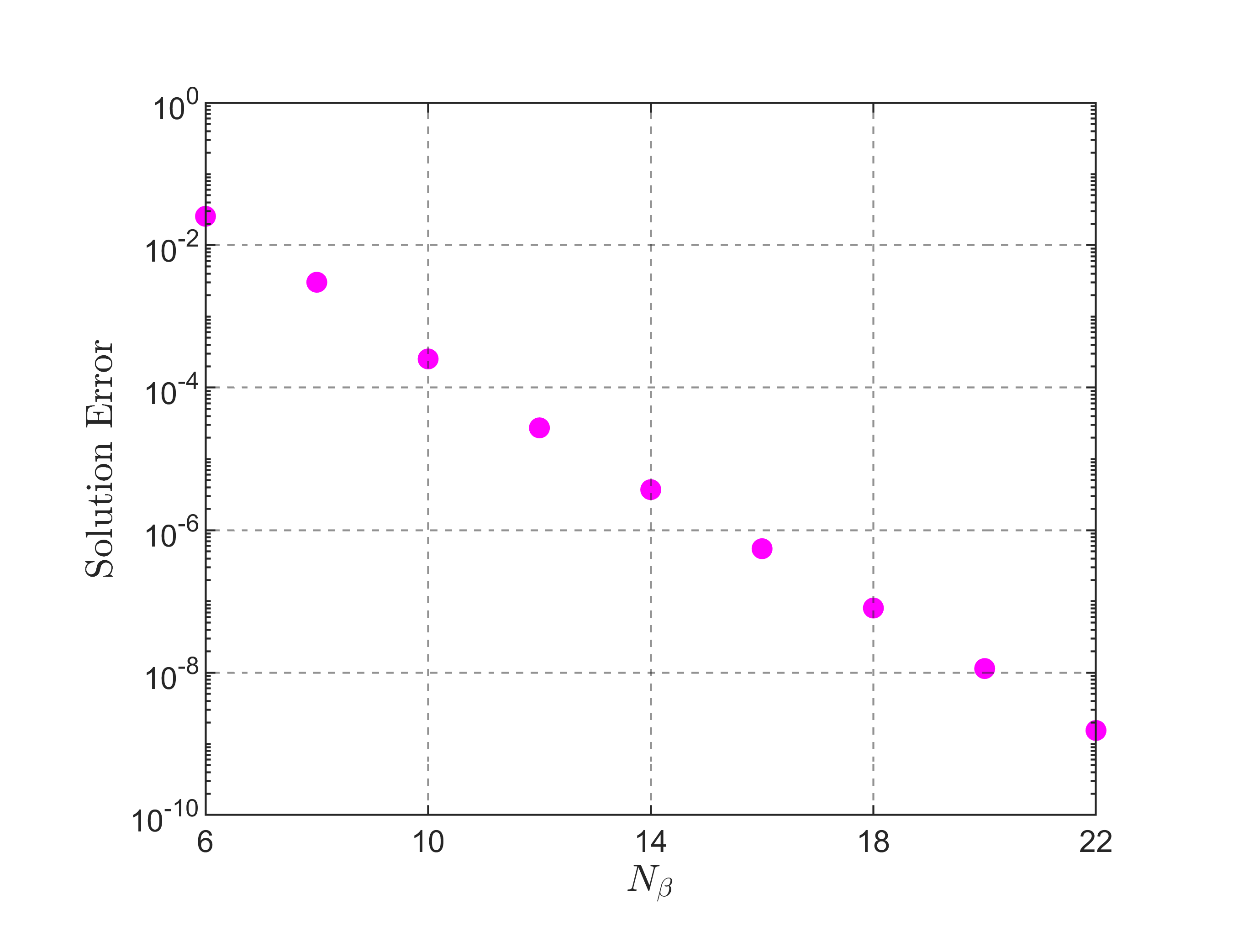
where $p_{OWNS}$ is the pressure computed by OWNS-R, $p_{exact}$ is the pressure computed by the exact OWNS formulation, and $p_{max}$ is the maximum value of the pressure computed using the exact OWNS. The integration region $A$ is the area of the physical domain, not including the far-field damping layers. Fig. 5 shows that the solution error decreases exponentially with increasing $N_{\beta}$ [26] and that reasonable accuracy can be achieved using $O(10)$ recursion parameters.

Second, we consider the example of a turbulent jet. Turbulent jets contain a diverse set of physical phenomena described by multiple modes of the linearized equations, making this a challenging test case and a useful point of comparison between OWNS and PSE. Important types of waves supported by the linearized equations include the Kelvin-Helmholtz instability, which gives rise to large-scale coherent wavepacket structures [42], the Orr mechanism [43, 5], and acoustic waves both trapped within the core of the jet [44, 14] and emitted to the far field.

We consider the specific case of a round jet with Mach number $M=U_{j}/c_{\infty}=0.9$, Reynolds number $Re=\rho_{j}U_{j}D/\mu\approx 1\times 10^{6}$, and temperature ratio $T_{j}/T_{\infty}=1$, where the subscripts $j$ and $\infty$ denote conditions at the jet nozzle exit and in the far-field, respectively, and $D$ is the nozzle geometry. The mean flow about which the Navier-Stokes equations are linearized is obtained from a high-fidelity large-eddy simulation [45]. Following Schmidt et al. [5], we use a turbulent Reynolds number of $Re_{T}=30000$ within the linearized equations. This choice is motivated by recent work showing that using an eddy-viscosity model or reduced effective Reynolds number within linear models improves both near-field [46] and far-field [47] predictions in free-shear flows.

References

- Schmid and Henningson [2000] P. J. Schmid, D. S. Henningson, Stability and Transition in Shear Flows, volume 142, Springer Science & Business Media, 2000.
- Jovanović and Bamieh [2005] M. R. Jovanović, B. Bamieh, Componentwise energy amplification in channel flows, J. Fluid Mech. 534 (2005) 145–183.
- McKeon and Sharma [2010] B. J. McKeon, A. S. Sharma, A critical-layer framework for turbulent pipe flow, J. Fluid Mech. 658 (2010) 336–382.
- Towne et al. [2018] A. Towne, O. T. Schmidt, T. Colonius, Spectral proper orthogonal decomposition and its relationship to dynamic mode decomposition and resolvent analysis, J. Fluid Mech. 847 (2018) 821–867.
- Schmidt et al. [2018] O. T. Schmidt, A. Towne, G. Rigas, T. Colonius, G. A. Brès, Spectral analysis of jet turbulence, J. Fluid Mech. 855 (2018) 953–982.
- Nichols et al. [2017] J. W. Nichols, J. Larsson, M. Bernardini, S. Pirozzoli, Stability and modal analysis of shock/boundary layer interactions, Theoret. Comput. Fluid Dynamics 31 (2017) 33–50.
- Meseguer-Garrido et al. [2014] F. Meseguer-Garrido, J. De Vicente, E. Valero, V. Theofilis, On linear instability mechanisms in incompressible open cavity flow, J. Fluid Mech. 752 (2014) 219–236.
- Citro et al. [2015] V. Citro, F. Giannetti, L. Brandt, P. Luchini, Linear three-dimensional global and asymptotic stability analysis of incompressible open cavity flow, J. Fluid Mech. 768 (2015) 113–140.
- Barkley [2006] D. Barkley, Linear analysis of the cylinder wake mean flow, Europhys. Lett. 75 (2006) 750.
- Nichols and Lele [2011] J. W. Nichols, S. K. Lele, Global modes and transient response of a cold supersonic jet, J. Fluid Mech. 669 (2011) 225–241.
- Edgington-Mitchell et al. [2021] D. Edgington-Mitchell, T. Wang, P. Nogueira, O. Schmidt, V. Jaunet, D. Duke, P. Jordan, A. Towne, Waves in screeching jets, J. Fluid Mech. 913 (2021).
- Crighton and Gaster [1976] D. G. Crighton, M. Gaster, Stability of slowly diverging jet flow, J. Fluid Mech. 77 (1976) 397–413.
- Huerre and Monkewitz [1990] P. Huerre, P. A. Monkewitz, Local and global instabilities in spatially developing flows, Annu. Rev. Fluid Mech. 22 (1990) 473–537.
- Towne et al. [2017] A. Towne, A. V. G. Cavalieri, P. Jordan, T. Colonius, O. Schmidt, V. Jaunet, G. A. Brès, Acoustic resonance in the potential core of subsonic jets, J. Fluid Mech. 825 (2017) 1113–1152.
- Bertolotti and Herbert [1991] F. P. Bertolotti, T. Herbert, Analysis of the linear stability of compressible boundary layers using the pse, Theoret. Comput. Fluid Dynamics 3 (1991) 117––124.
- Malik et al. [1994] M. Malik, F. Li, C.-L. Chang, Crossflow disturbances in three-dimensional boundary layers: nonlinear development, wave interaction and secondary instability, Journal of Fluid Mechanics 268 (1994) 1–36.
- Day et al. [2001] M. Day, N. Mansour, W. Reynolds, Nonlinear stability and structure of compressible reacting mixing layers, Journal of Fluid Mechanics 446 (2001) 375.
- Gudmundsson and Colonius [2011] K. Gudmundsson, T. Colonius, Instability wave models for the near-field fluctuations of turbulent jets, Journal of Fluid Mechanics 689 (2011) 97–128.
- Kreiss and Lorenz [2004] H.-O. Kreiss, J. Lorenz, Initial-boundary value problems and the Navier-Stokes equations, SIAM, 2004.
- Towne et al. [2019] A. Towne, G. Rigas, T. Colonius, A critical assessment of the parabolized stability equations, Theor. Comp. Fluid Dyn. 33 (2019) 359–382.
- Andersson et al. [1998] P. Andersson, D. Henningson, A. Hanifi, On a stabilization procedure for the parabolic stability equations, J. Engr. Mech. 33 (1998) 311–332.
- Chang et al. [1991] C.-L. Chang, M. Malik, G. Erlebacher, M. Hussaini, Compressible stability of growing boundary layers using parabolized stability equations, AIAA Paper 1991-1636 (1991).
- Li and Malik [1996] F. Li, M. R. Malik, On the nature of PSE approximation, Theoret. Comput. Fluid Dynamics 8 (1996) 253–273.
- Cheung and Lele [2009] L. C. Cheung, S. K. Lele, Linear and nonlinear processes in two-dimensional mixing layer dynamics and sound radiation, Journal of Fluid Mechanics 625 (2009) 321–351.
- Towne and Colonius [2013] A. Towne, T. Colonius, Improved parabolization of the Euler equations, AIAA Paper 2013-2171 (2013).
- Towne and Colonius [2015] A. Towne, T. Colonius, One-way spatial integration of hyperbolic equations, Journal of Computational Physics 300 (2015) 844 – 861.
- Towne [2016] A. S. Towne, Advancements in jet turbulence and noise modeling: accurate one-way solutions and empirical evaluation of the nonlinear forcing of wavepackets, Ph.D. thesis, California Institute of Technology, 2016.
- Towne et al. [2021] A. Towne, G. Rigas, E. Pickering, T. Colonius, Efficient global resolvent analysis via the one-way navier-stokes equations. part 1. forced response, arXiv:2111.09269 (2021).
- Rigas et al. [2021] G. Rigas, O. Kamal, A. Towne, T. Colonius, Efficient global resolvent analysis via the one-way navier-stokes equations. part 2. optimal response, arXiv:2111.09273 (2021).
- Hagstrom and Warburton [2004] T. Hagstrom, T. Warburton, A new auxiliary variable formulation of high-order local radiation boundary conditions: corner compatibility conditions and extensions to first-order systems, Wave Motion 39 (2004) 890–901.
- Kamal et al. [2020] O. Kamal, G. Rigas, M. T. Lakebrink, T. Colonius, Application of the one-way navier-stokes (owns) equations to hypersonic boundary layers, in: AIAA AVIATION 2020 FORUM, 2020, p. 2986.
- Briggs [1964] R. J. Briggs, Electron-Stream Interactions with Plasmas, MIT Press, Cambridge, Massachusetts, 1964.
- Kreiss [1970] H. O. Kreiss, Initial boundary value problems for hyperbolic systems, Commun. Pure Appl. Math 23 (1970) 277–298.
- Harris and Hack [2020] S. R. Harris, P. Hack, Well-posed spatial marching of high-amplitude perturbations in viscous shear flows, AIAA Paper 2020-0829 (2020).
- Towne and Colonius [2014] A. Towne, T. Colonius, Continued development of the one-way Euler equations: application to jets, AIAA Paper 2014-2903 (2014).
- Rigas et al. [2017] G. Rigas, T. Colonius, M. Beyar, Stability of wall-bounded flows using one-way spatial integration of Navier-Stokes equations, AIAA Paper 2017-1881 (2017).
- Amestoy et al. [2019] P. R. Amestoy, A. Buttari, J. Y. l’Excellent, T. A. Mary, Bridging the gap between flat and hierarchical low-rank matrix formats: The multilevel block low-rank format, SIAM Journal on Scientific Computing 41 (2019) A1414–A1442.
- Mattsson and Nordström [2004] K. Mattsson, J. Nordström, Summation by parts operators for finite difference approximations of second derivatives, J. Comput. Phys. 199 (2004) 503 – 540.
- Appelo and Colonius [2009] D. Appelo, T. Colonius, A high-order super-grid-scale absorbing layer and its application to linear hyperbolic systems, J. Comput. Phys. 228 (2009) 4200–4217.
- Thompson [1987] K. W. Thompson, Time dependent boundary conditions for hyperbolic systems, J. Comput. Phys. 68 (1987) 1–24.
- Hairer and Wanner [1996] E. Hairer, G. Wanner, Solving ordinary differential equations ii: stiff and differential-algebraic problems, 1996.
- Jordan and Colonius [2013] P. Jordan, T. Colonius, Wave packets and turbulent jet noise, Annu. Rev. Fluid Mech. 45 (2013) 173–195.
- Tissot et al. [2017] G. Tissot, M. Zhang, F. C. Lajús, A. V. G. Cavalieri, P. Jordan, Sensitivity of wavepackets in jets to nonlinear effects: the role of the critical layer, J. Fluid Mech. 811 (2017) 95–137.
- Tam and Hu [1989] C. K. W. Tam, F. Q. Hu, On the three families of instability waves of high-speed jets, J. Fluid Mech. 201 (1989) 447–483.
- Brès et al. [2018] G. A. Brès, P. Jordan, M. Le Rallic, V. Jaunet, A. V. G. Cavalieri, A. Towne, S. K. Lele, T. Colonius, O. T. Schmidt, Importance of the nozzle-exit boundary-layer state in subsonic turbulent jets, J. Fluid Mech. 851 (2018) 83–124.
- Pickering et al. [2021a] E. Pickering, G. Rigas, O. T. Schmidt, D. Sipp, T. Colonius, Optimal eddy viscosity for resolvent-based models of coherent structures in turbulent jets, J. Fluid Mech. 917 (2021a).
- Pickering et al. [2021b] E. Pickering, A. Towne, P. Jordan, T. Colonius, Resolvent-based modeling of turbulent jet noise, J. Acoust. Soc. Am. 150 (2021b) 2421–2433.
- Cavalieri et al. [2012] A. V. G. Cavalieri, P. Jordan, T. Colonius, Y. Gervais, Axisymmetric superdirectivity in subsonic jets, J. Fluid Mech. 704 (2012) 388–420.
- Chen and Towne [2021] Z. Chen, A. Towne, An azimuthal fourier domain formulation of the Ffowcs Williams and Hawkings equation, J. Acoust. Soc. Am. 150 (2021) 1967–1978.
- Towne et al. [2017] A. Towne, G. A. Brès, S. K. Lele, A statistical jet-noise model based on the resolvent framework, AIAA Paper 2017-3406 (2017).
- Rigas et al. [2017] G. Rigas, O. T. Schmidt, T. Colonius, G. A. Brès, One way navier-stokes and resolvent analysis for modeling coherent structures in a supersonic turbulent jet, AIAA Paper 2017-4046 (2017).
- Suzuki and Colonius [2006] T. Suzuki, T. Colonius, Instability waves in a subsonic round jet detected using a near-field phased microphone array, J. Fluid Mech. 565 (2006) 197–226.
- Haj-Hariri [1994] H. Haj-Hariri, Characteristics analysis of the parabolized stability equations, Stud. Appl. Math. 92 (1994) 41–53.
- Ma and Zhong [2003] Y. Ma, X. Zhong, Receptivity of a supersonic boundary layer over a flat plate. part 1. wave structures and interactions, Journal of Fluid Mechanics 488 (2003) 31.
- Knisely and Zhong [2019] C. P. Knisely, X. Zhong, Sound radiation by supersonic unstable modes in hypersonic blunt cone boundary layers. I. Linear stability theory, Phys. Fluids 31 (2019) 024103.
- Fedorov [2011] A. Fedorov, Transition and stability of high-speed boundary layers, Annu. Rev. Fluid Mech. 43 (2011) 79–95.
- Fedorov and Tumin [2011] A. Fedorov, A. Tumin, High-speed boundary-layer instability: Old terminology and a new framework, AIAA J. 49 (2011) 1647–1657.
- Ribeiro et al. [2020] J. H. M. Ribeiro, C.-A. Yeh, K. Taira, Randomized resolvent analysis, Phys. Rev. Fluids 5 (2020) 033902.
- Martini et al. [2021] E. Martini, D. Rodríguez, A. Towne, A. V. G. Cavalieri, Efficient computation of global resolvent modes, J. Fluid Mech. 919 (2021).
- Farghadan et al. [2021] A. Farghadan, A. Towne, E. Martini, A. V. G. Cavalieri, A randomized time-domain algorithm for efficiently computing resolvent modes, AIAA Paper 2021-2896 (2021).