Explaining GNN over Evolving Graphs using Information Flow
Abstract
Graphs are ubiquitous in many applications, such as social networks, knowledge graphs, smart grids, etc.. Graph neural networks (GNN) are the current state-of-the-art for these applications, and yet remain obscure to humans. Explaining the GNN predictions can add transparency. However, as many graphs are not static but continuously evolving, explaining changes in predictions between two graph snapshots is different but equally important. Prior methods only explain static predictions or generate coarse or irrelevant explanations for dynamic predictions. We define the problem of explaining evolving GNN predictions and propose an axiomatic attribution method to uniquely decompose the change in a prediction to paths on computation graphs. The attribution to many paths involving high-degree nodes is still not interpretable, while simply selecting the top important paths can be suboptimal in approximate the change. We formulate a novel convex optimization problem to optimally select the paths that explain the prediction evolution. Theoretically, we prove that the existing method based on Layer-Relevance-Propagation (LRP) is a special case of the proposed algorithm when an empty graph is compared with. Empirically, on seven graph datasets, with a novel metric designed for evaluating explanations of prediction change, we demonstrate the superiority of the proposed approach over existing methods, including LRP, DeepLIFT, and other path selection methods.
Introduction
Graph neural networks (GNN) are now the state-of-the-art method for graph representation in many applications, such as molecule property prediction (Wu et al. 2018), social network modeling (Kipf and Welling 2017), pose estimation in computer vision (Yang et al. 2021), knowledge graph embedding (Wang et al. 2019), and recommendation systems (Ying et al. 2018). It is desirable to make the GNN predictions transparent to humans (Ying et al. 2019; Schnake et al. 2020; Pope et al. 2019; Ren et al. 2021; Liu et al. 2021). For example, a user may want to know why a particular recommendation is made to ensure that the recommendation does not breach personal private information (e.g., age and gender); for sanity check, a prediction of pose must be based on salient configurations of human landmarks rather than backgrounds. However, the graph dependencies intertwine a GNN prediction with many nodes several hops away through multiple paths, making the identification of the salient contributors challenging. To explain GNN predictions on a static graph, there are local or global explanation approaches (Yuan et al. 2020b). Given a trained GNN model, local explanations explain a GNN prediction by selecting salient subgraphs (Ying et al. 2019), nodes, or edges (Schnake et al. 2020). Global methods (Yuan et al. 2020a; Vu and Thai 2020; Huang et al. 2020) learn simpler surrogate models to approximate the target GNN and generate explaining models or instances.
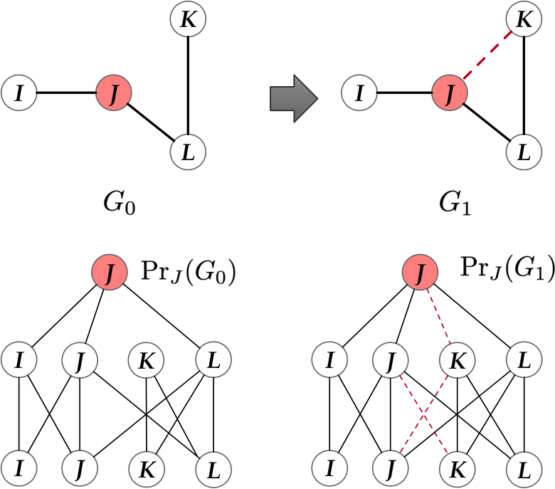
In the real world, graphs are usually evolving. For example, pose estimation from videos needs to handle series of graphs representing landmarks of human bodies; knowledge graphs and social networks are undergoing constant updates. GNN predictions can change with respect to the evolving graph. To explain prediction changes is to identify salient graph changes contributing to the prediction changes, so that humans can understand what causes the change (see Figure 1) and how GNN changes its predictions.
Given a graph and assuming multi-class prediction, let be the logits of classes of the node . The classes are indexed by (in general, we let lower-case index the neurons of a node). The predicted class distribution is ( is the probability of class ). On a static graph , or will be explained (Ying et al. 2019; Huang et al. 2020), while when evolves to , the difference between and (or and ) needs to be explained.
Perturbation and counterfactual explanation methods (Dhurandhar et al. 2018; Lucic et al. 2021) can attribute a static prediction to individual edges or nodes by searching the optimal change to the input graph, while we are handling arbitrary given graph evolution from to and discovering the cause of the change. We focus on attributing prediction changes to GNN propagation paths where information flows (see Figure 1, top). The axiomatic attribution method GNN-LRP (Schnake et al. 2020) handles each class independently given a static graph and cannot explain arbitrary change in the distribution of multiple classes. DeepLIFT (Shrikumar, Greenside, and Kundaje 2017) can explain the log-odd between two classes only (the original and the new predicted classes), which does not fully capture the change in a multi-class distribution. For example, let classes 1 and 2 be the classes with the highest probabilities for the same node appearing in the graphs and , respectively. One can construct an example multi-class distribution so that and , where the log-odd is positive but the positive contributions of the salient factors to the log-odd cannot explain the reduction in the predicted class probability on .
Lastly, to obtain simple explanations, prior methods select a few edges or nodes with the highest importance (Ying et al. 2019; Shrikumar, Greenside, and Kundaje 2017; Lundberg and Lee 2017; Schnake et al. 2020). However, ranking based on importance can be sub-optimal. For example, let the change in a logit be 2, which is attributed to three edges as . If no more than two edges can be selected, the simplest and most accurate approximation is , rather than , , or found based on the magnitudes of the contributions.
To address the above challenges, we design an algorithm to explain the change in the probability using a small number of propagation paths that reflect the change of information flow of GNN computation. We focus on when a single edge is added, with multiple added edges as a simple extension11 1 Edge removals can be handled similarly, but a mixture of addition and removal need a careful analysis and is left as future work.. We first identify the paths containing the added edge, as other paths make no contributions to the change of prediction. We attribute the KL-divergence between two multi-class distributions, rather than static or log-odds of posteriors, to explain the prediction change. The softmax and the KL-divergence are non-linear everywhere and are thus not amenable to the prior axiomatic attribution methods, which are inherently linear. Rather, we approximate the KL-divergence in two steps: i) decomposing the changes in the logits over all classes to the altered paths to allow a unique and linear attribution; ii) we design a convex optimization problem to select important paths that can optimally approximate the non-linear KL-divergence.
The proposed algorithm goes beyond seeking what causes the change in prior works (Ying et al. 2019; Lucic et al. 2021) and explains how changing connectivity leads to the change in the information flow of GNN computation graphs. Theoretically, we prove that GNN-LRP (Schnake et al. 2020) is a special case of the proposed attribution method starting from a graph without any edge. Empirically, as prior evaluation metrics do not align well with the quality of the explanations of prediction changes, we propose a novel metric based on KL-divergence. We show that solving the convex optimization can select a good portfolio of contributing paths that jointly approximate the change better than ranking-based and linear programming approaches.
Preliminaries and problem definition
Graph neural networks. Assume that we have a trained GNN of layers that predicts the class distribution of each node on a graph . Let be the neighbors of node . On layer , and for node , GNN computes using messages sent from its neighbors:
| (1) | |||
| (2) |
aggregates the messages from all neighbors and can be the element-wise sum, average, or maximum of the incoming messages. maps to , using or a multi-layered perceptron with parameters . For layer , we let NONLINEAR be the ReLU. At the input layer, node feature vector for is regarded as . At layer , the logits are , whose -th element denotes the logit of the class . is mapped to the class distribution through softmax. The class is predicted for node .
Evolving graphs. Let denote the initial graph with edges and nodes . Let denote the graph that evolves from . We assume that evolves into with edges added while the nodes and the node features remain the same. Let denote the set of edges added, . When the graph evolves to , let denote the set of target nodes, each with a change in its class distribution to be explained: .
Path-based explanations of GNN. The GNN prediction at node is generated by a computation graph, which is a spanning tree of rooted at of depth . The leaf nodes contain neurons from the input layer () and the root node contains neurons of the output layer () (see Figure 1). The trees completely represent Eq. (2) where messages are passed along the paths traversing from leaves to roots. Let a path be , where and represent any two adjacent nodes on the path and is designated as the root. For a GNN with layers, the paths are sequences of nodes and we let be the set of all such paths. Let be the paths ending at .
The set contains all paths with at least one edge that is an added edge, and therefore completely explains the change in . In the example in Figure 1, . However, the contribution of the paths in is unknown. Furthermore, if the paths in are too many, is not interpretable. We define a path-based explanation of a change in as a small subset of closely approximating the change. Attribution to paths can reveal the details of the change in the information flow of GNN, which cannot be found by the coarse-grained attribution to altered edges (Dhurandhar et al. 2018; Lucic et al. 2021).
AxiomPath-Convex: optimal convex attribution of prediction change to paths
Most GNN explanation methods attribute a static prediction to nodes or edges on a static graph (Ying et al. 2019; Schnake et al. 2020). Formally, or for class is decomposed into contributions from multiple nodes and edges. Counterfactual explanations of GNN (Lucic et al. 2021) only identify altered edges, rather than changes in the information flow among the neurons, as the cause of the change, In (Shrikumar, Greenside, and Kundaje 2017), the log-odd of the original and new predicted classes and is used to measure the changes in when a fixed baseline graph evolves to a graph . Besides being unable to handle evolution from an arbitrary to , a more fundamental issue is that the two probabilities and are not comparable due to the normalization in softmax and the log-odd does not capture distribution change. For example, with three classes, let and . Then the maximal probabilities are the same for two different classes and the log-odd is , indicating no change. In fact, can be greater than and the log-odd is positive, giving a wrong sense that class is more likely than , although the predicted class changes from to . A metric and an explanation faithfully reflecting the direction and amount of change is yet to be invented.
Decomposing KL-divergence to path contributions
KL-divergence is a well-defined distance metric of probability distributions. In (Suermondt 1992; Ying et al. 2019), KL-divergence is used to measure the approximation quality of a static predicted distribution . However, there is no prior work that attributes KL-divergence to paths of information flow of GNN. We will explain the KL-divergence using paths.
For a target node , let the difference between its logits calculated on graphs and be . The KL-divergence between two predicted class distributions is
| (3) | ||||
where for . In Eq. (3), we are adding up the log-odds of the probabilities of the same class between two predicted distributions, rather than comparing the probabilities of two different classes from two distributions as done by DeepLIFT.
Assume that the change in the logits can be linearly and exactly attributed to altered propagation paths in when evolves into . Formally, and , where is the contribution of the -th altered path to . Note that the paths in the summation is the same for all . Accordingly, the KL-divergence becomes
| (4) |
In the next section we will show how to find the altered paths and calculate .
In Eq. (4), the number of paths () can be quite large, especially when adding an edge to a node with high degree, Using Eq. (4) to explain the KL-divergence is not interpretable. Consider selecting a subset of paths from . The collection of paths can be considered as the computation graph for node on a partially evolved graph between and . For example, in Figure 1, we can take with .

With the partial contributions from the paths, the logits on the graph partially evolved from is . Here we abuse the notation to represent and index a path. By replacing with , Eq. (4) becomes
| (5) |
This is the KL-divergence between two distributions and and has the minimum of 0. If it is close to 0, then the contribution from can move to (or to ) using paths, when paths have significant redundancy. The idea is shown in Figure 2. It is important to add the contributions to , , to make sure that the added paths will approximate starting from . If the contributions were to be added to a different starting graph (a commonly found example is the empty graph), the KL-divergence in Eq. (5) will not explain the change from to .
We formulate an optimization problem to select . Let , , be optimization variables representing the probabilities of selecting path into . We solve the following nonlinear minimizing problem:
| (6) | |||||
| s.t. | (7) |
The first term is linear in and the second term is the composition of a log-sum-exp function (convex and non-decreasing) and a linear function of . The constraint function is linear in . Therefore, the optimization problem is convex and has a unique optimal solution given the constant . In going from Eq. (5) to the objective, we ignore the constants , , and . The linear constraint is to ensure the total probabilities of the selected edges is . Note the similarity between the optimization problem and the minimization of multi-class logistic regression: can be regarded as regression parameters and the paths as features. After obtaining , we rank the paths based on and include the top paths in .
Background on DeepLIFT
It remains to calculate for all paths . We extend DeepLIFT to attribute prediction change to of the paths in . Let the neuron be computed by , with inputs neurons . Given the reference activations at layer , we can calculate the reference activation . The difference-from-reference is and , . The 0 in parentheses indicates the original input and the 1 indicates the changed input. The contribution of neuron to is denoted by such that and is preserved by the sum of all contributions.
DeepLIFT for GNN
We let the reference activations be computed by the GNN on the graph . We assume that there is just one edge added to to obtain since the more general case with multiple added edges can be decomposed into multiple steps of adding one edge. Let and represent any adjacent nodes in a path, where is closer to the root .
Difference-from-reference of neuron activation and logits. For a path in , let denote the neurons of the node at layer . For example, if , represents the neurons of node at layer and represents the neurons of node at layer . Given a path , let . When , the reference activation of is . While when , the reference activation of is zero, because the message of cannot be passed along the path to in , since the edge must be added to to connect to in the path. We thus calculate the difference-from-reference of neurons at each layer as follows:
For example, in Figure 3, the added edge is . For the path in , . and , because in , the neuron at layer cannot pass message to the neuron at the output layer along the path in .
The change in the logits can be handled similar to .
Obtain multiplier of each neuron to its immediate successor. The linear rule and the rescale rule designed by the DeepLIFT can be used for backpropagation to obtain the multiplier of each neuron to its immediate successor.
We choose element-wise sum as the function to ensure that the attribution by DeepLIFT can preserve the total change in the logits such that . Then, is rewritten into the following form.
| (11) |
where denotes the element of the matrix that links neuron to neuron . Therefore, we can obtain the multiplier of the neuron to its immediate successor neuron .
| (12) |
Note that the output of GNN model is , thus . We can obtain the multiplier of each neuron to its immediate successor in the path according to Eq. (12) by letting go from to . After obtaining the , according to the chain rule, we can obtain .
Calculate the contribution of each path. For the path in , we obtain the contribution of the path by summing up the input neurons’ contributions: , where indexes the neurons of the input (a leaf node in the computation graph of the GNN).
Theorem 1.
The GNN-LRP is a special case if the reference activation is set to the empty graph.
See the Appendix for a proof.
Experiments
| Datasets | Classes | Nodes | Edges | Edge/Node | Features |
| Cora | 7 | 2,708 | 10,556 | 3.90 | 1,433 |
| Citeseer | 6 | 3,321 | 9,196 | 2.78 | 3,703 |
| PubMed | 3 | 1,9717 | 44,324 | 2.24 | 500 |
| Amazon-C | 10 | 13,752 | 574,418 | 41.77 | 767 |
| Amazon-P | 8 | 7,650 | 287,326 | 37.56 | 745 |
| Coauthor-C | 15 | 18,333 | 327,576 | 17.87 | 6,805 |
| Coauthor-P | 5 | 34,493 | 991,848 | 28.76 | 8,415 |
Datasets and tasks. We select graph datasets that are suitable for node classification. Certain datasets used in prior GNN explanation works are not applicable. For example, it is hard to create evolving molecule graphs (Debnath et al. 1991; Wu et al. 2018) and dependency parse trees (Socher et al. 2013; Schnake et al. 2020) while maintaining the syntactic integrity of the graphs. Besides, these datasets are majorly used for graph classification rather than node classification. Second, the motif-based patterns (grids vs. trees) of the synthetic graphs (Ying et al. 2019) cannot be explained by simple paths. Therefore, we adopt 7 graph datasets from three real-world applications for evaluation (see Table 1 and the Appendix for the details).
Baselines. We adopt the following methods as baselines.
- •
Gradient (Grad) employs the gradients of the logits of class of target node with respect to individual edges as edge importance. Path importance is the sum of absolute gradients of the edges of a path. Paths are ranked and selected from the existing and newly added paths.
- •
GNN-LRP adopts the back-propagation attribution method LRP to GNN (Schnake et al. 2020). However, it only attributes the single predicted class probability to input neurons and the original graph is not accounted for. Path relevance is calculated in the same way as specified in (Schnake et al. 2020) and the path ranking and selection is done as in Grad.
- •
DeepLIFT (Shrikumar, Greenside, and Kundaje 2017) is the most relevant baseline as it can explain the difference between the predicted class probabilities from two graphs. It can handle zero activations ignored by GNN-LRP. However, it attributes the log-odds between the original and new predicted classes to neurons and does not directly apply to GNN. We design the GNN version of DeepLIFTGNN by branching out to all neurons of all neighbors of a node during back-propagation. Then we take the sum of contributions of the input neurons at node to class as the contribution of the unique path from to for that class. Lastly, the difference between each path’s contributions to the new and original predicted classes is used to rank and select paths in .
- •
AxiomPath-Topk is a variant of AxiomPath-Convex, without solving the convex programming. Rather, it selects paths with top contributions to all classes . The path ranking and selection are the same as DeepLIFT.
- •
AxiomPath-Linear solves the optimization problem in Eq. (6) without the log term, leading to a linear programming problem. The resulting optimal is processed in the same way as AxiomPath-Convex.
Certain prior methods are not suitable as baselines. CAM and Grad-CAM are not applicable since they cannot explain node classification models (Yuan et al. 2020b). PGExplainer and SubgraphX find subgraphs as explanations of static predictions while being not comparable with path-based explanations. GNNExplainer finds the importance of individual edges that multiplex an edge’s contributions to multiple paths of information flow. Simply combining edge importance to select paths leads to much worse fidelity and thus GNNExplainer is not a relevant baseline.
Experimental setup. For each graph dataset, we first train and fix a GNN for node classification on the labeled training set. Randomly selected edges are added to simulate the graph evolution. At the end of the evolution, the set of target nodes with a different prediction is collected and the change in each target node is explained using the various methods. The target nodes are grouped based on the number of added paths for the results to be comparable. For each group, we let (the number of selected edges) range in a pre-defined set to create 10 levels of explanation complexity (). We use SCS solver in the cvxpy library to solve the constrained convex optimization problem. We run the evolution and explanation for times to calculate the means and standard deviations of the following fidelity metric over target nodes. (see the Appendix for more details)
Evaluation Metrics. Even though explanation visualization allows humans to judge whether the explanations are reasonable, it cannot objectively evaluate the explanations. Instead, we design the following new metric to evaluate fidelity in explaining changes in class distributions:
where is the class distribution computed on the computation graph for with the selected paths removed. Intuitively, if indeed contains the important paths to turn into , the less information the remaining paths can propagate, the more similar is to , and the smaller the ratio. At one extreme, so that the numerator is just (nothing is removed) and the ratio is 1. At the other extreme, includes all added paths and degrades to and the ratio is 0. The denominator is for normalization since the total change can be of different scales for different . We intentionally design this metric to differ from the objective function in Eq. (6) so that AxiomPath-Convex has less privilege. For fairness, we ensure the same number of edges are removed from the same set of paths, so that the number of remaining paths is the same for all methods.
Performance evaluation and comparison
Path importance on real-world datasets. In Figure 4, we demonstrate the effectiveness of the salient path selection of AxiomPath-Convex. For each dataset, we report the mean fidelity over 10 random experiments and over target nodes whose predictions are altered (standard deviations are reported in the Appendix). The lower the fidelity, the better (since we intend to remove the important paths identified by ). From the figure, we can see that AxiomPath-Convex has the smallest fidelity over all levels of explanation complexities and over all datasets. On four datasets (Cora, Citeseer, Amazon-C, and Amazon-P), the gap between AxiomPath-Convex and the runner-up (DeepLIFT) is significant. On the remaining three datasets, the gap is less significant but still not ignorable. The third best baseline is AxiomPath-Linear, indicating the power of using optimization for selecting explaining paths, and more importantly, the need to approximate the KL-divergence in full using non-linear convex optimization. GNN-LRP lacks consistency: on all datasets, it has increasing fidelity when the complexity level goes up after some points. AxiomPath-Topk underperforms AxiomPath-Linear, indicating that paths must be selected jointly rather than independently. Furthermore, though descending at a slower pace, AxiomPath-Topk and AxiomPath-Linear consistently decreases the fidelity as more important paths are identified, indicating the “consistency” of the proposed attribution method shared by the AxiomPath- family. Grad always (and sometimes for GNN-LRP) fails to find the right paths to explain the change, as they are designed for static graphs.
Preserving changes during attributions.
Edges randomly selected are added or deleted to simulate the graph evolution and the parameters for the GNN model are randomly generated. For the target node in , if the difference is less than , we regard the change as successfully preserved. We calculate the percentage of successful preservation among . Figure 5) shows that the attribution preserves the change in the logits 100%.
Running time overhead of convex optimization. We plot the base running time of searching paths in and attribution vs. the running time of optimization afterwards. From Figure 6, we can see that in most cases when the number of new paths is not extremely large, the optimization step takes a reasonable amount of time compared to the base running time. However, there are two exceptions on the Amazon dataset when the number of new paths is large. We argue that’s because the off-the-shelf optimizer in scipy is used and a customized optimizer can reduce the running time, by early stopping.
Related work
Regarding what about GNN is explained, there are methods explaining the predicted class distribution of graphs or nodes using mutual information as the objective function (Ying et al. 2019). Other works explained the logit or probability of a single class (Schnake et al. 2020). CAM, GradCAM, GradInput, SmoothGrad, IntegratedGrad, Excitation Backpropagation, and attention models are evaluated in (Wiltschko et al. 2020; Pope et al. 2019) with the focus on explaining the prediction of a single class. The closest works are DeepLIFT (Shrikumar, Greenside, and Kundaje 2017) and counterfactual explanations (Lucic et al. 2021), but they only explain the changes in a single class rather than in class distributions involving more than two classes.
To compose an explanation, edges (Schnake et al. 2020; Ying et al. 2019; Faber, K. Moghaddam, and Wattenhofer 2021; Shrikumar, Greenside, and Kundaje 2017; Lucic et al. 2021) and nodes (Pope et al. 2019) have been used to construct explanations. Simple surrogate models (Huang et al. 2020; Vu and Thai 2020) or generated samples (Yuan et al. 2020a) have been used. These works cannot expose the change in information flow leading to prediction changes.
Selecting salient elements to compose an explanation is less focused. Most work simply selects nodes or edges with the highest importance scores (Schnake et al. 2020; Ying et al. 2019; Faber, K. Moghaddam, and Wattenhofer 2021) with the underlying assumption that the nodes/edges contributions are independent. Negative contributions were turned into absolute values or norms (Pope et al. 2019), or even be discarded (Shrikumar, Greenside, and Kundaje 2017), and it is not clear how negative importance scores are handled in (Wiltschko et al. 2020). Our convex path selection addresses both positive and negative contributions while considering the joint effect of path contributions.
Most of the prior work evaluates the faithfulness of the explanations, mainly using the closeness of the approximating prediction to the explained prediction. To explain prediction changes, faithfulness should be evaluated based on approximation of the change. Our metric is based on KL-divergence and designed specifically for prediction distribution changes.
Conclusions
We studied the problem of explaining change in GNN predictions over evolving graphs. We addressed the issues of prior works, such as irrelevant explained quantity, lack of optimality, and axiomatic attribution for GNN. The proposed algorithm can decompose the change to information flows in the computation graphs of GNN and optimally select a small subset of paths to optimally explain the change in prediction change (using an argument of convexity). Experimentally results showed the superiority of the proposed method over state-of-the-art baselines. In the future work, we plan to address the situation when the edges are removed and added simultaneously.
References
- Debnath et al. (1991) Debnath, A. K.; de Compadre, R. L. L.; Debnath, G.; Shusterman, A. J.; and Hansch, C. 1991. Structure-activity relationship of mutagenic aromatic and heteroaromatic nitro compounds. correlation with molecular orbital energies and hydrophobicity.
- Dhurandhar et al. (2018) Dhurandhar, A.; Chen, P.-Y.; Luss, R.; Tu, C.-C.; Ting, P.; Shanmugam, K.; and Das, P. 2018. Explanations Based on the Missing: Towards Contrastive Explanations with Pertinent Negatives. In Proceedings of the 32nd International Conference on Neural Information Processing Systems, 590–601.
- Faber, K. Moghaddam, and Wattenhofer (2021) Faber, L.; K. Moghaddam, A.; and Wattenhofer, R. 2021. When Comparing to Ground Truth is Wrong: On Evaluating GNN Explanation Methods. In Proceedings of the 27th ACM SIGKDD Conference on Knowledge Discovery & Data Mining, KDD ’21.
- Huang et al. (2020) Huang, Q.; Yamada, M.; Tian, Y.; Singh, D.; Yin, D.; and Chang, Y. 2020. GraphLIME: Local interpretable model explanations for graph neural networks. arXiv preprint arXiv:2001.06216.
- Kipf and Welling (2017) Kipf, T. N.; and Welling, M. 2017. Semi-supervised classification with graph convolutional networks. In International Conference on Learning Representations (ICLR).
- Liu et al. (2021) Liu, M.; Luo, Y.; Wang, L.; Xie, Y.; Yuan, H.; Gui, S.; Yu, H.; Xu, Z.; Zhang, J.; Liu, Y.; Yan, K.; Liu, H.; Fu, C.; Oztekin, B.; Zhang, X.; and Ji, S. 2021. DIG: A Turnkey Library for Diving into Graph Deep Learning Research. arXiv preprint arXiv:2103.12608.
- Lucic et al. (2021) Lucic, A.; ter Hoeve, M.; Tolomei, G.; Rijke, M.; and Silvestri, F. 2021. CF-GNNExplainer: Counterfactual Explanations for Graph Neural Networks. ArXiv, abs/2102.03322.
- Lundberg and Lee (2017) Lundberg, S. M.; and Lee, S.-I. 2017. A Unified Approach to Interpreting Model Predictions. In Advances in Neural Information Processing Systems 30, 4765–4774.
- Pope et al. (2019) Pope, P. E.; Kolouri, S.; Rostami, M.; Martin, C. E.; and Hoffmann, H. 2019. Explainability Methods for Graph Convolutional Neural Networks. In 2019 IEEE/CVF Conference on Computer Vision and Pattern Recognition (CVPR).
- Ren et al. (2021) Ren, J.; Li, M.; Liu, Z.; and Zhang, Q. 2021. Interpreting and Disentangling Feature Components of Various Complexity from DNNs. In Proceedings of the 38th International Conference on Machine Learning.
- Schnake et al. (2020) Schnake, T.; Eberle, O.; Lederer, J.; Sch¨utt, S. N. K. T.; M¨uller, K.-R.; and Montavon, G. 2020. Higher-order explanations of graph neural networks via relevant walks.
- Shrikumar, Greenside, and Kundaje (2017) Shrikumar, A.; Greenside, P.; and Kundaje, A. 2017. Learning Important Features Through Propagating Activation Differences. In ICML.
- Socher et al. (2013) Socher, R.; Perelygin, A.; Wu, J. Y.; Chuang, J.; Manning, C. D.; Ng, A. Y.; and Potts, C. 2013. Recursive deep models for semantic compositionality over a sentiment treebank. In Empirical Methods in Natural Language Processing.
- Suermondt (1992) Suermondt, H. J. 1992. Explanation in Bayesian Belief Networks. Ph.D. thesis.
- Vu and Thai (2020) Vu, M. N.; and Thai, M. 2020. PGM-Explainer: Probabilistic Graphical Model Explanations for Graph Neural Networks. In NeurIPS.
- Wang et al. (2019) Wang, H.; Zhang, F.; Zhang, M.; Leskovec, J.; Zhao, M.; Li, W.; and Wang, Z. 2019. Knowledge-Aware Graph Neural Networks with Label Smoothness Regularization for Recommender Systems. In Proceedings of the 25th ACM SIGKDD International Conference on Knowledge Discovery & Data Mining.
- Wiltschko et al. (2020) Wiltschko, A. B.; Sanchez-Lengeling, B.; Lee, B.; Reif, E.; Wei, J.; McCloskey, K. J.; Colwell, L.; Qian, W.; and Wang, Y. 2020. Evaluating Attribution for Graph Neural Networks. In Advances in Neural Information Processing Systems 33.
- Wu et al. (2018) Wu, Z.; Feinberg, B. R. E. N.; Gomes, J.; Geniesse, C.; Pappu, A. S.; Leswing, K.; and Pande, V. S. 2018. Moleculenet: a benchmark for molecular machine learning.
- Yang et al. (2021) Yang, Y.; Ren, Z.; Li, H.; Zhou, C.; Wang, X.; and Hua, G. 2021. Learning Dynamics via Graph Neural Networks for Human Pose Estimation and Tracking. CVPR.
- Ying et al. (2019) Ying, R.; Bourgeois, D.; You, J.; Zitnik, M.; and Leskovec, J. 2019. GNNExplainer: Generating Explanations for Graph Neural Networks. In Neural Information Processing Systems.
- Ying et al. (2018) Ying, R.; He, R.; Chen, K.; Eksombatchai, P.; Hamilton, W. L.; and Leskovec, J. 2018. Graph Convolutional Neural Networks for Web-Scale Recommender Systems. In KDD.
- Yuan et al. (2020a) Yuan, H.; Tang, J.; Hu, X.; and Ji, S. 2020a. XGNN: Towards Model-Level Explanations of Graph Neural Networks.
- Yuan et al. (2020b) Yuan, H.; Yu, H.; Gui, S.; and Ji, S. 2020b. Explainability in Graph Neural Networks: A Taxonomic Survey. ArXiv, abs/2012.15445.
Appendix
Proof of Theorem 1
Proof.
Considering the path on the graph , for the DeepLIFT on the graph, we let the reference activations be set to the empty graph. Then, the reference activation of is zero. Thus, . While, for the GNN-LRP method when , on the message passing layers, , we note that represents the allocation rule of neuron to its predecessor neuron in the GNN-LRP method. The contribution of this path is
∎
Datasets
- •
Citeseer, Cora, and PubMed (Kipf and Welling 2017): each node is a paper with a bag-of-words feature vector, and nodes are connected by the citation relationship. The goal is to predict the research area of each paper.
- •
Amazon-Computer (Amazon-C) and Amazon-Photo (Amazon-P) (shchur2018pitfalls): segments of the Amazon co-purchase graph, where nodes represent products and edges indicate that two products are frequently purchased together, node features are the bag-of-words vectors of the product reviews.
- •
Coauthor-Computer and Coauthor-Physics: co-authorship graphs based on the Microsoft Academic Graph from the KDD Cup 2016 Challenge. We represent authors as nodes, that are connected by an edge if they co-authored a paper (shchur2018pitfalls). Node features represent paper keywords for each author’s papers.
Experimental setup
We choose element-wise sum as the function to ensure that the attribution by DeepLIFT can preserve the total change in the logits. We train the GNN model with two layers and three layers on seven datasets and fix these model parameters. 200 edges randomly selected are added to simulate the graph evolution. To show that as increases, is gradually approaching , we let n gradually increase. Moreover, is different for the different nodes in , so we choose according to . If , if and if
Standard deviation for
From Figure 7, we can see that although on the PubMed dataset, the standard deviation of AxiomPath-Convex is higher than the standard deviation of AxiomPath-Topk when the Explanation complexity level is 9 or 10, AxiomPath-Convex has the smallest standard deviation over all levels of explanation complexities on six datasets (Cora, Citeseer, Amazon-C, Amazon-P, Coauthor-Computer and Coauthor-Physics). Thus, AxiomPath-Convex has the best performance.
Performance evaluation and comparison
In the main texts, we show the mean Fidelity over all datasets and the number of layers of the fixed GNN model is two. When the number of GNN model layers is three, we also run the evolution and explanation for ten times to calculate the means and standard deviations of the Fidelity over target nodes.
When the number of GNN model layers is three, AxiomPath-Convex can still perform better than other baselines. AxiomPath-Convex has the smallest fidelity over all levels of explanation complexities and over all datasets. AxiomPath-Convex has the smallest standard deviation over all levels of explanation complexities on five datasets (Cora, Citeseer, Amazon-C, Amazon-P and Coauthor-Computer). In Figure 8 and Figure 9, we demonstrate the effectiveness of the salient path selection of AxiomPath-Convex.
Running time overhead of convex optimization.
In the main texts, we plot the base running time of searching added path and attribution vs. the running time of optimization afterwards on the Amazon-Photo and Coauthor-Physics datasets. In Figure 10, we plot the running time on the other five datasets.
We can see that in most cases when the number of new paths is not extremely large, the optimization step takes a reasonable amount of time compared to the base running time.