Minimum Resource Threshold Policy Under Partial Interference
Abstract
When developing policies for prevention of infectious diseases, policymakers often set specific, outcome-oriented targets to achieve. For example, when developing a vaccine allocation policy, policymakers may want to distribute them so that at least a certain fraction of individuals in a census block are disease-free and spillover effects due to interference within blocks are accounted for. The paper proposes methods to estimate a block-level treatment policy that achieves a pre-defined, outcome-oriented target while accounting for spillover effects due to interference. Our policy, the minimum resource threshold policy (MRTP), suggests the minimum fraction of treated units required within a block to meet or exceed the target level of the outcome. We estimate the MRTP from empirical risk minimization using a novel, nonparametric, doubly robust loss function. We then characterize statistical properties of the estimated MRTP in terms of the excess risk bound. We apply our methodology to design a water, sanitation, and hygiene allocation policy for Senegal with the goal of increasing the proportion of households with no children experiencing diarrhea to a level exceeding a specified threshold. Our policy outperforms competing policies and offers new approaches to design allocation policies, especially in international development for communicable diseases.
Keywords: Causal inference, Demographic and Health Survey, Empirical risk minimization, Excess risk, Optimal treatment regime
1 Introduction
A classic problem in individualized treatment regimes is learning an optimal static, single-time policy from data (Kosorok and Moodie 2015; Tsiatis et al. 2019). Briefly, given units indexed by , the problem is characterized as finding a function , which takes in some characteristics of unit , denoted by , and outputs the level of treatment that maximizes unit ’s expected potential outcome; a bit more formally:
| (1) |
Here, is a collection of all policy functions and is the expected potential outcome under policy for unit with characteristic . For example, consider our application where we design Senegal’s water, sanitation, and hygiene (WASH) policy and the investigator defines a unit to be the th census block of Senegal. The function is a WASH policy that suggests what proportion of households in the th census block should get WASH facilities based on characteristics of the th census block, is the expected diarrhea-free incidence rate within the th census block under a WASH policy , and is the optimal WASH policy for the th census block that maximizes the expected diarrhea-free incidence rate; see Sections 2.1 and 5 for formal definitions about these variables. Unfortunately, because WASH facilities are well-known to prevent communicable diseases (Esrey et al. 1985; Daniels et al. 1990; Clasen et al. 2007; Ejemot‐Nwadiaro et al. 2015; McMichael 2019), may suggest all households get WASH facilities. More generally, a direct application of standard methods for learning a static, single-time policy to settings where the treatment/intervention/resource is known to benefit almost all members of the population (e.g., vaccines, mosquito nets, literacy programs) may lead to over-allocation of treatment; see Section A.1 of the Supplementary Materials for some examples.
A common solution in these settings is to incorporate treatment costs with an optimal allocation policy (Richter et al. 1999; Laber et al. 2018; Ren et al. 2022). Specifically, an optimal allocation policy, denoted as , maximizes the total expected outcome across units under some (often linear) cost constraint :
| (2) |
Due to the cost constraint, will usually suggest less treatment than for each policy target, and can actually under-allocate treatment if the costs are significant. For example, for WASH policies, may allocate fewer WASH facilities to small, rural census blocks where the cost of installing WASH facilities is high compared to urban, well-developed census blocks where the installation cost is small due to existing infrastructure. In other words, may maximize the “greatest good for the greatest number” at the expense of certain, costly census blocks and may lead to an inequitable, unfair policy. However, estimating is often computationally demanding, requiring mixed integer programming or Monte Carlo, Bayesian optimization.
The main goal of the paper is to propose an alternative solution based on outcome targets, which, like cost constraints, are widely available; see Section A.2 of the Supplementary Material and Chen et al. 2022 for examples. For instance, when developing a WASH policy for diarrhea prevention (i.e., the outcome), the World Health Organization’s Integrated Global Action Plan for Pneumonia and Diarrhea (World Health Organization 2013) recommends reducing the incidence of severe diarrhea to at least 75% below country-specific levels in 2010. Let denote such targets for the outcome, specifically the smallest value of the outcome that is deemed to be acceptable. Given , we propose a policy , which suggests the smallest amount of treatment that is necessary to meet or exceed the target outcome level for the th policy target, i.e.,
| (3) |
We refer to as the minimum resource threshold policy (MRTP). In the WASH example, if , suggests the minimum proportion of households that need WASH facilities in order to achieve a diarrhea-free incidence rate of at least 75%. A census block that is economically well-developed may not need any WASH facilities (i.e., ) to ensure that at least 75% of its households are diarrhea-free. But, an under-developed block may need % of its households to have WASH facilities (i.e., ) in order to achieve the same, disease-free incidence rate. In contrast, an optimal treatment rule may suggest providing WASH facilities to all households (i.e., ). Also, an optimal allocation policy may suggest that less than 90% of households in under-developed blocks receive WASH facilities if the installation cost in these blocks is high. Or may suggest that a non-zero fraction of households in well-developed blocks receive WASH facilities, even though these blocks do not need WASH facilities to achieve the target incidence rate. Computationally, estimating is much simpler than estimating , as the proposed estimator of is an instance of a computationally feasible empirical risk minimization problem.
The paper also addresses another related problem when developing the MRTP for prevention of communicable diseases, the presence of within-block spillover effects through partial interference. Briefly, interference is a phenomenon where the outcome of a study unit is affected by others’ treatment (Cox 1958; Rubin 1986) and partial interference (Sobel 2006) is a type of interference where interference occurs only within non-overlapping blocks of study units. In the WASH example, having a sufficient number of households with WASH facilities is believed to have a multiplier effect for the entire census block (Benjamin-Chung et al. 2018). Unfortunately, some existing approaches (e.g., Section 2.3 of Imbens and Wooldridge 2009 and Kilpatrick and Hudgens 2021) to account for partial interference through a block-level analysis (i.e., analysis using only block-level summaries of the data) can lead to misleading policies; see Section A.5 of the Supplementary Material for details. Recent works by Laber et al. 2018, Su et al. 2019, Viviano 2021, and Jiang et al. 2022 proposed identification and estimation of , , or their dynamic counterparts under interference. Su et al. 2019 and Jiang et al. 2022 focused on at a single time point and at multiple time points, respectively, and their estimators are instances of semiparametric Q- and A-learning. Laber et al. 2018 focused on at multiple time points and the estimator is based on a Bayesian, Monte Carlo framework. Viviano 2021 estimated and using cross-fitting (Chernozhukov et al. 2018) and mixed-integer programming. To the best of our knowledge, none of these existing works in interference addressed identifying or estimating the policy .
Our work builds on an earlier work by Chen et al. 2022 on estimating a range of effective doses. Specifically, we extend Chen et al. 2022 to identify, estimate, and theoretically characterize the smallest effective dose of treatment when partial interference is present and when the nuisance functions are nonparametrically estimated. In particular, the presence of partial interference necessitates a new estimand (see Sections 2.1-2.3), new estimators (see Sections 3.2-3.3), and a new theoretical analysis (see Section 3.4); in contrast, Chen et al. 2022 assumed no interference, which enabled using well-known estimators and theoretical analysis.
The rest of the paper is divided as follows. Section 2 discusses identifying in the presence of partial interference. Section 3 discusses estimating based on a nonparametric, empirical risk minimization problem with a novel loss function. Notably, the loss function has a double-robustness property, which results in a better convergence rate compared to those using either the outcome or the propensity score model alone. Section 4 applies the proposed method to simulated data and Section 5 uses the proposed method to develop a WASH policy for Senegal.
2 Setup
2.1 Review: Notation, Interference, and Overall Outcomes
Let be the number of blocks and each block is indexed by . For each block, let be the number of study units in block and study units in a block are indexed by . We remark that unlike Section 1 where the review of works on optimal treatment regimes focused on the case without interference, we now use to denote the total number of blocks, not the total number of units. We also introduce to denote the total number of units in block . Without interference, defining a block is not necessary and would usually refer to the total number of units; see Section 1 and the included references. We assume is bounded above by a constant for all . This is a common assumption in the partial interference literature to enable “large , small ” asymptotics; see Section 3.4. Also, the bounded assumption can be satisfied by some sampling designs, including the one used in our application; see Section A.13 of the Supplementary Materials.
For each study unit in block , we observe where is the unit-level outcome that takes a value over compact support, is the unit-level treatment indicator with denoting that the unit was treated and denoting that unit was not treated, and is the unit- and cluster-level pre-treatment covariates where the dimension of the covariates is finite. Without loss of generality, we assume a larger is preferred and is bounded in the range . Also, let be the collection of all study units’ observed data in block where , , and . Let be the vector of treatment indicators of all study units in block that excludes study unit , be the vector of covariates of all study units in block that excludes study unit , and be the vector of observed data of all study units in block that excludes study unit . Let be the sum of treatment indicators in block and let be the sum of treatment indicators in block that excludes study unit . Lastly, let and be the proportion of treated units in block and the proportion of treated peers of unit in block , respectively.
In the WASH example, is a binary indicator where indicates that no child has diarrhea in household from census block and indicates the opposite. Also, indicates that the household has a WASH facility whereas indicates that the household does not have a WASH facility. Section 5.1 lists the covariates in and is all the observed data from households in census block .
To define causal parameters under partial interference, we adopt the potential outcomes framework. Let be a collection of -dimensional binary vectors (e.g., ). Let be the potential outcome of study unit in block which one would have observed if, possibly contrary to the fact, study unit in block had been assigned to treatment level and the other study units in the same block had been assigned to treatment level . In other words, treating a study unit influences not only its own outcome but also the outcomes of other study units in the same block. But, the treatment of a study unit cannot influence the outcome of study units in a different block and thus, partial interference may not be appropriate if there are significant interactions among study units in different blocks. Also, for , let be the collection of all potential outcomes of study units in block . The paper assumes a super-population setup where each and are an independent sample from an infinite population of blocks of bounded size.
Following Hudgens and Halloran 2008 and Tchetgen Tchetgen and VanderWeele 2012, we define the expected overall potential outcome of a policy :
| (4) |
In words, measures the expected potential outcome of a policy that independently assigns treatment to each unit in a block with probability . In the WASH example, measures the expected number of diarrhea-free households in a block if roughly fraction of households in the block have WASH facilities. VanderWeele and Tchetgen Tchetgen 2011 and Halloran 2019 showed that measures the entire impact of a policy and Halloran 2019 recommended using the overall potential outcome to evaluate policies under interference. Also, in can be replaced with a stochastic, dependent version of it (Barkley et al. 2020) and in principle, the estimator based on the indirect approach in Section 3.1 can be constructed. However, for the estimator based on the direct approach in Section 3.2, a stochastic, dependent requires a different loss function and potentially more modeling assumptions on the propensity score compared to the in equation (4) that allows for nonparametric models of the propensity score; see Section 3.3.
Also, we define the following secondary outcome of interest, which we call the “spillover outcome under policy ,” and is denoted as :
| (5) |
In words, is the expected potential outcome of a block when the study unit is left untreated, but their peers are treated with probability ; see Sections 3 and 4 of VanderWeele and Tchetgen Tchetgen 2011 for additional discussions about this potential outcome. In the WASH example, is the expected proportion of diarrhea-free households in a block if the household does not have WASH facilities, but roughly fraction of their peers have WASH facilities. While not the primary outcome of interest in this paper, comparing the policies under and can help investigators explain the mechanism behind the policy under ; see Section 5.2. Also, deriving the policy under allows us to highlight our methods’ broad applicability to a wide range of interference-specific potential outcomes and we hope the derivation is useful for future researchers.
Finally, we use the following notations for sums, norms, functions, and limits. Let , , and be shorthands for , , and , respectively. For any , let be the -norm of a vector and let be the -norm of a function . For a set , let be its complement. Let , , , and be the usual big- and small- notations.
2.2 Assumptions
For causal identification, we make the following assumptions common in the partial interference literature (Sobel 2006; Tchetgen Tchetgen and VanderWeele 2012; Perez-Heydrich et al. 2014; Liu and Hudgens 2014; Liu et al. 2016; Liu et al. 2019; Barkley et al. 2020; Kilpatrick and Hudgens 2021; Park and Kang 2022; Qu et al. 2022).
- (A1)
Consistency: almost surely.
- (A2)
Conditional Ignorability/Unconfoundedness: for all .
- (A3)
Overlap: For some , we have for any almost surely.
Assumptions (A1)-(A3) are natural extensions of consistency, conditional ignorability/unconfoundedness, and overlap to observational studies under partial interference; see Hernán and Robins 2020 and Tchetgen Tchetgen and
VanderWeele 2012 for more discussions. Under Assumptions (A1)-(A3), we can identify the potential outcomes in (4) and (5) from the observed data as and
. We refer to the conditional expectation as the outcome regression, despite using nonparametric methods to estimate it; see Section 3.3.
Speaking of estimation, while Assumptions (A1)-(A3) are sufficient for causal identification, estimation, specifically the outcome regression , can be challenging due to the curse of dimensionality. To this end, we make two additional assumptions. The first assumption is a type of “exposure mapping” in Aronow and Samii 2017 where the outcome of a household in block is a function of , , and , a lower-dimensional summary of the treatment vector :
- (A4)
Conditional Stratified Interference: There exists a function that satisfies for any and .
Assumption (A4) is closely related to the stratified interference assumption of Hudgens and Halloran 2008 where after fixing the study unit’s treatment and the proportion of their peers’ treatment , the outcome of the study unit is invariant to who actually received the treatment in the block. Assumption (A4) still allows for nonparametric models of the outcome. However, if the study unit’s outcome depends on the treatment status of a few, focal peers, Assumption (A4) can be violated and the proposed estimators of the outcome regression in subsequent sections may be mis-specified for some units. The downstream effect of this mis-specification on the final, estimated policy will be most noticeable for the policy estimated using the indirect approach in Section 3.1. For the policy estimated using the direct approach in Section 3.2, some of this downstream effect may be mitigated if the propensity score is correctly specified. In practice, assessing Assumption (A4) requires knowledge about the connections between study units, which many real-world datasets (including ours) do not have, and in the absence of such knowledge, Assumption (A4) can be considered as a first-order approximation of . Theoretically, variants of Assumption (A4) have been used in prior works on partial interference to achieve consistency, non-degenerate limiting distributions, and/or consistent variance estimation (Liu and Hudgens 2014; van der Laan 2014; Sofrygin and van der Laan 2016; Bargagli-Stoffi et al. 2020), including the recent work on optimal treatment regimes under interference (Viviano 2021).
Lastly, we make the following monotonicity assumption:
- (A5)
Monotonic Response: is non-decreasing in for any .
Assumption (A5) implies that the average of the expected outcomes of all study units in a block is a non-decreasing function of ego’s and peers’ treatment status. A sufficient condition for Assumption (A5) is that itself (and not its average) is non-decreasing in . In practice, Assumption (A5) is plausible if the treatment is harmless, as is the case for WASH facilities. But, the assumption may be violated if the treatment had a negative impact on the outcome of some study units. Also, Assumption (A5) can be assessed by computing the empirical derivative of the estimated nonparametric regression model for with respect to ; see Section A.13 of the Supplementary Materials for details. Of note, the direct approach relies on Assumption (A5) to make the MRTP as the global minima of the proposed risk function; see Lemma 3.1 below for details. In contrast, the indirect approach remains applicable for estimating MRTP, even when Assumption (A5) may seem implausible, as it does not employ the risk function.
2.3 Identification of the MRTP
Let be a collection of functions from the support of to . A function is one possible policy that outputs the proportion of study units in block that should be treated given both block- and unit-level characteristics . Let be the expected overall outcome under given , i.e., , and let be the smallest value of the outcome that is deemed acceptable by the investigator. Given , , and Assumptions (A1)-(A4), the MRTP associated with the expected overall outcome, denoted as where MRTP in the subscript is suppressed for notational simplicity, is identified as follows:
| (6) |
In the WASH example, is the minimum proportion of households with WASH facilities needed in a census block with characteristic in order to meet or exceed the diarrhea-free incidence level . If the set in (6) is empty, we define to maximize the expected average outcome.
Similarly, the MRTP associated with the spillover outcome is identified as follows:
| (7) |
where, again, MRTP in the subscript is suppressed. In words, is the minimum proportion of treated peers in a block with characteristic that is needed in order to achieve the target when the ego is not treated. In the WASH example, is the smallest proportion of neighboring households with WASH facilities needed in a census block with characteristic in order to achieve the target diarrhea-free incidence level when the ego’s household does not have WASH facilities. Note that under the monotonicity assumption (A5), cannot be smaller than .
3 Estimation
3.1 An Indirect Approach Via Outcome Modeling
We present a naive estimator of the MRTP based on indirectly using the outcome regression model, sometimes referred to as the “indirect” approach (Chakraborty and Moodie 2013); see Deliu and Chakraborty 2022 for a recent review. Formally, let be an estimator of ; see Section 3.3 on estimating under partial interference. Then, under Assumptions (A1)-(A4), an estimator of for a given , denoted as , is obtained by replacing with in (6) and (7) and doing a grid search on the unit interval:
| (8) |
We again remark that Assumption (A5) is not necessary for the indirect approach. However, one notable limitation of the indirect approach is that it relies on the correct specification of the outcome model . Also, similar to Zhao et al. 2012’s observation about the indirect approach under no interference, our indirect approach may have poor finite-sample properties compared to an approach that directly estimates . In Sections 4 and 5, we reconfirm this observation under partial interference and, consequently, we recommend the direct approach for estimating the MRTP.
3.2 A Direct Approach Via Risk Minimization
In this section, we propose our preferred estimation approach based on directly estimating the MRTP. We do this by recasting and as solutions to risk minimization problems with specialized loss functions and , respectively. Notably, by reframing the original problem as a risk minimization problem, we can leverage a wealth of methods in empirical risk minimization to directly obtain estimators of and .
Formally, for and , let be the propensity score associated with the ego’s treatment status (i.e., ) and the number of treated peers (i.e., ). For a given and data , consider the following loss function:
| (9a) | ||||
| (9b) | ||||
| (9f) | ||||
Here, is any positive constant, and is any large constant guaranteeing ; see Figure 3.1 for a graphical illustration.
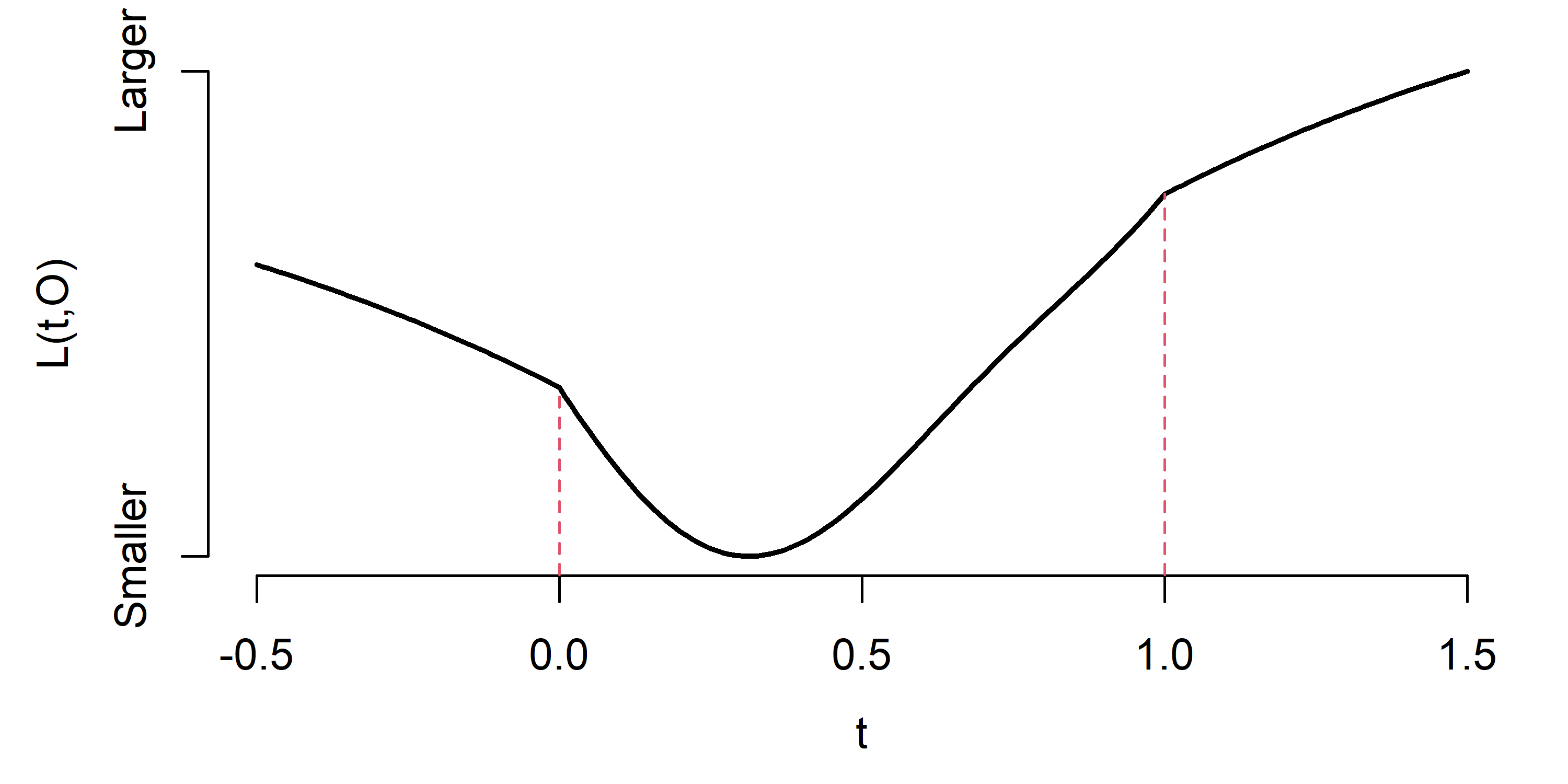
The loss function is strictly decreasing over and increasing over . Critically, the loss function is equal to in (9b) when , and it consists of two key parts: the function and the binomial coefficients with the linear term . The function replaces the outcome regression in (6) and is based on the influence function of the doubly robust estimator of the overall causal effect under partial interference (Liu et al. 2019; Park and Kang 2022; Qu et al. 2022). If desired, other functions based on the influence functions for the inverse probability-weighted (IPW) estimator or the outcome regression estimator are possible. The term with is the integral of the term with threshold in equation (6); see Section A.6 of the Supplementary Material for details. More importantly, the expected loss function (i.e., risk function) achieves its minimum when in the loss function is equal to the MRTP. The following lemma formalizes the connection between the loss function and the MRTP as follows.
Lemma 3.1 (Risk Minimization Property of the MRTP).
Hereafter, we suppress the subscript for notational brevity, and the results in subsequent sections apply to the MRTPs under both potential outcomes in (4) and (5).
Methodologically, Lemma 3.1 provides a direct approach to estimate by minimizing the risk function and this connection to risk minimization allows investigators to use a variety of methods in empirical risk minimization with the proposed loss function . As a concrete example, consider a support vector machine (SVM) estimator of using a Gaussian kernel with bandwidth . Let denote the corresponding reproducing kernel Hilbert space (RKHS). Of note, a Gaussian kernel implicitly implies that the domain has a unified dimension for all ; see Section 3.3 for further discussions. If a Gaussian kernel is not appropriate, other kernel functions that are symmetric, continuous, and positive definite can be used. The representer theorem (Kimeldorf and Wahba 1970; Schölkopf et al. 2001) states that the estimated policy can be written as where and solve
| (10) |
Here, is a seminorm of in , is a regularization parameter, , for , and . Note that the optimization problem in (10) is nonconvex, but this particular nonconvex function can be efficiently solved; see Section A.8 of the Supplementary Material for details. Finally, we winsorize the estimated policy from (10) to satisfy the support restriction on , i.e., where . Investigators can then use the winsorized policy as an estimator of the MRTP.
We conclude with some remarks about the direct approach. First, while there are theoretically optimal values of the tuning parameters and for SVMs (see Theorem 3.1 below), in practice, cross-validation is used to choose them where one starts with a grid of values for and finds the value that minimizes the cross-validated empirical risk (Steinwart and Christmann 2008; Hastie et al. 2009). Our empirical analysis also uses cross-validation to choose and Section A.9 of the Supplementary Material lays out the computational details. In general, the tuning parameter controls the bandwidth of the SVM kernel whereas the tuning parameter regularizes the SVM coefficients in (10). Second, investigators can choose function spaces other than the RKHS. For instance, if an investigator prefers a simple, linear MRTP, the investigator can replace the RKHS with a space of linear functions, i.e., , and minimize with respect to the new function space. While the estimated policy may be more interpretable under a linear space, it may have a higher excess risk bound than the policy estimated under RKHS if the true policy is not well-approximated by the space of linear functions; in fact, in this case, the excess risk bound will be bounded away from even though the number of blocks grows to infinity. Third, the difference of convex functions (DC) algorithm (An and Tao 1997) can be used to efficiently solve (10) and the computational details are in Section A.8 of the Supplementary Materials. Fourth, unlike Chen et al. 2022, which used a surrogate loss to obtain an approximation of the target loss function, our approach directly uses the target loss function in (9b) and does not require a surrogate loss function.
3.3 Estimating the Nuisance Functions
Under partial interference, some care must be exercised when estimating the two nuisance functions, the outcome regression and the propensity score. For example, for the outcome regression , naively using some popular nonparametric (or parametric) regression methods where is the dependent variable and are the independent variables will often be infeasible because the dimension of varies for each study unit and block . Thankfully, this issue is not new in modern machine learning and we briefly review some common solutions. Also, following a recent trend in causal inference using machine learning methods (e.g., Chernozhukov et al. 2018), our theoretical results are agnostic to specific estimators of the nuisance functions so long as they are estimated consistently; see Section 3.4.
We start with estimating the outcome regression . In data-rich environments where is large and is estimated using overparametrized neural networks, a common trick is to pad the vector with zeros so that all the independent variables have identical length across blocks (Goodfellow et al. 2016, Chapter 10). Alternatively, in data-scarce environments where is small to moderate or the investigator prefers simpler, nonparametric methods, it is common to modify the original to have a common dimension and then use “classic” nonparametric regression estimators, such as the Nadaraya-Watson kernel regression estimator (Nadaraya 1964; Watson 1964). Some common ways of modifying in the literature include (a) taking a random subsample of a fixed number of households from each block, (b) using covariates from the “average” or the “extreme” households, such as where and are the collection of maximum and minimum values, respectively, or (c) generating a -dimensional, low-rank summary of such as the cluster-level average . Investigators can also use an ensemble of learners based on different modifications of via the super learner algorithm (van der Laan et al. 2007; Polley and van der Laan 2010); see Section A.7 of the Supplementary Material for details. Given the moderate sample size of our data, we use approach (c) to train .
We remark that estimation of is closely tied to correctly modeling the pattern of partial interference within a block. So long as the investigator uses a sufficiently flexible estimator for that can correctly model a wide variety of interference patterns in a block, the risk of the estimated policy will converge to that of the true policy; see Theorem 3.1. In the off-chance that the investigator has a priori knowledge about the interference pattern, incorporating this knowledge into estimating can improve the finite-sample performance of the estimated policy.
For the propensity score , we suggest nonparametric and semiparametric approaches. The nonparametric approach is similar to fitting the outcome regression model where we use as the dependent variable and as the independent variable inside the super learner algorithm to estimate the propensity score . Then, we use the estimated propensity score to obtain an estimated as follows:
Implicitly, the estimator assumes that the propensity score can be decomposed into a product of individual propensity scores . If this assumption is implausible or is numerically unstable due to the product term, an alternative approach is to use a semiparametric model. Specifically, we decompose the propensity score as and estimate the first conditional probability using the same nonparametric approach discussed for estimating the outcome regression. For the second conditional probability, we bin into equi-spaced bins and consider the following ordinal regression model for parametrized by :
Here, the intercept parameters satisfy . We then estimate via the likelihood principle. The final estimator of is simply a plug-in estimator based on the estimated , i.e., . For our data example, we used the semiparametric approach as it was more numerically stable than the nonparametric approach, especially after taking measures to prevent overfitting; see the next paragraph.
We also discuss two common techniques that we used to prevent overfitting the nuisance functions. First, we randomly remove observations so that the number of study units in blocks is roughly similar to each other. This adjustment is often referred to as undersampling in multilevel studies (Fernández et al. 2018, Chapter 5.2) and the adjustment prevents a few large, outlying blocks from having a dominant effect on the estimated nuisance function. Second, for the two nuisance functions in the loss function in (9), we use cross-fitting by Chernozhukov et al. 2018 where we train the two nuisance functions and the optimal policy from two different subsamples of the data. Specifically, suppose we split the data into two folds and and let , , , be the estimated outcome regression, propensity score, and loss function, respectively, by using . We estimate the MRTP by solving the SVM in (10) where is evaluated in . Again, we take the winsorized policy to make sure the optimal policy is bounded between and , i.e., . Investigators may use either , , or the winsorized average of the two policies, i.e., , as the final estimator of the MRTP. Finally, we remark that it is common to repeat undersampling and cross-fitting multiple times and aggregate the final estimators to remove finite-sample effects from random sampling; see Section A.10 of the Supplementary Material for details.
3.4 Theoretical Properties
In this section, we study the performance of the estimated policy from the previous section. To proceed, for , let and be the convergence rates in -norm of the estimated nuisance functions. We make the following assumptions about the estimated nuisance functions and the corresponding convergence rates.
- (E1)
Overlap of : There exists a constant such that for any and .
- (E2)
Bounded : is bounded for any and .
- (E3)
Consistency of and : Let , , and be sequences of real numbers, which are as . Then, for , we have and with probability greater than .
Assumption (E1) implies that the estimated propensity score satisfies overlap and Assumption (E2) implies that the estimated outcome regression is uniformly bounded. For the WASH example, Assumption (E2) is satisfied because the outcome is binary. Assumption (E3) states that, with high probability, the estimated nuisance functions and converge to the true nuisance functions in -norm sense with rates and , respectively. We remark that similar conditions are introduced in previous works that use nonparametric methods to estimate the nuisance components; see, for example, Chernozhukov et al. 2018 under no interference with independent and identically distributed data and Sofrygin and van der Laan 2016 and Park and Kang 2022 under partial interference with independent, but not necessarily identically distributed data.
In Theorem 3.1, we characterize the excess risk of , a common metric of performance in this literature (e.g., Zhao et al. 2012; Díaz et al. 2018; Kitagawa and Tetenov 2018).
Theorem 3.1.
Suppose that Assumptions (A1)-(A5) and (E1)-(E3) hold. In addition, suppose that belongs to a Besov space where is the modulus of continuity of order and is the smoothness parameter. Then, for , and any positive numbers satisfying , we have the following excess risk bound of with probability greater than :
| (11) | ||||
Here, are constants that are independent of .
To better interpret the result, suppose the bandwidth parameter and the regularization parameter are chosen with rates and . Under these choices, the bound in (11) reduces to . The first term, , is related to the convergence rate of the SVM, which depends on the smoothness of the true MRTP . If is very smooth (i.e., with fixed ), the first term approximates the rate from Chen et al. 2022. The second term, , represents the convergence rate of the estimated nuisance functions and is a second-order bias of the nuisance function estimators. It is important to note that the absence of the first-order bias is a consequence of employing the doubly robust loss function. If both nuisance functions are estimated at rates, the second term attains rate. Finally, we remark that the excess risk bound in Chen et al. 2022 depends on a parameter associated with a surrogate loss function, which, as discussed above, is used to address the lack of smoothness in their loss function. However, in our framework, we do not employ any surrogate loss function, and as a result, our excess risk bound (11) does not depend on rates stemming from the difference between the surrogate loss function and the true loss function.
4 Simulation
We conduct a simulation study to assess the finite-sample performance of the indirect and direct approaches of estimating the MRTP. We have blocks where the block size is randomly drawn from the set and the probability of drawing an element from this set is proportional to the empirical distribution of the size of the blocks in the training data for our case study in Section 5. For unit in block , we have four pre-treatment covariates . The unit-level covariates are generated from a 3-dimensional multivariate normal distribution with , , and . The block-level covariate is generated from a standard normal distribution and is independent of . The treatment is generated from the following model: . Similar to the block size, the treatment model is designed to mimic the training data for our data application where between the simulated data and the training data are nearly identical. Lastly, the outcome is generated from a model that satisfies Assumptions (A1)-(A5); see Section A.11 of the Supplementary Material for details.
Since the estimation procedures for and are nearly identical, we focus on . For the direct approach, we unify the dimension of with , use the SVM described above, run 10-fold cross-validation for the SVM parameters, and do median-adjustment from 5 cross-fitted estimators, where each cross-fitted estimator is also median-adjusted from 3 undersampled estimators. For the indirect approach, we use two methods to estimate , a linear regression model with as regressors regularized by a Lasso penalty (Tibshirani 1996) and random forests (Breiman 2001); these methods are referred to as Lasso and RF, respectively. For the target , we vary between and , which matches the observed range in the application in Section 5. We evaluate the performance of each method on a test set consisting of 200 blocks. We repeat this entire process 50 times and, therefore, obtain 10000 MRTP estimates for each method and .
Figure 4.1 shows the squared deviations between the estimated and the true MRTPs. The direct approach shows the best performance where its squared deviation between the predicted and the true MRTPs is generally the smallest across all threshold values .

Next, we assess the methods using the following classification performance measures: accuracy, two-sided F1 score, and the Matthews correlation coefficient (MCC) (Matthews 1975); see Section A.12 of the Supplementary Material for details. For every classification performance measure, a larger value means better performance. Figure 4.2 shows the result for each method. We also plot the true MRTP for comparison. The true MRTP performs the best across the different performance measures and all thresholds , justifying that the measures are meaningful for evaluating the performance of the policies. Among the estimated policies, the direct approach generally performs well across most and the three performance measures. Combined with Figure 4.1, we would generally recommend the direct approach in terms of bias and performance measures based on classification.

5 Application: WASH Policy in Senegal
5.1 Background
We use the proposed methods to design a WASH policy for Senegal. Specifically, we use the 2014-2018 Senegal Demographic and Health Survey (DHS), which used a two-stage stratified survey design where households (i.e., the study units) are nested under census blocks. We restrict the sample to households with complete data on . For household in block , the outcome is binary where indicates that there is no child having diarrhea in the household and indicates that there is at least one child having diarrhea in the household. The treatment is binary where indicates that the household has a WASH facility, defined as having a private water source or a private flush toilet, and indicates the opposite. The covariates consist of the following nine household- and block-level characteristics: block size , the indicator of whether census block is located in an urban area, number of household members, number of children in a household, the indicator of whether both parents in a household do not have jobs, whether parents ever attended schools, mother’s age, and the average age of children.
For training data, we use the 2014-2017 DHS, which contains census blocks with households. For validation data, we use the 2018 DHS, which contains census blocks with households. Also, for the validation data, we vary the diarrhea-free target threshold from to , which is slightly above and below the average diarrhea-free incidence level of between 2014 and 2017. Then, for each , we estimate the MRTP for the overall potential outcome. For both the direct and the indirect approaches, we use the same procedures as in the simulation study except that, for the direct approach, we use 100 cross-fitted estimators with median adjustment and 10 rounds of undersampling. In Section A.13 of the Supplementary Material, we discuss how the bounded cluster size assumption and Assumptions (A1)-(A5) are plausible in the Senegal DHS.
5.2 Results
Finding 1: The direct approach is more accurate.
Figure 5.1 shows the classification performance measures. Across all performance measures, the direct approach performs better than the indirect approaches across all thresholds . Combined with the results from the simulation study, the direct approach is more accurate (i.e., smaller deviance from the true MRTP) than the other two approaches.

Figure 5.2 shows heatmaps of the estimated MRTPs at four values of the thresholds. Specifically, the heatmap shows the weighted averages of the estimated MRTPs aggregated to 45 Senegalese administrative regions where the weight is based on the number of households in a census block (i.e., ); see Section A.14 of the Supplementary Material for more details behind the heatmaps. For each , the estimated policy from the direct approach is generally more diffused than the indirect approach, implying that the direct approach generally prefers a more balanced, nationwide approach to allocating WASH facilities across Senegal compared to the indirect approach. Also, since the direct approach is more accurate than the indirect approach, the finding broadly suggests that an optimal WASH policy in Senegal is a diffuse approach where neighbors of an area with a high MRTP should also receive a relatively large amount of WASH facilities instead of a targeted, all-or-nothing approach where there are sharp discrepancies in the amount of WASH facilities allocated between two neighbors.

Finding 2: The direct approach is more resource-efficient.
Figure 5.3 shows the weighted averages of estimated MRTPs needed to achieve the target outcome level where the weight is determined by the size of the census blocks. When is greater than 0.69, which is the outcome level in the training data, the direct approach uses fewer WASH facilities than the two indirect approaches. Combined with our first finding that the direct approach is more accurate, the direct approach is more resource-efficient than the indirect approaches in terms of allocating the right regions of Senegal to achieve higher accuracy. In other words, for thresholds greater than 0.69, the direct approach uses fewer resources and is more accurate than the other methods, suggesting that the indirect approaches are targeting the wrong regions of Senegal or using more resources than necessary to achieve the target . Figure 5.2 provides some evidence of this observation where the random forest is over-allocating WASH facilities across most of Senegal, even in areas that may not need additional WASH facilities to achieve . In contrast, the direct approach generally allocates fewer resources throughout the nation while simultaneously achieving higher accuracy. Given that Senegalese policymakers would like to set higher than the current diarrhea-free incidence rate of 0.69, we would recommend the direct approach as it is not only accurate but also cost-efficient for allocating WASH facilities in Senegal.

Finding 3: Compared to current policy recommendations, the direct approach uses different characteristics to allocate WASH facilities.
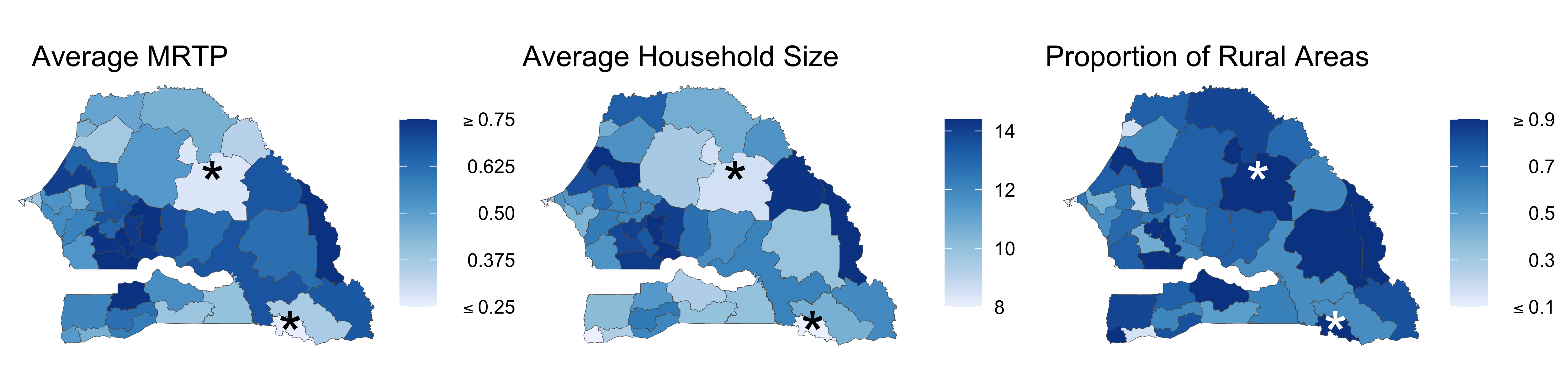
In international development, one of the prevailing advice on the allocation of WASH facilities is to target rural areas (ESARO 2019; World Bank Group 2019). Specifically, these works suggest that nations use the proportion of rural areas to allocate WASH facilities, where a large proportion of rural areas would indicate that a large number of WASH facilities is needed. However, as depicted in Figure 5.4, the direct approach suggests that this should not be the main strategy for allocating WASH facilities. Instead, the allocation policy should focus on the average household size in a census block. For example, the regions in Figure 5.4 marked with an asterisk are mostly rural areas but are associated with low MRTP estimates obtained from the direct approach. In contrast, the same regions have higher average household sizes and are associated with higher MRTP estimates. Overall, the MRTP estimate is more closely correlated with the average household size, where a census block with a large number of big households needs more WASH facilities. This positive correlation between the estimated MRTP and average household size also agrees with prior works in infectious diseases where the incidence of diarrhea is strongly correlated with household size (Yilgwan et al. 2012; Beyene and Melku 2018; Omona et al. 2020). In short, if the target outcome is to reduce the incidence of diarrhea, the direct approach suggests that household size may be a better indicator to guide policy compared to the proportion of rural areas.
Finding 4: Comparing MRTPs under different outcomes can provide insights about the mechanism of the MRTP under the primary outcome.
Using the methods developed in the paper, we can compare MRTPs from different potential outcomes by simply changing the loss functions. Importantly, these comparisons can reveal insights about the mechanism of the MRTP under the primary outcome. As an illustrative example, we compare the MRTP under the primary outcome that is discussed above (i.e., ) with the MRTP under the spillover potential outcome (i.e., ).
By Theorem 1 of VanderWeele and Tchetgen Tchetgen 2011, the difference serves as a proxy for the magnitude of the optimal policy’s direct effect on the diarrhea incidence rate. A large would indicate that the optimal policy has a large direct effect on reducing diarrhea incidence whereas a small would indicate the opposite. Also, similar to Finding 3, by comparing as a function of an observed covariate, investigators can assess the heterogeneity of the optimal policy’s direct effect.
Figure 5.5 shows one example of such heterogeneity with respect to the average number of children per household. The -axis plots the estimated by plugging in estimates of and at and the -axis plots the average number of children per household. The estimated shows a nonlinear relationship where is generally the largest when the average number of children per household is between 2.5 and 3.5. This suggests that the optimal policy’s direct effect is the largest when the average number of children per household is of moderate size. We remark that similar nonlinear trends have been observed in prior works on international development, which examined the impact of household size on diarrhea incidence or a child’s health outcome (Svanes et al. 2002; Kandala et al. 2006; Kananura 2022; Fenta et al. 2021).

6 Discussion
In this paper, we study the identification and estimation of the MRTP, a policy that assigns the smallest level of treatment to achieve a target outcome level under partial interference. We propose two approaches for estimating MRTP, a simple indirect approach where a plug-in estimator of the outcome regression model is used and a direct approach where a novel, nonparametric, doubly robust loss function that incorporates partial interference is used inside of an empirical risk minimization problem. We then use the proposed methods to estimate a WASH policy for Senegal by using the 2014-2018 Senegal DHS. We show that the direct approach is more accurate and resource-efficient than other methods. We also show a difference between our direct approach and what’s currently recommended for allocating WASH facilities in international development.
We end by discussing a few limitations of our work. First, a limitation of the MRTP in (3), , is that it does not exactly tell which study units in a block should receive treatment. This is in contrast to the optimal allocation policy in (2), , that tells which study units should be treated. However, as we discussed in Section 1, is still a valuable tool for practitioners as it provides an estimate of the minimum amount of treatment required to achieve the desired goal whereas does not provide this information. It would be interesting future work to combine the strengths of both and to obtain a more comprehensive allocation policy for international development. Second, similar to any method in causal inference with observational data, our approach relies on some assumptions, including the usual identification Assumptions (A1)-(A3) and modeling Assumptions (A4)-(A5). Policymakers should carefully evaluate the plausibility of these assumptions in the context of their research question. For example, in Section A.13 of the Supplementary Material, we assess these assumptions in our data and found no significant issues. If there is no strong evidence against these assumptions, the proposed policy can be a useful tool for policymakers.
Supplementary Material
Appendix A Additional Details of the Main Paper
A.1 Examples of Beneficial Intervention/Treatment for Most of the Population
We provide plausible examples where the intervention/treatment seems beneficial for almost all members of the population.
- •
Prior works have shown that improving household access to improved water, sanitation, and hygiene (WASH) resources are critical to reduce rates of diarrhea-related diseases (Esrey et al. 1985; Clasen et al. 2007), especially among children (Daniels et al. 1990; McMichael 2019). Additionally, there is no biological rationale that well-managed WASH facilities cause diarrhea-related diseases.
- •
Devoto et al. 2012 studied the effect of getting easier access to piped water on various kinds of outcomes such as quality and quantity of water consumed, water-related time and financial costs incurred by the household. In particular, based on the results in Table 3 and related discussions, we can deduce that getting easier access to piped water results in a substantial increase in the quantity of water for most of the population.
- •
As discussed in page 10 of Cohen and Dupas 2010, higher insecticide-treated bed nets (ITN) coverage rates would be beneficial for the population because the use of ITN in a household may have positive health externalities for neighboring households.
- •
Feikin et al. 2022 conducted a meta-analysis of studying the effect of COVID-19 vaccines against SARS-CoV-2 infection. Their work and references therein suggest that COVID-19 vaccines are beneficial for most of the population.
- •
Miguel and Kremer 2004 studied the effect of school-level deworming projects on students’ health status and academic achievements. They remarked that there were within- and across-school spillover effects, indicating that students who did not directly receive deworming treatment still benefited from those who did. Therefore, combined with the biological reasons, we can infer that deworming drugs are beneficial for most of a majority of students.
A.2 Examples of Real-world Applications Targeting a Certain Level of Outcomes
In this section, we present examples of real-world applications that target a specific level of outcomes rather than the maximum level of outcomes.
- •
High levels of protein in the urine, known as proteinuria, may be caused by diabetes, high blood pressure, autoimmune disorders, infections, and kidney diseases. Thus, for a normal adult, it is recommended to maintain the total urinary protein excretion less than 150 mg/day (Carroll and Temte 2000).
- •
HDL cholesterol is commonly referred to as “good” cholesterol because it plays a crucial role in removing harmful cholesterol from the bloodstream. As a result, maintaining high levels of HDL cholesterol is associated with a lower risk of cardiovascular disease. It is generally recommended to maintain HDL cholesterol levels above 60 mg/dL (Grundy et al. 2002).
- •
Warfarin, a blood-thinning medication, is used to increase the international normalized ratio (INR), a measure of the time for the blood to clot, and it should be prescribed to keep patients’ INR within the desired range, usually between 2 and 3, according to the recommendations from American Heart Association (January et al. 2014).
- •
Major medical associations recommend targeting proper ranges for chronic disease management measures such as hemoglobin level (male: 138-172 g/L; female: 121-151 g/L) (American Association of Clinical Endocrinologists and Others 2019).
- •
UN has established the Sustainable Development Goals in 2015 (United Nations 2016), which consists of 17 specific goals. In particular, Goal 1 is to eradicate extreme poverty for all people everywhere by 2030 and Goal 3 is to ensure healthy lives and promoting well-being at all ages. Some specifics of these goals target certain levels of outcomes of interest as follows:
- –
1.1: By 2030, eradicate extreme poverty for all people everywhere, currently measured as people living on less than $1.25 a day
- –
1.2: By 2030, reduce at least by half the proportion of men, women and children of all ages living in poverty in all its dimensions according to national definitions
- –
3.1: By 2030, reduce the global maternal mortality ratio to less than 70 per 100,000 live births
- –
3.2: By 2030, end preventable deaths of newborns and children under 5 years of age, with all countries aiming to reduce neonatal mortality to at least as low as 12 per 1,000 live births and under-5 mortality to at least as low as 25 per 1,000 live births
- –
- •
The Global Technical Strategy for malaria 2016-2030 was adopted by the World Health Assembly in May 2015 (World Health Organization 2021). It has set a target of reducing malaria incidence by 40, 75, and 90 percent by 2020, 2025, and 2030, respectively, compared with malaria incidence in 2015.
A.3 Application of Our Method to Other Real-World Examples
Motivated from the examples in Sections A.1 and A.2, we lay out some concrete examples where our approach can be used.
- •
Motivated by Cohen and Dupas 2010 and World Health Organization 2021, we can study the minimum ITN coverage necessary to meet the thresholds set by the Global Technical Strategy for malaria control Also, because an ITN is likely to reduce malaria incidence in both the household where it is installed and nearby (but not too far away) households, partial interference is a viable framework for modeling the effect of ITN installation on malaria incidence. Furthermore, there are biological reasons to believe that malaria incidence would exhibit a monotonic response to ITN coverage. Combined together, we can use our method to determine the Minimum Resource Threshold Policy (MRTP) of ITN coverage to achieve a desired malaria incidence level.
- •
Motivated by Devoto et al. 2012, we can study the minimum proportion of households with piped water that will meet or exceed the levels of existing hygiene and/or welfare indicators. For instance, as Tables 3 and 4 of Devoto et al. 2012 reported, one may use the numbers of baths and showers and the number of times a child fetched water in recent days as a basis for the hygiene and welfare indicators, respectively. Also, as suggested by Devoto et al. 2012, these indicators are likely to show monotonic response to water pipe installation. Finally, partial interference is reasonable in this context because the hygiene and welfare indicators of a household are affected by piped water in nearby (but not too far away) households. Therefore, we can use our method to determine the smallest water pipe coverage necessary to achieve the desired hygiene and/or welfare levels.
- •
We can consider a policy for allocating water, sanitation, and hygiene (WASH) in developing countries to achieve the Sustainable Development Goals 3.2 by targeting under-5 mortality being lower than 25 per 1000 live births. The context is similar to the application of the main paper except that the outcome is under-5 mortality. As before, partial interference and monotonicity are reasonable assumptions for the context, and investigators may determine the MRTPof the amount of WASH facilities that achieves the desired under-5 mortality rate.
A.4 A Graphical Illustration for the Setup
We provide a visual illustration for the setup in Figure A.1. For simplicity, we consider clusters where each cluster has study units. The black arrows from to depict the direct effect of the treatment, and the red arrows from to depict the indirect effect of the treatment. No connection between two clusters illustrate the cluster-level independence.
A.5 The (Mostly) Wrong Approach: Analysis With Aggregated, Cluster-Level Data
We briefly discuss a tempting approach based on aggregating the data at the cluster-level. This aggregation approach has been discussed in the literature (e.g., Section 2.3 of Imbens and Wooldridge 2009 and Kilpatrick and Hudgens 2021) as a simple way to deal with interference. While this approach will clearly not work for estimating MRTPs like or other MRTPs targeting spillover-specific outcomes, from a practitioner’s point of view, it is worth asking whether this approach can be used to estimate, or at least approximate, MRTPs like which combine both the direct and spillover effects of treatment in a block. Unfortunately, as we illustrate below, this aggregation approach will lead to grossly misleading estimates of except in very restrictive settings.
Formally, following the above advice from the literature, suppose an investigator attempts to bypass the problem from interference at the unit/household-level by aggregating their data at the cluster/block-level. That is, for each cluster , the investigator can consider to be the available data and use existing techniques in the optimal treatment regime literature for a continuous treatment, such as Chen et al. 2016, to obtain the minimum proportion of WASH facilities necessary to achieve a certain target . For example, given a cluster-level outcome model for the expected value of as a function of cluster-level variables and , the investigator can find the smallest where the expected outcome exceeds .
Despite its simplicity, the above analysis is only appropriate in very restrictive settings, which we illustrate with an example. Suppose the treatment assignment depends on the measured covariates, and the outcome regression is given as where are non-negative coefficients to guarantee Assumption (A5). Some algebra reveals the average potential outcome at the cluster-level is
| (12) |
If the investigator uses the aggregated, cluster-level data to estimate the MRTP, the resulting estimate will be biased because the cluster-level outcome model of given and is mis-specified. Or equivalently, there is an omitted variable bias because of the term , which roughly measures the covariance between the unit-level treatment variable and the unit-level covariate. The magnitude and the direction of the bias will depend on (a) the magnitude of treatment effect heterogeneity, as measured by and , and (b) the magnitude and the sign of the measured, unit-level confounding, as measured by the covariance of and .
More generally, if the outcome model is nonlinear, which is often the case in popular epidemiological models (e.g., Magal and Ruan 2014), no amount of modeling with aggregated, cluster-level data will completely remove this bias as the cluster-level data cannot capture both unit-level treatment heterogeneity and unit-level confounding. As a concrete example, suppose the treatment is completely randomized and there are no interactions between the covariates and the treatment, but there exists non-linear relationship between the treatment on the outcome:
| (13) |
where and are non-negative coefficients, , and is a positive integer. Roughly speaking, the model states that the household’s outcome can be affected by its peer households through a non-linear function if at least of their peers are treated; see Granovetter 1978, Watts 2002, and Kempe et al. 2003 and references therein for other types of threshold models in networks. As before, Assumptions (A4) and (A5) hold for this model and some algebra will reveal that the cluster-level outcome model will be mis-specified when using only aggregated, cluster-level data due to the non-linearity of in the household-level outcome model. Consequently, the resulting MRTP with the cluster-level data will be biased.
We provide a graphical illustration of model (13). To demonstrate, we fix the cluster size and the coefficients , and choose so that the range of the outcome regression becomes . We consider three levels for and , respectively, and we choose the threshold . Figure A.2 visually presents the differences between the MRTPs based on and the aggregated cluster-level outcome regression. We find that the differences vary between 0.07 and 0.17. The toy example suggests that estimating the MRTP based on the aggregated outcome regression may yield significantly biased estimates of in (6).

However, we mention that this simple aggregation approach may work under different assumptions. For instance, Kilpatrick and Hudgens 2021 assumed that the cluster-level potential outcome only depends on the total number of treatment implemented in a cluster, i.e., the cluster-level stratified interference. This implies that the average potential outcome at the cluster-level has a form of for some function , which can be identified as (nonparametric) regression models of on . In turn, using their -formula approach and/or the indirect approach in Section 3.1, we can get a valid estimate of . We remark that the cluster-level stratified interference assumption lacks the necessary flexibility to define . This is because it eliminates the possibility of having distinct cluster-level outcomes based on the treatment recipients, which is a critical aspect of interference.
Next, we compare the classification performance measures of the true policy of the main manuscript and the policy obtained from the aggregated cluster-level outcome regression. We consider the following simple data generating process:
The aggregated cluster-level outcome regression is given as , and the simple policy is obtained as follows:
The true policy is defined based on equation (6) of the main paper.
We generate observations from the above data generating process, and compare the three classification performance measures of and across . We use the true outcome regressions and to construct and . As a result, the discrepancies in the performance measures can be attributed to the use of the aggregated approach instead of the approach proposed of the main paper. The range of has been chosen such that the lower bound of the interval is not significantly smaller than the average outcome of . Figure A.3 graphically summarizes the result. We find that uniformly yields better classification performance measures compared to , suggesting that using the aggregated cluster-level outcome regression is suboptimal even in the simple model.

In summary, an analysis based on aggregated, cluster-level data will often lead to biased estimates of MRTP. Also, if the investigator is interested in MRTPs based on spillover-specific outcomes such as , a cluster-level analysis is simply infeasible.
A.6 Inverse Probability-Weighted and Outcome Regression-based Loss Functions
We introduce the IPW and outcome regression-based loss functions. Specifically, we can replace in (9b) of the main paper with the following functions.
A.7 Machine Learning Methods Used for the Outcome Regression Estimation
As candidate machine learning methods, we include the following methods and R packages in our super learner library: linear regression (glm), Lasso/elastic net (glmnet (Friedman et al. 2010)), spline (earth (Friedman 1991), polspline (Kooperberg 2020)), generalized additive model (gam (Hastie and Tibshirani 1986)), boosting (xgboost (Chen and Guestrin 2016), gbm (Greenwell et al. 2019)), random forest (ranger (Wright and Ziegler 2017)), and neural net (RSNNS (Bergmeir and Benítez 2012)).
A.8 Computation: Training the Support Vector Machine in (10) of the main Paper
This section presents the computational details on training the support vector machine in (10) of the main paper. The algorithm to train SVMs under this type of nonconvex function is already discussed in prior works (An and Tao 1997; Chen et al. 2016) and we present a summary of it for completeness. Also, to keep the notation clear, the discussion below assumes that the nuisance functions are known, but the identical computation algorithm is used to train the SVM when the nuisance functions are estimated.
To start off, we can decompose the loss function for the overall outcome case in equation (9) of the main paper into the difference of two convex function and , i.e., for any and where
Here, , , and is chosen as the maximum of the left derivatives of and at , i.e., and is the derivative of with respect to . Critically, the two loss functions and are convex and non-decreasing in . For the spillover outcome case, we use
Given the decomposition of the loss function into the difference of two convex functions, we use the DC algorithm (An and Tao 1997), which is an iterative algorithm, to solve the original non-convex optimization problem; see Algorithm 1 for details.
To initiate the DC algorithm, we choose the initial value as follows. First, for each , let the solution be , i.e., which can be obtained from a grid-search. In words, is an approximate of that are found by a grid-search. But, since is bounded in the unit interval, it may not be a suitable approximate of , the SVM solution before the winsorization. As a consequence, directly using to construct initial points may lead to an estimate policy shrinking to a certain value, i.e., a policy does not reflect the heterogeneity induced by . To stretch outside of the unit interval, we consider the following steps.
- (a)
Let and be
- (b)
By only using the clusters with non-0 and non-1 s, i.e., , we fit linear regression models where and are regressed on s. We choose from , i.e., 12 levels. Let are the estimated regression coefficients from th model.
- (c)
Let be the adjusted initial points which are defined as follows.
- (c-1)
If , no adjustment is required, i.e., .
- (c-2)
For clusters having , we use the largest prediction values obtained from the 13 regression models and 1, i.e.,
- (c-3)
Similarly, for clusters having , we use the smallest prediction values obtained from the 13 regression models and 0, i.e.,
- (c-1)
Second, we take and as a vector satisfying for all ; i.e., where and . Even though the kernel matrix is invertible due to the positive definiteness of the kernel function , the inverse of cannot be obtained due to the numerical singularity. Under such case, we add a tiny value to diagonal of until its inverse can be obtained. In line 1, is a subgradient of that accounts for the non-differentiability of at and .
The convex optimization in line 3 can be solved by using many standard algorithms and softwares. The iteration stops when drops below some threshold value. We remark that because the objective function in (10) of the main paper is bounded below, the algorithm will always converge in finite steps (An and Tao 1997; Chen et al. 2016).
A.9 Details of Cross-validation
We present the details on how to choose the SVM parameters and . We consider a set of candidate values for where . Without loss of generality, let the estimation data fold be and, as a consequence, observations in is used to evaluate the estimated loss function for . We further split into training and tuning sets, denoted by and , respectively, based on the number of cross-validation folds. For each candidate parameter , we estimate the direct MRTP by only using the training set and obtain the empirical risk using the tuning set . The optimal parameters are the minimizer of the average of the empirical risks across the tuning sets, i.e.
A.10 Details of Undersampling and Cross-fitting Procedures
We discuss the details on how to negate the impact of a particular realization of undersampling procedure. We randomly choose a subset of observations so that the cluster sizes are (nearly) balanced, and we repeat the undersampling for times indexed by . Let and be the estimated outcome regression and propensity score obtained from th undersample. Then, we take the median-adjusted nuisance function across estimated functions as the final estimate of the nuisance function, i.e., and .
Next, we discuss the median-adjustment of cross-fitting procedure. Once we split the data into two folds and , we obtain two directly estimated policies for where is used as the estimation data fold and is used as the evaluation data fold. Investigators may use either or as the final estimate of the MRTP, denoted by . However, we recommend to use , the winsorized policy of the average of two non-winsorized policies, for the new as the estimate of the MRTP to fully use the data. If the evaluation point is one of the points in the data, i.e., for some , we recommend using because does not depend on while depends on which may lead to an overfitted value. Second, to construct a more robust estimate of the MRTP under cross fitting, we use the recommendation in Chernozhukov et al. 2018 to our setting by taking the mean or the median of multiple MRTP estimates. Specifically, we repeat the estimation of multiple times, say times, and obtain where the sample partitions are randomly done across splits. We define the mean-MRTP estimate and the median-MRTP estimate .
A.11 Details of the Data Generating Process of the Simulation
We provide details of the data generating process of the simulation in Section 4. First, we provide the distribution of the cluster size , which is the same as the empirical distribution of in the dataset used in Section 4.
| 3 | 4 | 5 | 6 | 7 | 8 | 9 | 10 | 11 | 12 | |
| Frequency | 4 | 4 | 11 | 22 | 30 | 55 | 61 | 76 | 80 | 88 |
| Probability | 0.004 | 0.004 | 0.011 | 0.021 | 0.029 | 0.054 | 0.059 | 0.074 | 0.078 | 0.086 |
| 13 | 14 | 15 | 16 | 17 | 18 | 19 | 20 | 21 | 22 | |
| Frequency | 92 | 90 | 113 | 86 | 72 | 71 | 39 | 22 | 6 | 5 |
| Probability | 0.090 | 0.088 | 0.110 | 0.084 | 0.070 | 0.069 | 0.038 | 0.021 | 0.006 | 0.005 |
Next, in Figure A.4, we provide graphical summaries of the distributions of in the 2014-2017 Senegal DHS and the simulated datasets. The two distributions are similar to each other with the common support of .

A.12 Details of Classification Performance Measures
For an given MRTP , we define the true positives (TP), true negatives (TN), false positives (FP), and false negatives (FN) as follows:
| (14) | ||||||
Given these definitions, we use the following classification performance measures: accuracy, two-sided F1 score, and the Matthews correlation coefficient (MCC) (Matthews 1975) which are defined as follows:
The usual F1 score does not use true negatives in its score, i.e., 2TP/(2TP+FP+FN), and is sensitive to the definition of a positive label. For example, if we were to define the positive label as the opposite of the definition in equation (14), i.e., positive label if , the F1 score changes. To avoid this, we consider the two-sided F1 score, the average of the usual F1 score and the “opposite” F1 score, 2TN/(2TN+FP+FN).
A.13 Assessment of Assumptions of the Main Paper
We take a moment to discuss the plausibility of the bounded cluster size assumption and Assumptions (A1)-(A5) in the Senegal DHS.
- (Bounded )
The bounded block size assumption is plausible in the Senegal DHS because the data was collected based on a stratified sampling design where a fixed number of households were sampled from each block (1). Also, the maximum number of households among census blocks in the 2014-2017 Senegal DHS is , and the small value of (i.e., an upper bound on ) suggests that the “large , small ” asymptotic regime is a reasonable approximation for our data.
- (A1)
Assumption (A1) is plausible as long as households in different census blocks do not interact with each other. In the data, 99.15% of the census blocks are geographically far apart from each other. The average and median distances among 22,578 pairs of census blocks in the 2018 Senegal DHS are 245.04km and 230.17km, respectively; only 192 (0.85%) pairs of census blocks have distance smaller than 10km. Given this, we find that the partial interference assumption is plausible where interference likely occurs between households in the same census block and not across different census blocks.
- (A2)
To check Assumptions (A2) and (A3), we check covariate balance and overlap by using the binning approach in Hirano and Imbens 2004, Kluve et al. 2012 and Flores et al. 2012 for a continuous treatment variable. Algorithm 2 shows the details on the covariate balance assessment.
1: Divide units into four groups:
where and are chosen so that have similar sizes.2: for do3: Obtain unadjusted -statistics that compare the distribution of between and , i.e.,4: Calculate the estimated propensity score .5: Let be the deciles of .6: Let .7: Obtain -statistics that compare the distribution of between and , i.e.,8: Aggregate the -statistics obtained in Step 7 with weights from the size of , , .9: Obtain adjusted -statistics by taking the median of -statistics in Step 6 across multiple cross-fitting procedures.10: end forAlgorithm 2 Assessment of Covariate Balance We use the median of the propensity score estimates from 100 cross-fitting procedures. As a consequence, we obtain the unadjusted/adjusted -statistics in Figure A.5, which suggests covariate balance was satisfied for all cases.

Figure A.5: Covariate Balance Assessment - (A3)
Next, we assess the overlap assumption based on Algorithm 3. Again, we use the median of the propensity score estimates from 100 cross-fitting procedures.
1: Divide units into four groups:
where and are chosen so that have similar sizes.2: Calculate the median of the estimated propensity scores obtained from multiple cross-fitting procedures, i.e.,
where the conditional probability is calculated from the estimated propensity score obtained from the th cross-fitting procedure.3: Compare histograms of for and for each .Algorithm 3 Assessment of Overlap Figure A.6 shows histograms that visually assess the overlap assumption. Based on the histograms, the overlap assumption seems to be satisfied or to be not severely violated.

Figure A.6: Overlap Assessment. The numbers in brackets show the range of the estimated propensity scores for each group. Overall, all 9 observed covariates are balanced across different bins of treatment values and overlap is reasonable.
- (A4)
Assumption (A4) is plausible if the number of diarrhea-free children in a household can be reasonably approximated by a summary of peers’ WASH status. However, the assumption may fail if a few households’ presence (or absence) of WASH facilities is driving the incidence of diarrhea in the entire block, say if a few WASH-less households are located near communal water sources and they are primarily responsible for the diarrhea in the entire block. For example, if the census block has 20 households and the true response model for each household is , i.e., every household ’s outcome depends on household ’s treatment status, then and Assumption (A4) is violated because the average response of block depends on the treatment status of household . Unfortunately, the data does not contain information about the location of households to test these hypothesized violations of Assumption (A4). Instead, we visually diagnose the assumption by using a residual plot of the predicted values of the mean block-level response versus the observed block-level response. Specifically, let be the residuals where is the median of the outcome regression from 100 cross-fitting procedures. We compare the residuals across the outcome regression estimate and the regressors and check whether the residuals deviate from zero in Figure A.7. Since the dimension of varies, we use the average of , i.e., . In general, the residuals are close to zero across the regressors, implying that the outcome regression under Assumption (A4) is not severely violated. That is, while the diagnostic is not perfect, we find the predicted means do not show trends across the -axis and Assumption (A4) could be plausible, subject to inherent limitations of the diagnostic plot.

Figure A.7: Residual Plots. The -axis shows the outcome regression estimate (top left) and the regressors . The -axis shows the residuals . The red curves are smoothing lines drawn for visual guidance. The blue dashed lines show the zero residual. - (A5)
Finally, for Assumption (A5), many prior works (Esrey et al. 1985; Daniels et al. 1990; Clasen et al. 2007; Ejemot‐Nwadiaro et al. 2015; McMichael 2019) suggest that installing WASH facilities will not have a negative impact on incidence of diarrhea; however, it may have a negative effect on other, non-health outcomes. Also, when we empirically assess Assumption (A5), we find that the monotonicity assumption is rarely violated in the Senegal DHS and if violated, the deviation from monotonicity is small. Specifically, we first consider the difference between two cluster-level outcome regressions:
In particular, we focus on the variations contrasting two adjacent outcome regressions. As a consequence, there are finest variations where variations have the form , variations have the form , and variations have the form ; see the diagram below.
In the Senegal DHS, we have variations in total. Let be the estimated variation of cluster obtained from the th cross-fitting procedure, and let be the median of the variation, i.e.,
Assumption (A5) can be empirically assessed by two means. First, out of 38614 variations, we count the number of times monotonicity is violated. Second, we measure the worst-case slope of the estimated as follows. Let be the absolute value of . Thus, the sum of 38614 is the total variation of the cluster-level outcome regression. We compute the relative magnitude of the slopes that are decreasing compared to the total variation, i.e., . Overall, under the first assessment, we found that the monotonicity is violated of the time and under the second assessment, the relative magnitude of decreasing slopes is . In short, the empirical validations show that the monotonicity assumption is rarely violated in the Senegal DHS and if violated, the deviation from monotonicity is small.
A.14 Details of Figures 5.2-5.4 of the Main Paper
We additionally describe how we draw Figures 5.2-5.4 of the main paper. The reported estimated MRTPs in Figures 5.2 and 5.4 are weighted average of the estimated MRTPs in each administrative region where weights are the number of households in a census block, i.e., census block size . That is, the values represent s, which are defined as
where is the collection of census blocks in the 2018 Senegal DHS. In words, is the proportion of households in administrative area that require WASH facilities. Similarly, the average household sizes in Figure 5.4 represent
Again, is the average household wise in administrative area . The proportions of rural area in Figure 5.4 represent
Here is the proportion of the rural census blocks in administrative area . Note that , , and do not address the geographical distance between census regions in different administrative areas. But, we believe that these statistics are geographically meaningful summaries to highlight the heterogeneity across administrative areas; see Figures 1 and 2 of Houngbonon et al. 2021 for similar summary statistics aggregated at Senegalese administrative areas.
Lastly, Figure 5.3 shows the weighted average of the estimated MRTPs across all 45 administrative areas where weights are the number of households in a census block, i.e., census block size . That is, the -axis represents , which is defined as
In words, is the proportion of households in Senegal that require WASH facilities.
Appendix B Proof of Lemmas and Theorems
B.1 Useful Lemmas
Lemma B.1.
Suppose that belongs to a Besov space on with smoothness parameter , i.e., where is the modulus of continuity of order . Then, for any positive satisfying , we have the following excess risk bound of with probability not less than :
Lemma B.2.
Let be the estimated risk function where the expectation is taken with respect to while is considered as a fixed function which is clarified by denoting in the conditioning statement. Let be the collection of policies ranging over the unit interval. Under Assumption (A1)-(A5) and (E1)-(E3) of the main paper, we have with probability greater than for any where is a fixed constant, if the inverse probability-weighted loss function is used, if the outcome regression loss function is used, and if the doubly robust loss function is used.
B.2 Proof of Lemma 3.1
We only show the result about the overall outcome case because the result about the spillover outcome case is obtained from a similar manner. Let be the collection of policies ranging over the unit interval and be the winsorized function of over the unit interval, i.e.
From the definition of , we find for any and for any . As a consequence, for any policy satisfies and . This implies that , the minimizer of , must belong to .
For any function , we find and due to the constructions of and . Combining the above results, we observe the following relationship.
Thus, it suffices to show that defined in (6) of the main paper minimizes , which is represented as follows.
| (15) |
The first and second identities are trivial from the definition of and . The third identity is from the law of iterated expectation and the following algebra:
The fourth identity is from for ; we remark that any satisfying (e.g., inverse probability-weighted or outcome regression-based) can be used instead of . From the monotonicity condition (A5), it is straightforward to check that the following sets are intervals if they are non-empty:
Since and are non-overlapping intervals, we establish that and are equivalent. If and are empty, we define and , respectively. In these cases, we also establish that and are equivalent as or , respectively. We remark that, without the monotonicity condition (A5), these two sets may be disconnected sets, i.e., not intervals, and we cannot establish that and are equivalent.
B.3 Proof of Lemma B.1
We only show the result about the overall outcome case because the result about the spillover outcome case is obtained from a similar manner. The proof of B.1 is similar to that of Theorem 2 of Chen et al. 2016 which use Theorem 7.23 of Steinwart and Christmann 2008 and Theorem 2.2 and 2.3 of Eberts and Steinwart 2013. For completeness, we present a full exposition to our setting below. We first introduce Theorem 7.23 of Steinwart and Christmann 2008.
Theorem 7.23. (Oracle Inequality for SVMs Using Benign Kernels; Steinwart and Christmann 2008) Let be a loss function having non-negative value. Also, let be a separable RKHS of a measurable kernel over . Let be a distribution on . Furthermore, suppose the following conditions are satisfied.
- (C1)
For all , there exists a constant satisfying .
- (C2)
is locally Lipschitz continuous with respect to .
- (C3)
For all , we have where .
- (C4)
is satisfied for constant , , and for all .
- (C5)
For fixed , there exists constants and such that the dyadic entropy number where is the entropy number of .
We fix and a constant such that for any . Then, for all fixed and , the SVM using and satisfies
| (16) | ||||
with probability not less than , where is a constant only depending on , , , , and .
Verification of Assumption (C1): From Assumptions (A1)-(A5) and , we find that , , and are bounded and, as a consequence, in (9a) of the main paper is bounded. As a result, in (9) of the main paper is bounded as well.
Verification of Assumption (C2): We find the derivative of in (9) of the main paper is
and we find that is bounded for all except . Moreover, is continuous at and . Thus, is locally Lipschitz continuous with Lipschitz constant .
Verification of Assumption (C3): We take . It is trivial that from the form of in (9) of the main paper.
Verification of Assumption (C4): Note that . Thus, we find
We take and and the condition is satisfied.
Verification of Assumption (C5): Since we use the Gaussian kernel, we can directly use Theorem 7.34 of Steinwart and Christmann 2008 which is given below.
Theorem 7.34. (Entropy Numbers for Gaussian Kernels; Steinwart and Christmann 2008) Let be a distribution on having tail exponent . Then, for all and , there exists a constant such that
for all and .
Therefore, Assumption (C5) holds with .
As a consequence, the result in equation (16) holds with , , , , . Moreover, we find since for and this leads . Thus, we find the following result holds with probability not less than .
| (17) | ||||
The above result holds for any , so we can further bound the approximation error by choosing in a specific way which is presented in Eberts and Steinwart 2013. We first define a function as
| (18) |
for and . Since the range of is bounded between , we find . Thus, we can define by convolving with as follows (Eberts and Steinwart 2013).
Next, we introduce theorem 2.2 and 2.3 of Eberts and Steinwart 2013.
Theorem 2.2. Let us fix some . Furthermore, assume that is a distribution on that has a Lebesgue density for some . Let be such that . Then, for , , and with , we have
where is a constant only depending on and .
Theorem 2.3. Let , be the RKHS of the Gaussian kernel with parameter , and be defined by (18) for a fixed . Then we have with
Moreover, if , we have .
As a result, we obtain
| (19) | ||||
The first equality is from the construction of . The first inequality is from Theorem 2.3 of Eberts and Steinwart 2013. The second inequality is from Lipschitz continuity of . The third inequality is from Theorem 2.2 of Eberts and Steinwart 2013 with and . The last inequality holds for some constant since implies from the definition of a Besov space. Combining the results in (17) and (19), we have the following result
B.4 Proof of Lemma B.2
We only show the result about the overall outcome case because the result about the spillover outcome case is obtained from a similar manner. We find the following result for .
| (20) |
for some generic constant . The last inequality is from and bounded . Also, we find the following result for .
Finally, we find the following result for for all .
where constant is given in (B.4). Therefore, for any , we find
The first inequality is from the definition of . The second inequality is from the Jensen’s inequality. The third inequality is from the above results. The last inequality is from the definition of . Therefore, it suffices to bound for all three types of where .
First, the difference between and is
The upper bound is from the bounded outcome and Assumptions (A3) and (E1). Thus, we find the following result with probability greater than :
where .
Second, we study the difference between and which is
Therefore, we find the following result with probability greater than .
where .
Lastly, we prove the result when is chosen. From (B.4), we have
where the sign of is chosen to satisfy the inequality above. The expectation of is
The equalities are straightforward from the definition of and the law of total expectation. Since , we find
The first inequality is straightforward. The second inquality is from the Hölder’s inequality. From the last line, we find . As a result, we have the following result with probability greater than .
where .
Combining the established results, we have the following results with probability greater than .
This implies with probability greater than where , if the inverse probability-weighted loss function is used, if the outcome regression loss function is used, and if the doubly robust loss function is used.
B.5 Proof of Theorem 3.1
We only show the result related to the overall outcome case because the result related to the spillover outcome case is obtained in a similar manner. We start with defining the risk function and the MRTP associated with the estimated loss function. Let be the estimated risk function where the expectation is taken with respect to while is considered as a fixed function which is clarified by denoting in the conditioning statement. Accordingly, let be the approximated MRTP which is the minimizer of , i.e., for all . We remark that , the collection of policies ranging over the unit interval. Using as the intermediate quantities, we can establish the excess risk of .
We decompose the excess risk as follows.
In the rest of the proof, we bound terms , , and .
From Lemma B.2 of the Supplementary Material, we find the upper bound of with probability greater than :
Next, we bound . Since satisfies Assumptions (C1)-(C5) and belongs to a Besov space , Theorem B.1 can be applied. Hence, the following result is satisfied with probability greater than :
Lastly, we bound . Since is the minimizer of , we find
and this implies . Similarly, since is the minimizer of , we find
and this implies , i.e., . Combining two results, we have
From Lemma B.2 of the Supplementary Material, the right hand side of the above term is upper bounded by with probability greater than because . As a result, we find an upper bound of , which is . We remark that and are both with probability greater than . This concludes the desired result.
References
- Agence Nationale de la Statistique et de la Démographie (ANSD) and ICF (2020) Agence Nationale de la Statistique et de la Démographie (ANSD) and ICF (2020). Sénégal: Enquête Démographique et de Santé Continue (EDS-Continue 2018). Available from https://dhsprogram.com/pubs/pdf/FR367/FR367.pdf.
- American Association of Clinical Endocrinologists and Others (2019) American Association of Clinical Endocrinologists and Others (2019). Management of common comorbidities of diabetes.
- An and Tao (1997) An, L. T. H. and Tao, P. D. (1997). Solving a class of linearly constrained indefinite quadratic problems by dc algorithms. Journal of Global Optimization, 11(3):253–285.
- Aronow and Samii (2017) Aronow, P. M. and Samii, C. (2017). Estimating average causal effects under general interference, with application to a social network experiment. The Annals of Applied Statistics, 11(4):1912–1947.
- Bargagli-Stoffi et al. (2020) Bargagli-Stoffi, F. J., Tortù, C., and Forastiere, L. (2020). Heterogeneous treatment and spillover effects under clustered network interference. Preprint arXiv:2008.00707. IMT School for Advanced Studies Lucca, Lucca.
- Barkley et al. (2020) Barkley, B. G., Hudgens, M. G., Clemens, J. D., Ali, M., and Emch, M. E. (2020). Causal inference from observational studies with clustered interference, with application to a cholera vaccine study. Annals of Applied Statistics, 14(3):1432–1448.
- Benjamin-Chung et al. (2018) Benjamin-Chung, J., Amin, N., Ercumen, A., Arnold, B. F., Hubbard, A. E., Unicomb, L., Rahman, M., Luby, S. P., and Colford, John M, J. (2018). A Randomized Controlled Trial to Measure Spillover Effects of a Combined Water, Sanitation, and Handwashing Intervention in Rural Bangladesh. American Journal of Epidemiology, 187(8):1733–1744.
- Bergmeir and Benítez (2012) Bergmeir, C. and Benítez, J. M. (2012). Neural networks in R using the stuttgart neural network simulator: RSNNS. Journal of Statistical Software, 46(7):1–26.
- Beyene and Melku (2018) Beyene, S. G. and Melku, A. T. (2018). Prevalence of diarrhea and associated factors among under five years children in harena buluk woreda oromia region, southeast ethiopia, 2018. Journal of Public Health International, 1(2):1–9.
- Breiman (2001) Breiman, L. (2001). Random forests. Machine learning, 45(1):5–32.
- Carroll and Temte (2000) Carroll, M. F. and Temte, J. L. (2000). Proteinuria in adults: A diagnostic approach. American family physician, 62(6):1333–1340.
- Chakraborty and Moodie (2013) Chakraborty, B. and Moodie, E. (2013). Statistical Methods for Dynamic Treatment Regimes, volume 2. Springer, New York.
- Chen et al. (2022) Chen, G., Li, X., and Yu, M. (2022). Policy learning for optimal individualized dose intervals. In Proceedings of The 25th International Conference on Artificial Intelligence and Statistics, volume 151 of Proceedings of Machine Learning Research, pages 1671–1693.
- Chen et al. (2016) Chen, G., Zeng, D., and Kosorok, M. R. (2016). Personalized dose finding using outcome weighted learning. Journal of the American Statistical Association, 111(516):1509–1521.
- Chen and Guestrin (2016) Chen, T. and Guestrin, C. (2016). Xgboost: A scalable tree boosting system. In Proceedings of the 22nd ACM SIGKDD International Conference on Knowledge Discovery and Data Mining, KDD ’16, page 785–794.
- Chernozhukov et al. (2018) Chernozhukov, V., Chetverikov, D., Demirer, M., Duflo, E., Hansen, C., Newey, W., and Robins, J. (2018). Double/debiased machine learning for treatment and structural parameters. The Econometrics Journal, 21(1):C1–C68.
- Clasen et al. (2007) Clasen, T., Schmidt, W.-P., Rabie, T., Roberts, I., and Cairncross, S. (2007). Interventions to improve water quality for preventing diarrhoea: systematic review and meta-analysis. BMJ, 334(7597):782.
- Cohen and Dupas (2010) Cohen, J. and Dupas, P. (2010). Free Distribution or Cost-Sharing? Evidence from a Randomized Malaria Prevention Experiment*. The Quarterly Journal of Economics, 125(1):1–45.
- Cox (1958) Cox, D. R. (1958). Planning of Experiments. Wiley, New York.
- Daniels et al. (1990) Daniels, D., Cousens, S. N., Makoae, L., and Feachem, R. (1990). A case-control study of the impact of improved sanitation on diarrhoea morbidity in lesotho. Bulletin of the World Health Organization, 68(4):455.
- Deliu and Chakraborty (2022) Deliu, N. and Chakraborty, B. (2022). Dynamic treatment regimes for optimizing healthcare. In The Elements of Joint Learning and Optimization in Operations Management, pages 391–444. Springer.
- Devoto et al. (2012) Devoto, F., Duflo, E., Dupas, P., Parienté, W., and Pons, V. (2012). Happiness on tap: Piped water adoption in urban morocco. American Economic Journal: Economic Policy, 4(4):68–99.
- Díaz et al. (2018) Díaz, I., Savenkov, O., and Ballman, K. (2018). Targeted learning ensembles for optimal individualized treatment rules with time-to-event outcomes. Biometrika, 105(3):723–738.
- Eberts and Steinwart (2013) Eberts, M. and Steinwart, I. (2013). Optimal regression rates for svms using gaussian kernels. Electronic Journal of Statistics, 7:1–42.
- Ejemot‐Nwadiaro et al. (2015) Ejemot‐Nwadiaro, R. I., Ehiri, J. E., Arikpo, D., Meremikwu, M. M., and Critchley, J. A. (2015). Hand washing promotion for preventing diarrhoea. Cochrane Database of Systematic Reviews, (9).
- ESARO (2019) ESARO (2019). Guidelines for developing a wash budget brief. Social Policy and Research Section UNICEF Regional Office for Eastern and Southern Africa (ESARO), Available from https://www.unicef.org/esa/documents/budget-brief-guidelines.
- Esrey et al. (1985) Esrey, S. A., Feachem, R. G., and Hughes, J. M. (1985). Interventions for the control of diarrhoeal diseases among young children: improving water supplies and excreta disposal facilities. Bulletin of the World Health organization, 63(4):757.
- Feikin et al. (2022) Feikin, D. R., Higdon, M. M., Abu-Raddad, L. J., Andrews, N., Araos, R., Goldberg, Y., Groome, M. J., Huppert, A., O’Brien, K. L., Smith, P. G., Wilder-Smith, A., Zeger, S., Deloria Knoll, M., and Patel, M. K. (2022). Duration of effectiveness of vaccines against SARS-CoV-2 infection and COVID-19 disease: results of a systematic review and meta-regression. The Lancet, 399(10328):924–944.
- Fenta et al. (2021) Fenta, H. M., Zewotir, T., and Muluneh, E. K. (2021). Spatial data analysis of malnutrition among children under-five years in ethiopia. BMC Medical Research Methodology, 21(1):232.
- Fernández et al. (2018) Fernández, A., García, S., Galar, M., Prati, R. C., Krawczyk, B., and Herrera, F. (2018). Learning from Imbalanced Data Sets. Springer, Berlin.
- Flores et al. (2012) Flores, C. A., Flores-Lagunes, A., Gonzalez, A., and Neumann, T. C. (2012). Estimating the Effects of Length of Exposure to Instruction in a Training Program: The Case of Job Corps. The Review of Economics and Statistics, 94(1):153–171.
- Friedman et al. (2010) Friedman, J., Hastie, T., and Tibshirani, R. (2010). Regularization paths for generalized linear models via coordinate descent. Journal of Statistical Software, 33(1):1–22.
- Friedman (1991) Friedman, J. H. (1991). Multivariate adaptive regression splines. The Annals of Statistics, 19(1):1 – 67.
- Goodfellow et al. (2016) Goodfellow, I., Bengio, Y., and Courville, A. (2016). Deep Learning. MIT Press.
- Granovetter (1978) Granovetter, M. (1978). Threshold models of collective behavior. American Journal of Sociology, 83(6):1420–1443.
- Greenwell et al. (2019) Greenwell, B., Boehmke, B., Cunningham, J., and Developers, G. (2019). gbm: Generalized Boosted Regression Models. R package version 2.1.5.
- Grundy et al. (2002) Grundy, S. M., Becker, D., Clark, L. T., Cooper, R. S., Denke, M. A., Howard, J., Hunninghake, D. B., Illingworth, D. R., Luepker, R. V., McBride, P., et al. (2002). Detection, evaluation, and treatment of high blood cholesterol in adults (adult treatment panel iii). Circulation, 106(25):3143–3421.
- Halloran (2019) Halloran, M. E. (2019). Analysis of vaccine studies and causal inference. In Handbook of Infectious Disease Data Analysis, pages 129–156. Chapman and Hall/CRC, Boca Raton.
- Hastie and Tibshirani (1986) Hastie, T. and Tibshirani, R. (1986). Generalized additive models. Statistical Science, 1(3):297 – 310.
- Hastie et al. (2009) Hastie, T., Tibshirani, R., and Friedman, J. (2009). The Elements of Statistical Learning: Data Mining, Inference and Prediction. Springer, New York, 2 edition.
- Hernán and Robins (2020) Hernán, M. A. and Robins, J. M. (2020). Causal Inference: What If. Chapman & Hall/CRC, Boca Raton.
- Hirano and Imbens (2004) Hirano, K. and Imbens, G. W. (2004). The propensity score with continuous treatments. pages 73–84. John Wiley, New York.
- Houngbonon et al. (2021) Houngbonon, G. V., Le Quentrec, E., and Rubrichi, S. (2021). Access to electricity and digital inclusion: evidence from mobile call detail records. Humanities and Social Sciences Communications, 8(1):170.
- Hudgens and Halloran (2008) Hudgens, M. G. and Halloran, M. E. (2008). Toward causal inference with interference. Journal of the American Statistical Association, 103(482):832–842.
- Imbens and Wooldridge (2009) Imbens, G. W. and Wooldridge, J. M. (2009). Recent developments in the econometrics of program evaluation. Journal of Economic Literature, 47(1):5–86.
- January et al. (2014) January, C. T., Wann, L. S., Alpert, J. S., Calkins, H., Cigarroa, J. E., Cleveland, J. C., Conti, J. B., Ellinor, P. T., Ezekowitz, M. D., Field, M. E., et al. (2014). 2014 AHA/ACC/HRS guideline for the management of patients with atrial fibrillation: ”A” report of the American College of Cardiology/American Heart Association Task Force on Practice Guidelines and the Heart Rhythm Society. Journal of the American College of Cardiology, 64(21):e1–e76.
- Jiang et al. (2022) Jiang, C., Wallace, M. P., and Thompson, M. E. (2022). Dynamic treatment regimes with interference. Canadian Journal of Statistics.
- Kananura (2022) Kananura, R. M. (2022). Machine learning predictive modelling for identification of predictors of acute respiratory infection and diarrhoea in uganda’s rural and urban settings. PLOS Global Public Health, 2(5):1–30.
- Kandala et al. (2006) Kandala, N.-B., Magadi, M. A., and Madise, N. J. (2006). An investigation of district spatial variations of childhood diarrhoea and fever morbidity in malawi. Social Science & Medicine, 62(5):1138–1152.
- Kempe et al. (2003) Kempe, D., Kleinberg, J., and Tardos, E. (2003). Maximizing the spread of influence through a social network. In Proceedings of the Ninth ACM SIGKDD International Conference on Knowledge Discovery and Data Mining, KDD ’03, page 137–146, New York, NY, USA. Association for Computing Machinery.
- Kilpatrick and Hudgens (2021) Kilpatrick, K. W. and Hudgens, M. G. (2021). G-Formula for observational studies with partial interference, with application to bed net use on malaria. Preprint arXiv:2102.01155.
- Kimeldorf and Wahba (1970) Kimeldorf, G. S. and Wahba, G. (1970). A correspondence between bayesian estimation on stochastic processes and smoothing by splines. Annals of Mathematical Statistics, 41(2):495–502.
- Kitagawa and Tetenov (2018) Kitagawa, T. and Tetenov, A. (2018). Who should be treated? Empirical welfare maximization methods for treatment choice. Econometrica, 86(2):591–616.
- Kluve et al. (2012) Kluve, J., Schneider, H., Uhlendorff, A., and Zhao, Z. (2012). Evaluating continuous training programmes by using the generalized propensity score. Journal of the Royal Statistical Society: Series A (Statistics in Society), 175(2):587–617.
- Kooperberg (2020) Kooperberg, C. (2020). polspline: Polynomial Spline Routines. R package version 1.1.19.
- Kosorok and Moodie (2015) Kosorok, M. R. and Moodie, E. E. M. (2015). Adaptive Treatment Strategies in Practice: Planning Trials and Analyzing Data for Personalized Medicine. ASA-SIAM Series on Statistics and Applied Probability, Philadelphia.
- Laber et al. (2018) Laber, E. B., Meyer, N. J., Reich, B. J., Pacifici, K., Collazo, J. A., and Drake, J. M. (2018). Optimal Treatment Allocations in Space and Time for On-Line Control of an Emerging Infectious Disease. Journal of the Royal Statistical Society Series C: Applied Statistics, 67(4):743–789.
- Liu and Hudgens (2014) Liu, L. and Hudgens, M. G. (2014). Large sample randomization inference of causal effects in the presence of interference. Journal of the American Statistical Association, 109(505):288–301.
- Liu et al. (2016) Liu, L., Hudgens, M. G., and Becker-Dreps, S. (2016). On inverse probability-weighted estimators in the presence of interference. Biometrika, 103(4):829–842.
- Liu et al. (2019) Liu, L., Hudgens, M. G., Saul, B., Clemens, J. D., Ali, M., and Emch, M. E. (2019). Doubly robust estimation in observational studies with partial interference. Stat, 8(1):e214.
- Magal and Ruan (2014) Magal, P. and Ruan, S. (2014). Susceptible-infectious-recovered models revisited: From the individual level to the population level. Mathematical Biosciences, 250:26–40.
- Matthews (1975) Matthews, B. (1975). Comparison of the predicted and observed secondary structure of t4 phage lysozyme. Biochimica et Biophysica Acta (BBA) - Protein Structure, 405(2):442–451.
- McMichael (2019) McMichael, C. (2019). Water, sanitation and hygiene (wash) in schools in low-income countries: A review of evidence of impact. International Journal of Environmental Research and Public Health, 16(3).
- Miguel and Kremer (2004) Miguel, E. and Kremer, M. (2004). Worms: Identifying impacts on education and health in the presence of treatment externalities. Econometrica, 72(1):159–217.
- Nadaraya (1964) Nadaraya, E. A. (1964). On estimating regression. Theory of Probability & Its Applications, 9(1):141–142.
- Omona et al. (2020) Omona, S., Malinga, G. M., Opoke, R., Openy, G., and Opiro, R. (2020). Prevalence of diarrhoea and associated risk factors among children under five years old in Pader District, northern Uganda. BMC Infectious Diseases, 20(1):37.
- Park and Kang (2022) Park, C. and Kang, H. (2022). Efficient semiparametric estimation of network treatment effects under partial interference. Biometrika, 109(4):1015–1031.
- Perez-Heydrich et al. (2014) Perez-Heydrich, C., Hudgens, M. G., Halloran, M. E., Clemens, J. D., Ali, M., and Emch, M. E. (2014). Assessing effects of cholera vaccination in the presence of interference. Biometrics, 70(3):731–741.
- Polley and van der Laan (2010) Polley, E. C. and van der Laan, M. J. (2010). Super learner in prediction. Technical report 200. Division of Biostatistics, Working Paper Series.
- Qu et al. (2022) Qu, Z., Xiong, R., Liu, J., and Imbens, G. (2022). Efficient treatment effect estimation in observational studies under heterogeneous partial interference. Preprint arXiv:2107.12420.
- Ren et al. (2022) Ren, J., Liu, M., Liu, Y., and Liu, J. (2022). Optimal resource allocation with spatiotemporal transmission discovery for effective disease control. Infectious Diseases of Poverty, 11(1):34.
- Richter et al. (1999) Richter, A., Brandeau, M. L., and Owens, D. K. (1999). An analysis of optimal resource allocation for prevention of infection with human immunodeficiency virus (hiv) in injection drug users and non-users. Medical Decision Making, 19(2):167–179.
- Rubin (1986) Rubin, D. B. (1986). Which ifs have causal answers? (comment on “statistics and causal inference” by P. W. Holland). Journal of the American Statistical Association, 81(396):961–962.
- Schölkopf et al. (2001) Schölkopf, B., Herbrich, R., and Smola, A. J. (2001). A generalized representer theorem. In Helmbold, D. and Williamson, B., editors, Computational Learning Theory, pages 416–426. Springer, Berlin, Heidelberg.
- Sobel (2006) Sobel, M. E. (2006). What do randomized studies of housing mobility demonstrate? Journal of the American Statistical Association, 101(476):1398–1407.
- Sofrygin and van der Laan (2016) Sofrygin, O. and van der Laan, M. J. (2016). Semi-parametric estimation and inference for the mean outcome of the single time-point intervention in a causally connected population. Journal of Causal Inference, 5(1).
- Steinwart and Christmann (2008) Steinwart, I. and Christmann, A. (2008). Support vector machines. Springer-Verlag, New York.
- Su et al. (2019) Su, L., Lu, W., and Song, R. (2019). Modelling and estimation for optimal treatment decision with interference. Stat, 8(1):e219.
- Svanes et al. (2002) Svanes, C., Jarvis, D., Chinn, S., Omenaas, E., Gulsvik, A., and Burney, P. (2002). Early exposure to children in family and day care as related to adult asthma and hay fever: results from the european community respiratory health survey. Thorax, 57(11):945–950.
- Tchetgen Tchetgen and VanderWeele (2012) Tchetgen Tchetgen, E. J. and VanderWeele, T. J. (2012). On causal inference in the presence of interference. Statistical Methods in Medical Research, 21(1):55–75.
- Tibshirani (1996) Tibshirani, R. (1996). Regression shrinkage and selection via the lasso. Journal of the Royal Statistical Society. Series B (Methodological), 58(1):267–288.
- Tsiatis et al. (2019) Tsiatis, A. A., Davidian, M., Holloway, S. T., and Laber, E. B. (2019). Dynamic Treatment Regimes: Statistical Methods for Precision Medicine. CRC press.
- United Nations (2016) United Nations (2016). Transforming our world: The 2030 agenda for sustainable development. Available at https://stg-wedocs.unep.org/bitstream/handle/20.500.11822/11125/unepswiosm1inf7sdg.pdf?sequence=1.
- van der Laan (2014) van der Laan, M. J. (2014). Causal inference for a population of causally connected units. Journal of Causal Inference, 2(1):13–74.
- van der Laan et al. (2007) van der Laan, M. J., Polley, E. C., and Hubbard, A. E. (2007). Super learner. Statistical Applications in Genetics and Molecular Biology, 6(1).
- VanderWeele and Tchetgen Tchetgen (2011) VanderWeele, T. J. and Tchetgen Tchetgen, E. J. (2011). Effect partitioning under interference in two-stage randomized vaccine trials. Statistics & Probability Letters, 81(7):861–869.
- Viviano (2021) Viviano, D. (2021). Policy targeting under network interference. Preprint arXiv:1906.10258. Department of Economics, University of California-San Diego.
- Watson (1964) Watson, G. S. (1964). Smooth regression analysis. Sankhyā, Series A, pages 359–372.
- Watts (2002) Watts, D. J. (2002). A simple model of global cascades on random networks. Proceedings of the National Academy of Sciences, 99(9):5766–5771.
- World Bank Group (2019) World Bank Group (2019). Delivering rural sanitation programs at scale, with equity and sustainability: A call to action. Available from https://blogs.worldbank.org/water/why-rural-sanitation-matters.
- World Health Organization (2013) World Health Organization (2013). Ending preventable child deaths from pneumonia and diarrhoea by 2025: the integrated global action plan for pneumonia and diarrhoea (GAPPD).
- World Health Organization (2021) World Health Organization (2021). Global technical strategy for malaria 2016–2030, 2021 update. Geneva: World Health Organization, pages 1–40.
- Wright and Ziegler (2017) Wright, M. N. and Ziegler, A. (2017). ranger: A fast implementation of random forests for high dimensional data in C++ and R. Journal of Statistical Software, 77(1):1–17.
- Yilgwan et al. (2012) Yilgwan, C. S., Okolo, S., et al. (2012). Prevalence of diarrhea disease and risk factors in jos university teaching hospital, nigeria. Annals of African medicine, 11(4):217.
- Zhao et al. (2012) Zhao, Y., Zeng, D., Rush, A. J., and Kosorok, M. R. (2012). Estimating individualized treatment rules using outcome weighted learning. Journal of the American Statistical Association, 107(499):1106–1118.