BLUE: A 3D Dynamic Bipedal Robot
Abstract
The objective of this work is to design a mechatronic bipedal robot with mobility in 3D environments. The designed robot has a total of six actuated degrees of freedom (DoF), each leg has two DoF located at the hip: one for abduction/adduction and another for thigh flexion/extension, and a third DoF at the knee for the shin flexion/extension. This robot is designed with point-feet legs to achieve a dynamic underactuated walking. Each actuator in the robot includes a DC gear motor, an encoder for position measurement, a flexible joint to form a series flexible actuator, and a feedback controller to ensure trajectory tracking. In order to reduce the total mass of the robot, the shin is designed using topology optimization. The resulting design is fabricated using 3D printed parts, which allows to get a robot’s prototype to validate the selection of actuators. The preliminary experiments confirm the robot’s ability to maintain a stand-up position and let us drawn future works in dynamic control and trajectory generation for periodic stable walking.
Index Terms:
Bipedal robot, dynamic walking, , series flexible actuator, Topological optimizationI Introduction
At the end of the 20th century, Quiang et al., developed a method to plan a biped gait of a bipedal robot dividing the task into a foot and hip trajectories [1]. This was carried out through a gait pattern generator, which used constraints generated with a third order spline interpolation. These constraints were imposed on the foot and hip trajectories. Later on, at the beginning of the 21st century, Gienger et al., designed an anthropomorphic bipedal robot to achieve a dynamic three-dimensional gait using weight reduction methods [2]. Weng specifically focused on modeling the three-dimensional dynamics of a humanoid robot, known as TEO, using Webots as a simulator, where, basically, its purpose was to show the robot’s movement in a virtual environment to perform predefined tasks [3]. For its development, it started with the creation of eight nodes, which contemplated the number of joints that are connected, then they analyzed the degrees of freedom existing in the mechanism. Using an equivalent approach, Park et al., [4] identify the dynamic model of a bipedal robot, known as MABEL, which includes a set of differential cables and integrates a torso assembled with two legs, in which each one functions as a monopod with a transmission mechanism implemented with the differential cable. An evolution of MABEL was developed with the 3D bipedal robot ATRIAS [5].
On the other hand, [6] A control strategy is proposed for its application in the stable gait of bipedal robots with random disturbances present in the trajectory. To do this, a trajectory generator is applied that defines the parameters to be followed by each of the actuators present in the leg, mainly for the change of leg during the walk. For the implementation, use is made of a generalized multivariable PI controller without switching, which is responsible for rejecting the disturbances present in the environment to which the robot is directed. Some time later, in [7], the development of control techniques in continuous and discrete time continued with a focus on following the trajectories for each joint and where the impact generated on the leg by the change of support in the walk was taken into account.
In [8] the most common failure with respect to the dynamic gait of bipedal robots is evidenced, and it is that they highlight that the limitations in performance are mainly due to the limitations caused by the mechanical design since to date most were built with complex mechanisms that hindered the transmission of kinetic energy and the focus on rigid transmissions of motion. That is why the use of springs as an improvement for the kinematic design of the legs is proposed as a solution, achieving a better energy storage, and a high mechanical power transmission. In the same vein, the ATRIAS 2.1 robot is developed in search of efficiency in the transfer of energy, speed and above all robustness with respect to the terrain of the walk, which seeks not to depend on the vision of the robot. Once raised, as indicated in [9], the legs are designed to be light, specifically less than 5 percent of the total mass, which are actuated by series-connected spring actuators. Like its predecessors, the ATRIAS 2.1 robot makes use of the inverted pendulum mechanism.
A more recent design is the one presented in [10], where, at MIT, they made a Mini Cheetah where one of its key peculiarities is the redesign of the actuators and joints since the components are easy to replace due to the size and simpler. mechanics. In the document they focus on the design and manufacture of Mini Cheetah actuators, which correspond to a new generation of these. Modular actuators have the particularity that they have a brushless motor and the gearbox is stationary, this differs from the original because the motor was in series with the actuator.
II Design requirements
The design requirements of the BLUE bipedal robot are established, which were to generate a structure from the use of independent mechanisms that offered the option of being modular with an operating torque that did not exceed 2 Nm. In addition to this, the desired average angular velocity for the mobility of each section was taken into account, where a value of 70 RPM was validated at the output of each of the actuators.
III Design of bipedal robot BLUE
The development of the BLUE bipedal robot is based on the use of six (6) mechanical actuators, each strategically located to simulate the three (3) degrees of freedom present in the proposed leg, these have a DC motor with a gearbox in such a way that after the implementation of some logic module such as H bridges it is possible to control the direction of rotation of each body. The representation is evidenced in the Figure 1

The structure of the mechanical actuator is based on the principle of reduction by use of synchronous belts where the first pulley, assembled to the motor shaft, transmits the movement by means of a 70XL reference toothed belt to a larger diameter pulley coupled to a transmission shaft, which at in turn, it transmits the energy through a 116XL reference toothed belt, with which in the end a reduction was obtained at the actuator output, in addition, it is worth highlighting one of the main strengths of the actuator design, which is to be a modular device.
| Synchronouss Belts Powergrip | ||||
| Description | Pitch length | Number of | Step | Belt height |
| [mm] | teeth | [mm] | [mm] | |
| 70XL | 177.80 | 35 | 5.08 | 2.3 |
| 116XL | 294.64 | 58 | 5.08 | 2.3 |
From the belt transmission system generated with the help of the Inventor software, the calculation of the angular velocities and the torques present along the axes was carried out and evidence was left in the Table II. Which was completed as of Equation 1, Equation 2, Equation 3 and Equation 4
| (1) |
| (2) |
| (3) |
| (4) |
where:
Pitch diameter’s
Output angular velocity
axle angular velocity
Output torque
Axle torque
| Angular velocity [rpm] | Torque [Nm] | ||||
|---|---|---|---|---|---|
| 29 | 11.48 | 21.75 | 2.63 | 6.66 | 3.51 |
| 37 | 14.57 | 27.75 | 2.06 | 5.24 | 2.75 |
| 45 | 17.72 | 33.75 | 1.69 | 4.31 | 2.26 |
| 51 | 20.08 | 38.25 | 1.49 | 3.80 | 1.99 |
| 67 | 26.38 | 50.25 | 1.14 | 2.89 | 1.52 |
| 74 | 29.14 | 55.5 | 1.03 | 2.62 | 1.37 |
| 81 | 31.89 | 60.75 | 0.94 | 2.40 | 1.26 |
| 98 | 38.58 | 73.5 | 0.78 | 1.98 | 1.04 |
| 107 | 42.13 | 80.25 | 0.71 | 1.81 | 0.95 |
| 121 | 47.64 | 90.75 | 0.63 | 1.60 | 0.84 |
- •
Transmission axis design

Fig. 2: Transmission shaft The transmission shaft was machined in silver steel as a greater resistance to the stress that would arise in the use of the composite belt system was required. For the stress analysis, the ASME - elliptical theory mentioned in Equation 5 and transformed according to the forces present in each section was used.
(5) After the stress analysis, the minimum diameters specified in the design were validated, which were , , and this because they were capable of withstand torques calculated in Table II
- •
Internal axis design
In the same way, for the design of the internal axis evidenced in 3(a), the ASME - elliptical theory mentioned in Equation 5 was taken into account, however, for this case it was verified that in none of the different sections along the axis the calculated torque was exceeded.
(6) It was determined that along the axis, the lowest torque capable of withstanding was value that when compared with Table II guarantees that at no time the axis would fail due to stress cutting. In this way, the design of the shaft was validated, which should be noted that it was made up of pieces printed in PLA material with a 90-percent filling and rigidly joined.
- •
Base design

(a) 
(b) Fig. 3: a) Internal shaft. b) Actuator base The base of the mechanical actuator was one of the principal pieces to take into account within the design due to its great effort to contain the system made up of belts and the need for a structure capable of protecting the position of the motor and the eventual vibrations that would come to throughout the experimental tests. The critical points of the structure evidenced in 3(b) were analyzed, and the maximum force capable of withstanding was determined for each case.
(7) For each case, the corresponding efforts were replaced together in Equation 7 with the known data of the torques exerted in each of the sections, where it was determined that the critical zone in the event of possible failure was the motor support with a force it is evidenced in Equation 8, however, as it is not a more demanding part, it was validated and implemented in the final design.
(8) - •
Thigh Design

Fig. 4: Femur of bipedal robot BLUE The femur of the BLUE robot was designed from the requirement of the interconnection between the actuator located in the thigh and the actuator of the knee, where, in addition to maintaining the limit in the standard measures proposed for the robot, it was defined as a restriction the internal location of the actuators, which also allowed the correct distribution of the electrical wiring along the link, as observed in Figure 4
(9) Because the femur is a piece subjected to bending and tension, the stress analysis was carried out to determine the maximum force capable of withstanding, for which the data provided by Inventor were taken and to have a range of action in the tensile force, the which was approximately as evidenced in Equation 10
(10) It was determined that the change in the lower section of the piece was the most prone to failure, although with a fairly high operating range, since a maximum bending force of was selected. To reduce risks in the experimental tests, it was proposed to make use of highlighted joints in such a way as to reduce the existing stress concentrators.
- •
Shin Design
The shin design considers a mass distribution such that the robot’s dynamic model resembles an inverted pendulum model, which allows to reduce the order of the system and carry out simpler stability analysis than with the full order model. To define the shin shape a generative design is performed using topological optimization, the necessary border parameters for the operation were defined, among which it is necessary to fix the front face of the piece together with its holes with a preservation diameter of . Likewise, the normal tension force generated in the lower hole corresponding to is used, which is a data higher than the total weight of the robot in order to maintain an operating range in the physical restriction. The result is evidenced in Figure 5

Fig. 5: Shin of bipedal robot BLUE by topological optimization
Because each of the pieces with the highest critically index in the initial prototype was validated, the preliminary assembly of the BLUE bipedal robot was carried out as evidenced in Figure 6 where the names of the links and the identification of each of the mechanical actuators used.
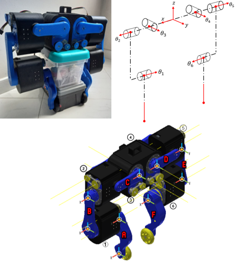
IV Kinematic model
The development of the kinematic model of the bipedal robot BLUE was raised from the transformation matrices of Denavit-Hartenberg, for which the lower right-limb support was established as the point of origin, this, in order to resemble the process of locomotion in the walk to that of the human being, in which the kinematic chain begins in the ankle, passes through the hip and ends in the opposite ankle.
| (11) |
The kinematic model was constructed from the parameters required for the construction of the general transformation matrix described by Denavit Hartenberg evidenced in the Equation 11 , in which all the frames, in addition to being in agreement with the different degrees of freedom, aligned the rotation axes (z) in such a way that along the structure, the displacement and rotation was uniform.
Figure 7shows variations from 0 to 15 degrees in each of the different degrees of freedom present in the BLUE kinematic chain, which are the beginning of the chain in the right support (th0), the knee of the right limb, located more specifically in the actuator (1) and one of the abductions present in the hip with the help of the actuator (4).

V Dynamical model (Euler-Lagrange)
BLUE robot have six degrees of freedom. The vector contains the angles to be varied, where and are the angles of the knees flexion, and are the angles of the legs extension, and are the angles of the hip abduction. The location of each of the angles can be seen in the Figure 6.
Generalized coordinates are:
| (12) |
The positions of the centers of mass of the six bodies are:
| (13) |
Where varies according to the body ( and ), is the position in x axis, is the position in y axis and is the position in z axis. (Equation 13).
The velocity vectors () are calculated for each body.
V-A Calculation of the Lagrangian
The Lagrangian is defined in the Equation 14, where is the kinetic energy and is the potential energy.
| (14) |
The angular velocity and inertial matrices are calculated, can be seen in the Equation 15 and Equation 16.
| (15) |
| (16) |
- •
Kinetic energy
Total kinetic energy is calculated in Equation 17. Where the sub-indice indicate the kinetic energy on each body ( and ).
(17) The kinetic energy of the bodies can be written in a generalized form (Equation 18):
(18) - •
Potential energy
The total potential energy is calculated in Equation 19
(19) Potential energy of the bodies can be written in a generalized form (Equation 20):
(20) Where is the mass of each body, is the gravity and is the height of each body.
With the total kinetic and potential energies are proceed to calculate the Lagrangian (Equation 14).
V-B Lagrange differential equation
The Lagrange differential equation is described in Equation 21.
| (21) |
Partial derivative of the Lagrangian with respect to the partial derivative of velocity.
Partial derivative of the Lagrangian with respect to the partial derivative of position.
The generalized forces are:
Where is the torque generated from the gear motor output, the viscous damping coefficient and the velocity vector.
Motor torque is defined as:
| (22) |
The input voltage is described in Equation 23.
| (23) |
The electromotive force () is proportional to the angular velocity of the motor (), is the armature current, is the armature resistance, is armature inductance, is the voltage across the armature inductance, is the torque constant and is the against-electromotive constant.
Finally, the Euler-Lagrange equation is described in the Equation 24.
| (24) |
Matrix off mass and inertia
Coriolis and centripetal effects
Stifness and gravitationals effects
Input
V-C Simulation of the dynamical model
In the Figure 8, it is observed the simulation of dynamic model to zero input, it is visualized with particularity that Theta 1 () reaches approximately 90°, because it is simulated as if it fell to the ground and bounced to stand still.
It is also observed that the position of Theta 3 () falls to -35° which is equivalent to 0.6 radians approximately, this means that since the hip is slightly tilted with respect to the ground, its final position at rest is tilted.

V-D Proposed control
It is proposed a non-linear control designed for the three-dimensional movement of the BLUE robot, where there are six control inputs which drive the system. The proposed control scheme has matrix , and the vector .
The higher-order derivative is solved as of Euler-Lagrange model and obtained Equation 25.
| (25) |
The proposed control law for signal of each gear motor is described as:
Where and the error it’s defined to:
Velocity error ().
The desired acceleration.
The desired velocity.
the desired position.
Measured velocity.
Measured position.
A stabilization time of was defined with a dominant pole at and a polo five times faster . The gains of the control system are and . Tracking of the desired trajectory is checked, making use of the proposed control system. Follow up of the desired trajectories can be evidenced in Figure 9.

VI Experimental test
The repetitive movement of each of the joints was developed to verify compliance in the mobility of each BLUE joint, as a support, video capture was made, which is observed in Figure 10 fragmented for its correct visualization. Within these practices standard resources such as an Arduino Nano and L298N module.

Figure 11shows the encoder reading of the hip actuator where the angle varies from to degrees.

VII Conclusions
A 3D bipedal robot was designed and fabricated using a mechatronics designing approach. To reduce the impact effects on the support-foot exchange event, a flexible serial actuator was developed. Additionally, a reduction of the mass was performed with a generative design approach, which uses topology optimization to define the shape of the robot’s shins. These mechanisms and parts were successfully fabricated and implemented using 3D-printed parts. The bipedal robot was evaluated numerically and a prototype was fabricated to validate the design.
The preliminary results from the design of a nonlinear control with feedback linearization show acceptable performance in tracking trajectories.
References
- [1] Q. Huang, S. Kajita, N. Koyachi, K. Kaneko, K. Yokoi, H. Arai, K. Komoriya, and K. Tanie, “A high stability, smooth walking pattern for a biped robot,” in Proceedings 1999 IEEE International Conference on Robotics and Automation (Cat. No. 99CH36288C), vol. 1, pp. 65–71, IEEE, 1999.
- [2] M. Gienger, K. Loffler, and F. Pfeiffer, “Towards the design of a biped jogging robot,” in Proceedings 2001 ICRA. IEEE International Conference on Robotics and Automation (Cat. No. 01CH37164), vol. 4, pp. 4140–4145, IEEE, 2001.
- [3] J. Weng, “Creación del modelo del robot humanoide teo para el simulador webots,” B.S. thesis, 2012.
- [4] H.-W. Park, K. Sreenath, J. W. Hurst, and J. Grizzle, “Identification and dynamic model of a bipedal robot with a cable-differential-based compliant drivetrain,” University of Michigan Control Group, Tech. Rep. CGR, pp. 10–06, 2010.
- [5] C. Hubicki, J. Grimes, M. Jones, D. Renjewski, A. Spröwitz, A. Abate, and J. Hurst, “Atrias: Design and validation of a tether-free 3d-capable spring-mass bipedal robot,” The International Journal of Robotics Research, vol. 35, no. 12, pp. 1497–1521, 2016.
- [6] J. Arcos-Legarda, J. Cortes-Romero, and A. Tovar, “Robust compound control of dynamic bipedal robots,” Mechatronics, vol. 59, pp. 154–167, 2019.
- [7] J. Arcos-Legarda, J. Cortes-Romero, A. Beltran-Pulido, and A. Tovar, “Hybrid disturbance rejection control of dynamic bipedal robots,” Multibody System Dynamics, vol. 46, no. 3, pp. 281–306, 2019.
- [8] J. W. Hurst, The role and implementation of compliance in legged locomotion. Carnegie Mellon University, 2008.
- [9] A. Ramezani, J. W. Hurst, K. Akbari Hamed, and J. W. Grizzle, “Performance analysis and feedback control of atrias, a three-dimensional bipedal robot,” Journal of Dynamic Systems, Measurement, and Control, vol. 136, no. 2, p. 021012, 2014.
- [10] A. Hattori, Design of a high torque density modular actuator for dynamic robots. PhD thesis, Massachusetts Institute of Technology, 2020.