Operator backflow and the classical simulation of quantum transport
Abstract
Tensor product states have proved extremely powerful for simulating the area-law entangled states of many-body systems, such as the ground states of gapped Hamiltonians in one dimension. The applicability of such methods to the dynamics of many-body systems is less clear: the memory required grows exponentially in time in most cases, quickly becoming unmanageable. New methods reduce the memory required by selectively discarding/dissipating parts of the many-body wavefunction which are expected to have little effect on the hydrodynamic observables typically of interest: for example, some methods discard fine-grained correlations associated with -point functions, with exceeding some cutoff . In this work, we present a theory for the sizes of ‘backflow corrections’, i.e., systematic errors due to discarding this fine-grained information. In particular, we focus on their effect on transport coefficients. Our results suggest that backflow corrections are exponentially suppressed in the size of the cutoff . Moreover, the backflow errors themselves have a hydrodynamical expansion, which we elucidate. We test our predictions against numerical simulations run on random unitary circuits and ergodic spin-chains. These results lead to the conjecture that transport coefficients in ergodic diffusive systems can be captured to a given precision with an amount of memory scaling as , significantly better than the naive estimate of memory required by more brute-force methods.
I Introduction
Transport properties, such as heat, charge and spin conductivities, are among the most experimentally accessible and practically important features of materials, and also serve to distinguish the plethora of phases of condensed matter. Yet, our ability to predict these properties from first principles in interacting quantum matter is limited. Improving existing methods has the potential to facilitate sharper predictions for existing experiments, aid in the exploration and discovery of new phenomena, and allow the design of future experimental systems with bespoke transport properties.
Even in the linear response regime, the calculation of transport properties requires computing unequal time correlation functions, and thus depends on our ability to simulate the dynamics of quantum many-body systems. Unsurprisingly, existing methods like exact evolution Heitmann et al. 2020, and time-evolved block decimation (TEBD) Verstraete et al. 2008 are strongly limited for such ab initio studies. Exact evolution is limited to small systems sizes, while estimates from TEBD are limited to just a few interaction times before the memory requirements become impractical/truncation errors become significant Schollwöck 2011; Paeckel et al. 2019.
Recently, a number of methods have been proposed for sidestepping these issues White et al. 2018; Parker et al. 2019; Prosen and Žnidarič 2009; Kvorning et al. 2021; Rakovszky et al. 2020; White 2021; Wurtz et al. 2018. All of these methods (with the exception of Ref. Prosen and Žnidarič 2009) rely on the intuition that much of the information content of a many-body density matrix – particularly correlation functions involving products of many-operators Rakovszky et al. 2020, or operators with large spatial support White et al. 2018; White 2021; Kvorning et al. 2021; Wurtz et al. 2018 – can be thrown away without greatly affecting the calculation of transport coefficients. This intuition has been articulated in various forms for decades in (for example) the formulation of the BBGKY hierarchy, and the approximations employed in the mode-coupling/memory-matrix formalism and fluctuating hydrodynamics approaches to many-body systems Reichman and Charbonneau 2005; Landau and Lifshitz 1987 .
It is apparent from the references above that many investigators believe that the general approach of discarding complicated correlations should give good approximate results. These expectations have been largely supported by numerous (but by no means systematic) numerical calculations which show impressive convergence requiring surprisingly few computational resources White et al. 2018; Parker et al. 2019; Prosen and Žnidarič 2009; Kvorning et al. 2021; Rakovszky et al. 2020. Here ‘surprisingly few’ means the calculations produce accurate estimates (seemingly to within a few percent) of transport coefficients using only modestly powered classical computers; one might have expected that such many-body quantum problems generically require the use of a quantum computer for accurate results.
A detailed understanding of the sizes of systematic errors for these methods is lacking, however. In other words, if one does discard higher order correlations, what is the size of the resulting systematic errors in the estimates of transport coefficients? Answering this question requires us to understand the size of backflow processes, wherein information from higher order correlations ‘flows back’ to the subspace of local observables.
The present paper aims to remedy this gap in the literature. Although our results are relevant to various recently proposed methods White 2021; White et al. 2018; Kvorning et al. 2021, our primary interest is in the dissipation assisted operator evolution (‘DAOE’) method Rakovszky et al. 2020. For DAOE, the correlation functions are approximated by modifying unitary Heisenberg dynamics so that operators with support on, say, more than sites are discarded or strongly dissipated. While we have highlighted the issue of estimating transport coefficients, our results are also relevant to the numerical simulation of hydrodynamical correlation functions (HCFs) which can shed light on more general non-equilibrium processes, such as quantum quenches.
We principally study ergodic systems in 1D with a single U conserved density undergoing diffusion, although we also expect our results to apply to systems for which the only conserved quantity is energy. In such a system, HCFs are expected to have an expansion in of general form
| (1) |
For example in spatial dimensions, if is chosen to be the local charge density, then and for a diffusion constant . We develop a physical picture for how HCFS are modified when DAOE dissipation is applied (Eq. (14)). This physical picture leads to a prediction: The difference, or backflow, induced in Eq. (1) by using DAOE also has a hydrodynamical expansion
| (2) |
Inspired by the study of random circuits, we argue that the leading order contributions to backflow are exponentially suppressed in . In other words . Moreover, our hydrodynamical theory of backflow corrections also predicts the leading order exponent for the time decay of corrections in Eq. (2). It turns out that the predicted value depends on the hydrodynamical operator , and whether or not the system has spatiotemporal randomness (like random circuits), but in all cases the backflow corrections decay at least as quickly as the original correlation function, i.e., .
These results lead to the conclusion that the error induced in the diffusion constant due to the DAOE protocol is exponentially small in
| (3) |
We support our theoretical predictions with a numerical study of deterministic systems (Fig. 2), although naturally this study is plagued by the usual memory limitations that impede our simulation of many-body systems, and so these results are not decisive. We supplement it with a study of backflow in the U-symmetric random unitary circuit (RUC) (Fig. 5). Specifically, we compute the average effect of DAOE dissipation on the charge diffusion coefficient and various correlation functions. The advantage of using random circuits is that circuit-averaged quantities can be mapped to statistical mechanics models, which tend to be easier to simulate to longer times and for larger systems sizes than would be available by simulating real-time dynamics directly Rakovszky et al. 2018. We also provide further consistency checks of our hydrodynamical picture for backflow corrections using a semi-analytical treatment of circuit averaged dynamics in a U(1) RUC.
As we detail in Sec. VI, our backflow picture implies that accurate estimates of diffusion constants can be obtained by restricting dynamics to a smaller effective Hilbert space – the space of short operators. This in turn implies that DAOE dramatically reduces the memory required to estimate transport coefficients. To be more precise, we reason that -accurate approximations to transport coefficients can be obtained using DAOE in combination with matrix product operators with relatively small bond dimension . In contrast, a naive estimate suggests that the standard more brute-force approaches (TEBD, exact evolution) require substantially higher bond dimension . Therefore, in the limit , DAOE is far more memory efficient than these existing approaches.
This work is organized as follows. Sec. II reviews conventions, and describes the DAOE protocol. Sec. III summarizes the expected behavior of hydrodynamical correlation functions without any truncation. Sec. IV develops a theory for the form of backflow corrections due to DAOE, explaining their exponential suppression in and time dependence, and presents numerical results (Fig. 2) supporting this picture. Sec. V then investigates backflow in a U random circuit, presenting numerical results (Fig. 5) which further support the picture in Sec. IV, as well as a semi-analytical calculation demonstrating that a subclass of backflow corrections are exponentially suppressed in . Sec. VI uses the theoretical picture in Sec. IV to argue that DAOE substantially reduces memory overheads compared to more brute-force approaches (asymptotically). We conclude and present future directions in Sec. VII.
II Setting and conventions
We focus on 1D ergodic lattice systems at high temperature, with local unitary dynamics and possessing a single conserved density which diffuses. For much of the discussion, and for concreteness, we will take our system to be a spin-1/2 chain, and for the conserved quantity to be the total -component of the spin, namely (which can equivalently be interpreted as the charge of hard-core bosons). We denote the local magnetization by , so that . We expect our results to generalize to the study of energy diffusion in systems with a local Hamiltonian. The ergodicity requirement eliminates certain finely-tuned models (like Bethe-Ansatz integrable models), and localized systems. Our requirement that the conserved quantity diffuses is not very restrictive, given the ubiquity of systems exhibiting diffusion at high temperatures Bloembergen 1949; Gennes 1958; Kadanoff and Martin 1963.
It is useful to define an inner product between operators ; throughout this paper we work at infinite temperature, so that . This turns the space of operators in to a Hilbert space; as we shall see, it is natural to phrase various transport-related quantities in this language. For example, dynamical correlations are equivalent to an inner product between an operator at time and another at time .
The unitary matrix evolves states from time . For energy conserving systems time is a continuous variable and where is the Hamiltonian. For Floquet/random circuit systems, time is a discrete variable. Moreover, for Floquet systems for Floquet unitary . Unitary time evolution acts on density matrices via a superoperator , so that the expectation value of a Hermitian observable can be written
where is the density matrix at some earlier time . In this work, we focus on the structure of time evolved operators, which evolve according to the Heisenberg picture
Our primary object of study is the diffusion constant. It can be written as where the time-dependent diffusion constant is defined as
| (4) |
An exact calculation of is limited by the exponential growth of Hilbert space dimension with system size, with numerical studies limited to spins at most Heitmann et al. 2020. One may instead attempt to evaluate Eq. 4 using TEBD, representing the time-evolved operator as a matrix product operator (MPO). However, as increases, the bond dimension needed for a high fidelity MPO representation of also grows. In particular, for the ergodic systems we consider, it is expected that the corresponding operator entanglement grows linearly with Jonay et al. 2018, making the memory requirements grow exponentially, as .Therefore one needs an approximation scheme in order to be able to accurately evaluate at long times. Recently, several such approximation schemes were proposed that rely on an idea of ‘operator truncation’ Rakovszky et al. 2020; Kvorning et al. 2021; White 2021. The shared intuition between these methods is that information regarding the component of on operators that are highly non-local can be safely discarded, as these are are believed to have little quantitative effect on hydrodynamics.
In the following, we focus on one particular such approximation scheme, termed DAOE, that was introduced in Ref. Rakovszky et al. 2020 by the present authors. DAOE is implemented as follows. We estimate the diffusion constant or hydrodynamical correlation functions using a modified time evolution. In addition to the unitary Heisenberg evolution, we apply a superoperator with time period that suppresses operators longer than some cutoff length , i.e., in Eq. (4), we replace with (assuming is integer) and where . The original DAOE dissipator is most easily defined in terms of its action on Pauli strings , which form a basis in the space of all operators acting on the spin chain. The dissipator then takes the form
| (5) |
where – the ‘length’ of operator – is the number of non-identity matrices in the string 11 1 This quantity is known as the Pauli weight in quantum computing literature.. Using this nomenclature, note that the operator has length , even though it is spread over a large spatial region (of diameter ). It will also be useful to define the superoperator
The DAOE dissipator may then be written . The DAOE dissipator has a compact MPO representation, which is important for the implementation of the DAOE procedure on tensor product representations of operators Rakovszky et al. 2020.
With dissipation present, we obtain in general a different estimate for the diffusion constant which we denote as
| (6) |
, and . Note that this expression is identically equal to if or , since the dissipation is switched off in both of these limits. We also note that while the method depends on the parameter , one can show Rakovszky et al. 2020 that in the limit of small , it is only the ratio that matters; we therefore fix to some value and vary . We will assume that exceeds the length of operators contained in , which ensures that the DAOE dynamics at least conserve ; in most cases we consider, this simply requires . Our goal will be to estimate the size of
| (7) |
as is increased further.
III Summary of diffusive hydrodynamics
Before turning to our main topic of estimating backflow corrections, it is worth first clarifying how correlation functions behave in the absence of truncation, in the long-time regime where hydrodynamics holds sway Forster 2018. While these results are well known, we are not aware of any reference that presents all the facts that we require for our analysis, so we will need to synthesize results from multiple works Forster 2018; Mukerjee et al. 2006; Khemani et al. 2018; Lux et al. 2014; Chen-Lin et al. 2019; Glorioso et al. 2021 into a unified picture.
At long times, the correlation functions between local operators are dominated by the slowest operators with which they can develop an overlap under time evolution. In other words, the correlation function can be approximated as
| (8) |
at leading order in , and up to multiplicative constants.
The physical idea underpinning Eq. (8) is similar to that of the operator product expansion in quantum field theory Delacrétaz 2020. Using the language developed in the previous section, we can explain it as follows. We choose some appropriate basis of operators (not necessarily Pauli strings), which we denote , and write
| (9) |
where we assume time-translation invariance and . Here, is some short time scale that depends on the size of . The sum in Eq. (III) will be dominated by the basis operators with slowly decaying correlations. In particular, we expect to leading order in . At large , the sum in Eq. (III) will be dominated by the smallest . The exception is if there is a cancellation between terms with the same ; however, this can be avoided by making an appropriate choice for the basis , which will be dictated by the choice of .
Eq. (8) can be illustrated with the following picture:
| (10) |
Here contracts down to in some time, which then propagates until a time close to , at which point the operator grows to form . It will turn out that, modulo a few special cases and caveats we will shortly mention, the slowest variable is the local density if . Otherwise, it is the spatial gradient of the density . Readers willing to take this on trust may skip the remainder of this section, which serves to justify this result.
In the systems studied here, operators are subject to diffusive hydrodynamics, i.e.,
| (11) |
where is a function whose width scales as , and takes approximate scaling form in the diffusive limit in spatial dimensions. It further obeys due to the fact that is a conserved quantity 22 2 To simplify notation, we will occasionally lapse into using continuum notation rather than their more cumbersome lattice analogues..
What are the slowest hydrodynamical variables? Natural candidates involve products of ’s and spatial derivatives, which we denote as (the notation suppresses the details of how the spatial derivatives are distributed among the ’s, and the regularization of the product ). According to naive dimension counting, this variable will have autocorrelation functions decaying as . That is because each pair of ’s is associated with a single factor of the propagator , while diffusive scaling implies . Thus, according to this naive dimension counting, the slowest variables are those with as few powers of as possible. In spatial dimensions (our main focus), the four most relevant variables are which by dimension counting decay as respectively.
will play a special role in what follows. While is not the slowest of all hydrodynamical variables, it turns out that many operators are prevented from developing an overlap with by symmetry constraints. These constraints arise from the fact that the overlap of an operator with the total spin (or indeed any function of the spin) is independent of time because the operator is exactly conserved under time evolution.
We will illustrate this point with a few examples of operators , applying Eq. (8) and symmetry constraints to predict the long-time behavior of their correlation function. If , then the answer is already clear. by definition. As noted, this decays at late times as .
If on the other hand , then the answer is more interesting. The component of on single operators can be written as a superposition for some function . However, as is orthogonal to the total spin, we have the constraint that , which implies that this can be rewritten as with supported in the light-cone. The conclusion is that cannot develop a component of that survives coarse-graining. Similarly, is orthogonal to , which (after coarse-graining) precludes developing an overlap with the next slowest operators .
These considerations show that the slowest hydrodynamical operator with which can develop an overlap is . Thus we expect . If , the same style of argument shows that .
Returning to the case of operators of form , recall that their autocorrelations decay as according to naive dimension counting. However, this does not always correctly predict the decay of correlations for operators involving many ’s. That is because such operators can (in accordance with Eq. (8)) develop an overlap with slower hydrodynamical variables involving a product of fewer ’s, and as a result decay slower than would be expected from dimension counting. However, the question of which hydrodynamical variables can develop an overlap is once again constrained by symmetry: The situation for is summarized in Fig. 1.
The same reasoning leads to a more general principle, useful for later discussions in this work. If are operator strings orthogonal to , and both are local and charge neutral (i.e., commute with ), then should hold at large , up to multiplicative constants. In other words, is the slowest hydrodynamical variable with which can develop overlap 33 3 In , the same statement holds but one can drop the requirement of orthogonality with . In one may additionally drop the requirement of orthogonality with ..
Finally, we note that if an operator has with (i.e., the operator creates/destroys charge), then can never have an overlap with any hydrodynamical variable. That is because all the hydrodynamical variables mentioned above commute with , and
| (12) |
for any operators . In words, the adjoint action of commutes with time evolution. In the absence of additional slow modes in the system, such a variable is expected to have exponentially decaying correlations.
This section has focused on the case where the sole conserved quantity is a U charge. While we think our main conclusions generalize to systems with energy conservation and to finite temperature, some of the details (particularly those involving operator overlaps) may change44 4 We thank Luca Delacretaz for a related discussion..
IV Theoretical picture for backflow contributions
In this section, we present a theoretical justification for our central claim: systematic errors (e.g., Eq. (7)) due to DAOE are exponentially small in . Our strategy is as follows. We first consider a stripped-down version of the question: What is the effect on a hydrodynamic correlation function of discarding all operators above some length half-way through the evolution (at time )? We will call this quantity and we shall argue that it is exponentially suppressed in . Then, in Sec. IV.4, we argue that this result extends to the case of periodically applied dissipation.
IV.1 A single dissipation event
Our first aim is to bound the quantities
| (13a) | ||||
| (13b) | ||||
where are local operators based around positions respectively. Here is a projector onto all operators of length . Similarly is a projector onto all operators greater than length ; these quantities measure the contributions to from ‘backflow’ type processes where the operator grows to a significant size () and then shrinks back to .
The hydrodynamical picture of Eqs. (8) and (10) suggests how to bound Eq. (13) at long times. We contend that the leading contributions take the form
| (14) |
In words, decays into a hydrodynamical operator , which propagates until a time near . It then grows so as to satisfy the length constraint imposed by the projector with , before contracting back to a hydrodynamical operator, which propagates to as before. It will be sufficient for us to consider the case where are both orthogonal to , so that the dotted line corresponds to the propagation of a single , with .
The growth/contraction process is represented by the grey box (which we refer to as ) and occurs over a time-scale which is in turn set by ; note that this time scale will need to be at least as long as to give the hydrodynamic operator sufficient time (set by a Lieb-Robinson bound) to grow to length . The initial and final spatial locations will need to be summed over, but they are forced by locality and the relative smallness of to be close to one another.
The resulting process will decay with a power law in , coming from the diffusive propagators (dotted lines) making up Eq. (14). The precise exponent of this power law can be determined using the hydrodynamical rules discussed in Sec. III; we will do this in the next section.
However, the key point is that the process will be additionally suppressed by the amplitude associated with the grey box. It is this suppression that allows us to isolate the dependence of Eq. (13). Our claim, which we support with both analytical arguments and numerical results below, is that such amplitudes are exponentially suppressed in . After summing the contributions over all , it follows that is exponentially small in as required.
There are various assumptions made in the picture presented above. The key idea is that the grow-shrink process represents an excursion out of the space of small operators, and the longer the excursion, the harder it is for the operator to find its way back to a small hydrodynamical operator. This idea leads to the statement above that is set by rather than (which is equivalent to the fast decay of with ), and also responsible the exponential suppression of in .
IV.2 Estimating
We now present a quantitative justification of this idea. To see why is exponentially suppressed in , introduce a resolution of the identity at time :
| (15) |
where we sum over all operators of length , and the ’s are transition amplitudes. For example, is the amplitude for to evolve to operator over time ; we have dropped the explicit dependence of to simplify the notation.
IV.2.1 Dynamics without conserved quantities
We first note that there are good theoretical reasons to expect amplitudes of form Eq. (15) to be small in a system without any conservation laws (including conservation of energy). Operator spreading in such models have been studied in Refs. Nahum et al. 2018; von Keyserlingk et al. 2018 (see also Ref. Nahum et al. ming). In this case, a natural expectation is that the summand in Eq. (15) has a randomly fluctuating sign as a function of . That allows us to make the approximation
| (16) | ||||
| (17) |
Using the sum rule for a normalized operator , we can further bound this by
| (18) |
One can further justify this equation by an analytical calculation in Haar random unitary circuits of the kind employed in Refs. von Keyserlingk et al. 2018; Nahum et al. 2018, where taking the average of Eq. (16) leads to exactly.
Considering the RHS of Eq. (18), we note that there are exponentially many operators of length in the forward light cone of . Since we assumed no conservation laws, one expects that these all occur with roughly equal amplitudes, which readily gives the required exponential suppression of . Once again, this can be verified explicitly in random circuits (see e.g., Eq. (C2) in von Keyserlingk et al. 2018). In that case, one finds that the result is exponentially decaying both in and in .
IV.2.2 Systems with U symmetry
The preceding argument is well controlled (e.g. it can be made exact in random circuits), but flawed because it ignores the role of continuous symmetries in the grow/shrink processes. To address that problem, we want to consider a system which has a single conservation law associated to a U symmetry (we still exclude energy conservation). Paradigmatic models of this kind can be constructed as random unitary circuits where the structure of the local gates is restricted by the symmetry. Khemani et al. 2018; Rakovszky et al. 2018. We shall study such a circuit model in detail in Sec. V; here we give a more heuristic argument.
When continuous global symmetries are present, the path from Eq. (16) to Eq. (17) becomes less controlled, (even in the aforementioned U circuits, we do not have exact expressions for the circuit-averaged operator spreading coefficients). Nevertheless, we now argue (non-rigorously) that the final result (exponential suppression in ) continues to hold. Intuitively, the symmetry qualitatively changes the behavior of processes that involve relatively short operators, leading to the diffusive (rather than exponential) decay of correlations. However, despite the underlying symmetry, it still seems reasonable (and in-line with existing works Rakovszky et al. 2018; Khemani et al. 2018) to assume that the amplitudes governing the ballistic growth of operators are somewhat random, so that an argument analogous to that presented above still holds.
An operator appearing in Eq. (15) can be expressed as a tensor product of on-site operators of form . Separate out the part of and call it . Likewise separate out the components (which can only have support on sites not already occupied by ), calling it . Then . For example, the string has and . Within the random circuit calculation, can be non-vanishing (on average) only if , while are allowed to differ. This gives a generalization of the random-phase approximation above, and one which we expect to hold approximately for more general U-symmetric models as well. Another constraint is that, as is hydrodynamical it is also charge neutral. That is equivalent to requiring the number of ’s is equal to the number of ’s in .
For simplicity of presentation, we restrict ourselves to estimating with . Once more we isolate those backflow corrections due to operators of some size (we will eventually sum over ). We will assume that, as in the previous case without conservation laws, is some function of alone, rather than the long time scale in Eq. (13). We define the size of the effective light cone where is a Lieb-Robinson velocity. The processes contributing to require that , because the grow/shrink process should produces operators of length at least part-way through the evolution.
Starting from Eq. (16), and using gives
| (19) |
where is the length of . The dash on the sum over indicates that must be even (so that is charge neutral). We now make a further approximation: the coefficients have roughly the same size for all that are supported within a ball of diameter of . In other words, for given length , the operator spread coefficients of operators supported in are to a good approximation independent of the detailed content of the operator e.g., independent of and the particular locations of operators. This approximation refines an existing picture Ho and Abanin 2017 so as to include some of the effects of charge conservation.
We can now perform the sums, picking out combinatorial factor . After that, we perform the sum, giving factor . The result is
| (20) |
where . To estimate the RHS of this equation, we note the sum rule . Using the same approximations leading to Eq. (20), this bound may be expressed as
| (21) |
The sum on the RHS of Eq. (21) has been estimated using a saddle point approximation and the assumption of large . The upshot is that is bounded above by the inverse of the number of operators of length within the region of width . We can now bound Eq. (20) using Eq. (21) to give
| (22) |
The supremum is achieved for . Thus, if we assume operators of length have somewhat uniform operator spreading coefficients for large , it is natural that backflow processes are exponentially suppressed in . The final step of this argument involves summing Eq. (22) over contributions for all , with the end result result is that the backflow due to a single dissipation event is exponentially suppressed in
The above argument makes the assumption that is set by . It also assumes that the size of operator spread coefficients to operators of fixed length, within a forward causal cone, are to good approximation uniform, which is certainly not true in general. Therefore, it behooves us to perform additional consistency checks on the results in this section. We will perform multiple checks. First, we investigate numerically our backflow hypothesis in some ergodic (non-random) spin chains (see Fig. 2). Later, in Sec. V we will give a more detailed analysis of the U-symmetric random circuit model. In that case, we can evaluate backflow contributions at long times numerically (see Fig. 5); all of these checks agree with our prediction of exponentially suppressed backflow effects. Moreover, the numerical checks in Fig. 2 suggest that our arguments apply to systems for which the conserved quantity is energy rather than the U charge assumed in this section. Finally, we will lend further support to our hypothesis by evaluating analytically certain sub-classes of contributions to in the random circuit model and showing that they are consistent with that quantities’ exponential suppression in and the conjecture that is set only by .
IV.2.3 Numerical checks in deterministic spin chains
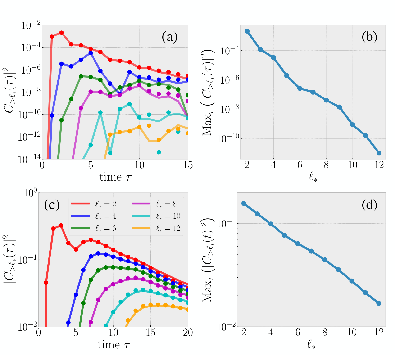
In order to support our argument, here we investigate backflow in two deterministic models (tilted-field Ising and XX ladder) studied using DAOE in our previous work Rakovszky et al. 2020, as well as in numerous other works using alternative methods Leviatan et al. 2017; Kvorning et al. 2021; Steinigeweg et al. 2014; Kloss et al. 2018. We investigate the quantity , as applied to the autocorrelation function of a conserved density (energy in the Ising case, and -magnetization for the ladder). Both cases are consistent (Fig. 2) with our conjecture that decays exponentially in , although the data are certainly less clean and decisive than those calculated using random circuits.
We first consider the tilted-field Ising model
| (23) |
fixing and . The model is expected to be strongly chaotic Karthik et al. 2007; Kim and Huse 2013. is the energy associated to site . This is the only local conserved density in the model, and its correlations capture energy (or heat) transport Kim and Huse 2013. We represent as an MPO and evolve it using the TEBD method Vidal 2003. We calculate the quantity which is the version of the quantity defined in Eq. (13), where we used that the dynamics generated by Eq. (23) is time-reversal invariant.
The results are shown in Fig. 2a,b. First, we perform the calculation for various values of . is suppressed at early times, , by the Lieb-Robinson bound. At that time, it grows and reaches a peak value; at late times it decays again. While the data is rather noisy, we clearly observe that the curves corresponding to large ( is the largest we consider) are strongly suppressed compared to ones with smaller . To quantify this, we consider the maximum of over the range of we access and plot it as a function of in Fig. 2b. The results are well fit by the exponential decay we predict theoretically; there is a difference of about 7 orders of magnitude in going from to .
We also consider a spin- model on a two-leg ladder Steinigeweg et al. 2014; Karrasch et al. 2015; Kloss et al. 2018. We denote by the rungs of the ladder, and use for the two legs. Pauli operators on a given site are specified as , etc. The Hamiltonian then reads
| (24) |
Besides energy, this model also conserves the spin component, . We calculate as above, with replaced by the average magnetization on a rung, . We plot the results in Fig. 2c,d. We find that the trends with are cleaner than in the Ising model, although their magnitude is much smaller. In particular, we find that results are only suppressed by about a factor of compared to ; nonetheless, they are very well fit by an exponential decay.
IV.3 Hydrodynamical expansion for backflow corrections
We have argued that backflow processes are exponentially suppressed in . We now determine the dependence of quantities like Eq. (14) on time. The answer will depend both on the structure of and on whether or not the system is noisy (e.g., a random circuit system). We will verify our predictions using simulations of backflow in the U(1) RUC (Fig. 5); our deterministic data (Fig. 2) do not go to sufficiently long times to test our predictions for time dependence.
As discussed in Sec. III, without any truncation the correlator decays with some power determined by the slowest hydrodynamical variables with which (respectively) have overlap. When we examine the effects of a single truncation event Eq. (13), we force the operators to be of size part way through their evolution. Thus, at least for the purposes of understanding time dependence, we expect the leading power in to be determined by a correlator of form
| (25) |
where is some operator of length , localized near both . is the ‘grey box’ amplitude associated with the grow/shrink process. As long as , is the slowest hydro operator with which can develop overlap. Therefore we expect backflow corrections Eq. (14), fixing , to have the same temporal decay as . Simple power counting, or substituting in an explicit form for the hydrodynamical correlators Eq. (11), shows that this decays as . [Note from that scales as . Furthermore, in diffusive systems ].
However, to fully account for the backflow processes contributing to Eq. (13), we will need to integrate over intermediate positions . Here, the results will strongly depend on whether the system has randomness, in other words whether the grow/shrink amplitude represented by the grey box in Eq. (14) depends on individually, rather than just their difference.
In systems without such randomness, the integration is straightforward, and gives rise to an additional power of , so that Eq. (13) scales as , which decays faster than the original correlation function by a power of . The exponential suppression in is encoded in .
In systems with randomness, relevant to the random circuits we study numerically, the grow/shrink amplitude will have a random sign dependent on position . On average, the contribution to Eq. (25) will be zero, but its typical modulus will scale as the standard deviation
| (26) |
The scaling in time of Eq. (26) follows immediately from dimension counting, and takes form , which decays a factor of faster than in the case without noise. Once again, the exponential suppression in is provided by the factor.
Combining our results so far, we can evaluate the backflow correction to a diffusion constant Eq. (4) due to a single dissipation event:
| (27) |
We thus have to integrate our results over . Estimating the result is straightforward: When there is no noise, . When there is noise, the result show scale as . We test this latter prediction in Fig. 5(a,b) below.
IV.4 Periodic dissipation
So far we examined the effect of a single dissipation event on a correlation function, with the conclusion that the error introduced by dissipation is exponentially suppressed in . What effect do multiple applications of a dissipator have on correlators (e.g., as would be required to calculate Eq. (6))? In other words, we want to estimate the error
| (28) |
where and . We will use our hydrodynamical picture of backflow processes to argue that is exponentially suppressed in for all . From this it follows (integrating over ) that . For simplicity, we will be satisfied with showing that is exponentially suppressed; the computation for finite goes through in the same way provided one assumes that DAOE dissipation does not change the fact that the system undergoes diffusion (our previous work Rakovszky et al. 2020 supports this assertion).
The derivative with respect to is
| (29) |
The summand here is similar to Eq. (13), and for the same reasons suppressed exponentially in . The novelty in the present calculation is that we must sum over times at which we insert the projector 55 5 Note are the same up to a polynomial factor in ; hence whether we apply or part way through the evolution will not affect whether the contribution decays exponentially in .
Using the hydrodynamical assumptions above, we represent the derivative as
| (30) |
A result from a previous section is that for each fixed , Eq. (30) is exponentially decaying in and also suppressed by a further factor when there is no spatial randomness, and by a factor when there is.
When there is no randomness in space or time, we therefore expect the backflow correction due to be of order ; so the correction due to backflow is exponentially decaying in but has the same power of as the original correlation function.
When there is randomness in space and time, we need to integrate over time, taking into account the fact that the sign of the integrand will fluctuate randomly in time ( now depends randomly on as well as ). The result of that integral is an enhancement, giving a result .
The same reasoning can be applied to quantities like the diffusion constant.
| (31) |
When there is no noise, simple dimension counting indicates that this term goes as ; i.e., it represents a correction to the diffusion constant which decays exponentially with because does. Integrating over leads to the statement that .
When there is noise, we must account for the fluctuating signs of . In this limit, Eq. (31) may be approximated as
| (32) |
Dimension counting, and integrating over , predicts that which is indeed exponentially decaying in . We test this hypothesis numerically in Fig. 5(c,d), for the U-symmetric random circuit model.
In summary, we have shown that the backflow corrections to hydrodynamical quantities are accompanied by an exponential suppression in , and a power law which depends on whether or not the system has randomness, and which hydrodynamical correlation is being considered. In all cases, however, the backflow correction decays in time at least as quickly as the original hydrodynamical correlation function.
V U random circuit analysis
| Rule | Input example | Rule Output |
|---|---|---|
| 0 | ||
| 1 | ||
| 2 | ||
| 3 | ||
| 4 | ||
| 5 | ||
| 6 | ||
| 7 |
In this section, we supplement our argument above with a more thorough analysis of a U symmetric random circuit model and use it to estimate Eq. 13 both numerically and analytically. Along the way, we will see how the dynamics of U RUCs agrees with the hydrodynamical picture just explained.
The random circuit model is defined as follows. The random unitary circuit has a brick-work structure (see also Fig. 3)
| (33) |
Each acts exclusively on sites . Moreover, for each , is a matrix drawn independently from some ensemble. We will consider the case where each is Haar random, subject to the constraint that it commutes with the global U symmetry , endowing it with the block structure shown in Fig. 3. This ensemble has been useful in capturing the OTOC/operator spreading Khemani et al. 2018; Rakovszky et al. 2018 and entanglement growth properties of systems with continuous conservation laws, capturing novel behaviors that appear to be present even in the absence of randomness Khemani et al. 2018; Rakovszky et al. 2018; Rakovszky et al. 2019. In this specific random circuit model, plays the role of our conserved density, thus we use the two interchangeably in our discussions of numerical results.
V.1 Circuit-averaged dynamics
We now turn to the task of estimating backflow. As was shown in Refs. Khemani et al. 2018; Rakovszky et al. 2018, on average there is no backflow in the random circuit: averages to zero. This is due to a cancellation between different circuit realizations. Instead, we want to understand the size of backflow contributions in typical realizations. To this end, we examine , which can be recast as
| (34) |
where we use compact notation . The denotes a tensor product between the two replica copies needed to calculate the squared quantity, while the denotes a tensor product between different sites. Here , and recall that represents the adjoint action of the unitary on an operator. Recall that our circuits consist of two-site gates chosen independently for each position and time-step. Since all gates in the circuit are chosen independently, we can perform averages over them separately. After averaging, we are left with an effective Markovian evolution, which is generated by a circuit averaged super-operator . This object is a large () matrix; it is a linear map on tensor product pairs of operators. However, it is a projector and has a small (13-dimensional) support spanned by the states in the third column of Fig. 4 and their symmetry related partners (and ), and thus admits a relatively simple description.
In particular, while the on-site Hilbert space in this replica-doubled problem is dimensional, states in the support of can be entirely described by the following operator pairs
Note that operators of form as well as (and their two additional replica swapped versions) do not appear here: they are annihilated by the evolution operator. The intuitive explanation for this result is that operator pairs that locally change charge are associated with rapidly fluctuating phases whose contributions tend to vanish under averaging. This sort of phenomenon is well-known in ergodic non-random systems where, for example, particle propagators develop a finite lifetime (e.g., exponential decay of with time in a high temperature Bose-Hubbard model). This idea was used above to arrive at Eq. (19) and consequently to argue for exponential suppression of backflow.
The transition amplitudes induced by a single two-site averaged gate have been calculated previously Khemani et al. 2018; Rakovszky et al. 2018 and are summarized in Fig. 4. The evolution is simply a sum of projectors onto the states in the rule output column and their symmetry related states, which can be obtained by globally swapping or or . These three symmetries reflect the inversion symmetry of the random ensemble, and (for the final two rules) the fact is invariant under swapping replicas.
Let us list some other important observations concerning the rules 0-6:
- •
Isolated ’s undergo diffusion (rule 1); but they cannot diffuse past one another (rule 2); in other words they undergo single file diffusion. Similarly for ’s
- •
Except when they meet, tend to random walk (rules 4,5 and their symmetry related versions).
- •
As random walk, they are equally likely as not to emit pairs.
- •
Both of can absorb pairs or inter-convert . play a crucial role in processes that change the total number of operators: they constantly attempt to produce pairs, and they are the only operators that can absorb other operators.
It is useful to note that rules 0-6 define a probability conserving classical stochastic process, on a state space where each site takes one of six values. Only rule 7 breaks this pattern, because some of its transition amplitudes are negative. Rule 7 dictates what happens when meet, and determines (in combination with rule 3) what happens when meet:
| (35a) | ||||
| (35b) | ||||
Note that the right hand sides of Eq. (35a) and Eq. (35b) involve a sum of contributions from two of the rules (3 and 7) in Fig. 4, because the left hand sides have overlap with the corresponding two states in the output column.
Due to the non-probability conserving nature of rule 7, Eq. 35 have some negative amplitudes and the weights on the RHS of the equations need not sum up to as they do for rules 0-6. Nevertheless, these rules show that pairs can fuse to form a pair. Similarly, when meet, they have some chance of forming an pair.
We can now summarize and synthesize these observations together into a simpler story. For each time step that an are present in an operator, that operator will tend to grow in support because constantly tend to emit pairs. This process is difficult to reverse because the produced can only be absorbed by , but are most likely to diffuse away from their parent . Thus tend to lead to further operator growth. This manifests itself in a finite lifetime/exponentially decaying in time return probability for a pair; we verify this story in more detail later (Sec. V.4).
V.2 Numerical results
Using the update rules summarized in Fig. 4 for every gate in the circuit we arrive at a process that is formally analogous to a classical stochastic many-body evolution, albeit with some negative transition ‘probabilities’. One can then use this representation to evaluate quantities like the average squared correlator numerically. For this involves taking an initial configuration with on site and everywhere else, evolving under the rules of Fig. 4, and then considering the ‘probability’ (overlap) associated to a configuration with a single on site . Following previous works Rakovszky et al. 2018; Rakovszky et al. 2019, one can do this in a tensor network language, representing the instantaneous distribution as a MPS and updating it using TEBD; it was found previously that the effective bond dimension in this problem does not grow very rapidly, allowing one to get reliable results for times and system sizes well beyond the reach of naive exact evolution.
One can easily extend this calculation to the backflow contribution, . In order to do so, one only has to insert at time into the evolution. This allows us to evaluate the size of backflow corrections in the random circuit more reliably than we were able in the deterministic spin chains studied in Sec. IV.2.3. This is further helped by the fact that the randomness of the circuit makes diffusive behavior set in immediately, while for a fixed Hamiltonian there is some short local thermalization time before which hydrodynamics does not apply.
In Fig. 5a,b we plot the U circuit average of , i.e., the error suffered by the diffusion constant due to a single dissipation event, as defined in Eq. (27). In the top panel, we plot this quantity against time for different . The data are consistent with a power law with decay exponent close to our prediction of ; the fit is not decisive, although it can be much improved by allowing for a sum of power laws ( and ) which can be easily accounted for by our hydrodynamical formalism. An alternative hypothesis, which the numerical simulations do not rule out but which is inconsistent with theory, is that there is power law decay with an exponent between and . In the bottom panel (b), we plot the same quantity as a function of for various values of , rescaling all results by . The results appear consistent with exponential decay in .
In Fig. 5c,d we plot the average value of , the error in the diffusion constant when the dissipation is applied after every two layers of the circuit. We again find that the error decays algebraically in time. Here the fit is of a better quality and we extract an exponent of decay from the data that is , in good agreement with our prediction of . Panel (d) also shows evidence of exponential decay in , although we were not able to test larger in this case for want of computational resources.
V.3 Consistency with hydrodynamical picture
The update rules above also allow us to estimate some of the backflow contributions analytically. But first, to develop some intuition, we will show how to recover from them the hydrodynamical picture presented in Sec. III.
Let us examine the circuit averaged behavior of
| (36) |
a correlator in the absence of any dissipation events. Take to be local strings of that are charge neutral (i.e., each has the same number of and ). Consider the limit of very large (in comparison to the lengths of ). In this limit, represents the amplitude for a local operator to evolve to another local operator over a long period of time.
We have already mentioned tend to lead to further operator growth. On the other hand, undergo single-file diffusion, which is a slow/hydrodynamical process. Thus, we expect the leading order behavior of Eq. (36) in to involve the propagation of these slow operators.
| (37) |
The grey triangles in Eq. (37) represent processes whereby the initial/final operators contract into . Unless the is already a single , said processes necessarily involve the propagation and annihilation of pairs and so are short-lived (in comparison to ). For example, if we choose , a will need to be generated (using rule 7) in order to on net remove three of the pairs (using rule 4)
| (38) |
On the other hand if we choose then the operator begins with a pair; these will annihilate quickly (compared to ) through rule 7:
| (39) |
These examples illustrate a general point; unless have overlap with , one needs to use rule 7 in order to reduce the operator down to an pair 66 6 We ignore the special situation where have overlap with , in which case it may not be favorable to reduce the operator to an pair.. However, note that rule 7 produces in the combination , which includes two spatial derivatives. This is consistent with the finding in Sec. III, namely that unless overlap with , then the slowest variable with which they can develop overlap is .
V.4 pairs are short-lived
In this section we argue that the survival probability of a pair of ’s decays rapidly with time. Concretely, we conjecture that the amplitude
| (40) |
decays faster than any power law, and we provide an argument for a stretched exponential decay . Our numerical simulation of the circuit average of Eq. (40) (see Fig. 6) is consistent with this. The object is the same as except we set to zero all matrix elements which would allow a pair to convert into ; this is a modification to rule 7. Thus Eq. (40) represents the amplitude that the pair (initially on sites ) persist for time , and propagate back to their initial positions.
It is worth reminding the reader how Eq. (40) behaves if we do not insist the pair persist. In this case, we are examining
| (41) |
which decays as . That is because Eq. (41) is just the square of , which decays as according to the hydrodynamical recipe in Sec. III. In the related construction Sec. V.3, the power law comes from processes were the pair combine to , which then propagate diffusively. A circuit averaged simulation of Eq. (41) (Fig. 6) is consistent with the predicted power law.
We now give a theoretical picture explaining why Eq. (40) decays as a stretched exponential. As evolves the pair, they will diffuse, and in the process source pairs (according to rule 3). The number of that can be created is diffusion-limited because the diffuse, and at most one and at most one an occupy a given site. As a result, by time we expect to have number of , distributed in a region of size centered on the origin. The equal probability of removing versus adding a pair of from a or (rule 3) suggests that the density of in this diffusive cone approaches a steady state limit 77 7 Our argument only requires that the density approaches a limit strictly between .. We will assume that, to a good approximation, each site within the diffusive cone has independent probability of being occupied by and .
We are studying the overlap which represents the rare event where at the last time step no are present. The probability that no are present are, from the reasoning in the previous paragraph, expected to scale as , which is the stretched exponential result we wished to prove. Note we have thus far ignored the requirement that the pair return to the origin. This will further suppress the amplitude by an unimportant power law in .
Perhaps the least controlled assumption in the argument above is that we have ignored processes where can fuse and form pairs (additional to the original pair). We cannot rigorously argue that such processes are irrelevant for obtaining the stretched exponential, however it is at least self-consistent to ignore such processes: they give rise to pairs which we are arguing (and have demonstrated numerically) are short-lived. As an aside, we note that the argument for stretched-exponential decay is almost identical to the one presented in our previous work Rakovszky et al. 2019 showing that higher Rényi entropies grow diffusively, a result that can be proved independently under mild assumptions Huang 2020.
V.5 A subset of backflow corrections
Our discussion in Sec. IV.1 identifies the exponential suppression of growth/shrinkage processes as being the source of exponential suppression in backflow due to DAOE. This suppression is easy to prove in the RUC without symmetry. We are unable to rigorously prove exponential suppression in the U(1) RUC. We can, however, examine the contributions of certain sub-classes of process contributing to backflow. In other words, our aim here is to use the U(1) RUC model to estimate a subset of the contributions to as defined in Eq. (14).
Specifically, we examine the contributions of growth/shrinkage processes where the control parameter is the number of applications of Rule 7. This choice is made primarily because it affords control over the diagrammatic expansion, but also because the processes contributing are irreducibly rely on the diffusive modes that distinguish the U(1) RUC from the RUC without symmetry.
Rule 7 must be used twice in a growth process (it is required both at the beginning and end of the grow/shrink process). An example of such an amplitude (which would contribute for ) is
| (42) |
Amplitudes of this type require a single pair to persist for time . However, we have argued in Sec. V.4 that such processes are suppressed as . Moreover, in the same section, we argued that the operator support tends to increase diffusively, so that . The net conclusion is that such processes are suppressed as (and after we sum over ). As a result, the subset of processes of form Eq. (42) are consistent with our main assumption in previous sections, namely that grow-shrink processes contributing to are exponentially suppressed in .
We can also estimate the contributions of diagrams involving a few more applications of rule 7. For example the following amplitudes has four such applications
| (43) |
In processes involving four applications of rule , at least one of the two pairs formed must survive for at least time in order to increase the support of the operator to part-way through the evolution. But the pairs released will need to be absorbed, and this is once again unlikely. The same reasoning as above shows that this amplitude is suppressed as once summed over all .
We have argued that the first few orders in a series expansion are consistent with the exponential decay of backflow. It may be that this mode of reasoning can be extended order-by-order to diagrams that involve further applications of rule 7, however we were unable to prove rigorously that the fully summed series is on net exponentially suppressed in . Our limited numerical evidence (Fig. 5) suggests that the fully summed series of contributions will continue to show exponential decay in , but a complete proof is lacking and could be an interesting topic for future investigation.
VI How hard is it to simulate quantum transport classically?
We now discuss the implications of our various conjectures for numerical studies of dynamics in many-body systems. We will be interested in the following question: What resources are required to compute transport properties, such as a diffusion constant, to some fixed precision ?
A standard approach for calculating the diffusion constant – used in exact evolution and tensor-network based methods – is to approximate the true diffusion constant with a finite time approximation. The deviation between the diffusion constant and its finite time approximation is bounded as where is an constant 88 8 This follows from the Drude formula and the fact that current auto-correlations decay as Mukerjee et al. 2006; we focus on in this section.. Thus we will need to simulate the system for a minimum time in order to obtain an estimate for to within tolerance .
For exact evolution, we must consider a finite-sized systems, say with sites. In order to avoid incurring significant finite-size effects, the corresponding Thouless time ought to exceed : This translates to the requirement , although one can only prove rigorously that finite-size effects are exponentially suppressed in (and thus much smaller than ) if we use the stricter condition for some Lieb-Robinson scale . In either case, if we wish to obtain an accurate approximations to the diffusion constant, we will require , which leads to a memory requirement .
In tensor network methods, we need not work with finite systems. However, the entanglement of the time-evolved state/operator is expected to increase linearly in time on theoretical grounds Jonay et al. 2018. This suggests – and experience confirms – that bond dimension needed to control the errors in local observables grows exponentially with time. Using , this would lead to a bond dimension requirement scaling as . It is possible this bound is too pessimistic: in the small limit, it might be possible to leverage the diffusive nature of the transport and truncate the support of our time evolved state/operator to a region of size , which would reduce the bond dimension requirement to . In either case, we expect that the bond dimension requirement scales as
| (44) |
which is in-line with the memory requirements for exact evolution.
Modifying the dynamics with DAOE dissipation significantly reduces the memory overhead. This is especially clear in the strong dissipation limit, , where we explicitly restrict the accessible Hilbert space to operators with length ; however, it was found in Ref. Rakovszky et al. 2020 that even when and are both finite, DAOE limits the growth of operator entanglement to a value that remains bounded at all times. The cost is that we introduce a systematic error in the diffusion constant; however, as we argued throughout this paper, this error is bounded by . Insisting that the systematic error is less than requires . We still have the requirement that . For times of this order, the accessible Hilbert space at is . For small , this implies that the bond dimension required for a tolerance calculation of the diffusion constant scales as
| (45) |
which is significantly less than either the memory requirement for tensor network simulations in the absence of dissipation in Eq. (44) or that of exact evolution discussed above.
While it is generally believed that some dynamical properties of quantum many-body systems are not efficiently simulable on classical computers Preskill 2012; Aaronson and Chen 2017; Arute et al. 2019, our result Eq. (45) suggests that transport properties are (at least in ergodic systems). It would be interesting to find what other problems fall into this latter category, and devise new classical algorithms to tackle them.
VII Conclusion
We have argued that the ‘backflow’ contributions to hydrodynamic correlations involving operators that act on more than different sites are exponentially suppressed in (Sec. IV.1). Moreover, the corrections to correlation functions and transport coefficients due to backflow are themselves arranged in a series in powers of ; we have made various predictions for the exponents of these contributions, dependent on whether the systems have randomness, and the hydrodynamical correlation function in question (Sec. IV.3). We have provided numerical evidence for this picture, both in deterministic quantum spin chains (Fig. 2), and in U symmetric random circuit models (Fig. 5). In the latter case, we provided further semi-analytical consistency checks of both our hydrodynamical picture for backflow corrections as well as the assertion that backflow corrections are exponentially suppressed in (Sec. V). Our conjectured bounds have important consequences for the asymptotic computational resources required for ab initio calculation of transport properties; our results suggest that the DAOE method introduced in Ref. Rakovszky et al. 2020 requires significantly smaller numerical resources than existing established methods like ED or TEBD (see e.g. Eqs. (44) and (45) in Sec. VI).
This work leaves many questions open. It would be worthwhile to generalize the theoretical predictions in this work to finite temperatures/chemical potentials. It is likely that a dramatic modification to these results occurs in higher dimensions at sufficiently low temperatures such that the systems undergo an ordering transition. Moreover it is worth performing a backflow analysis for a variety of truncation methods (including truncating dependent of the spatial support rather than the length of operators); we plan to explore this in forthcoming work.
In this paper, we focused on one-dimensional systems. Nonetheless, we expect the hydrodynamical framework developed here to apply in higher dimensions; in particular, we expect our arguments in Sec. V.4 for exponential suppression with to generalize quite straightforwardly. We note that it may be practicable to use DAOE in this more general setting, given recent advances in higher dimensional tensor network algorithms. It would be interesting to investigate the growth/shrinkage processes in higher dimensions and with greater detail and control. Forthcoming work by Nahum et al. goes in this direction, with a focus on grow-shrink processes in the random circuit without symmetries Nahum et al. ming.
It would also be interesting to connect our results to existing efforts in the study of complexity theory. Various results are known on the computational resources required to, e.g., calculate the ground state energy density of local Hamiltonians Aharonov and Irani 2021; Watson and Cubitt 2021. What can be said for the calculation of hydrodynamical quantities? Our results arguably indicate that, at least for ergodic systems (which are ubiquitous), surprisingly few resources are required. Finally, there are certainly many conjectures and technical points in the present work which would benefit from further study. For example, can one prove rigorously that backflow is exponentially suppressed in the U(1) circuit averaged model?
VIII Acknowledgements
We thank Luca Delacretaz, Christopher White, Daniel Parker and Gabriele Pinna for useful discussions. CvK is supported by a UKRI Future Leaders Fellowship MR/T040947/1. The computations described in this paper were performed in part using the University of Birmingham’s BlueBEAR HPC service. F.P. acknowledges support from the European Research Council (ERC) under the European Union’s Horizon 2020 research and innovation programme (grant agreement No. 771537) and the Deutsche Forschungsgemeinschaft (DFG, German Research Foundation) under Germany’s Excellence Strategy EXC-2111-390814868 and TRR 80. T.R. is supported by the Stanford Q-Farm Bloch Postdoctoral Fellowship in Quantum Science and Engineering. TR acknowledges the hospitality of the Aspen Center for Physics, supported by National Science Foundation grant PHY-1607611 and the Kavli Institute for Physics, supported by the National Science Foundation under Grant No. NSF PHY-1748958.
References
- Heitmann et al. (2020) T. Heitmann, J. Richter, D. Schubert, and R. Steinigeweg, Zeitschrift für Naturforschung A 75, 421 (2020).
- Verstraete et al. (2008) F. Verstraete, V. Murg, and J. Cirac, Advances in Physics 57, 143 (2008), https://doi.org/10.1080/14789940801912366 .
- Schollwöck (2011) U. Schollwöck, Annals of Physics 326, 96 (2011), january 2011 Special Issue.
- Paeckel et al. (2019) S. Paeckel, T. Köhler, A. Swoboda, S. R. Manmana, U. Schollwöck, and C. Hubig, Annals of Physics 411, 167998 (2019).
- White et al. (2018) C. D. White, M. Zaletel, R. S. K. Mong, and G. Refael, Physical Review B 97 (2018), 10.1103/physrevb.97.035127.
- Parker et al. (2019) D. E. Parker, X. Cao, A. Avdoshkin, T. Scaffidi, and E. Altman, Phys. Rev. X 9, 041017 (2019).
- Prosen and Žnidarič (2009) T. Prosen and M. Žnidarič, Journal of Statistical Mechanics: Theory and Experiment 2009, P02035 (2009).
- Kvorning et al. (2021) T. K. Kvorning, L. Herviou, and J. H. Bardarson, “Time-evolution of local information: thermalization dynamics of local observables,” (2021), arXiv:2105.11206 [quant-ph] .
- Rakovszky et al. (2020) T. Rakovszky, C. W. von Keyserlingk, and F. Pollmann, “Dissipation-assisted operator evolution method for capturing hydrodynamic transport,” (2020), arXiv:2004.05177 [cond-mat.str-el] .
- White (2021) C. D. White, “Effective dissipation rate in a liouvillean graph picture of high-temperature quantum hydrodynamics,” (2021), arXiv:2108.00019 [cond-mat.str-el] .
- Wurtz et al. (2018) J. Wurtz, A. Polkovnikov, and D. Sels, Annals of Physics 395, 341 (2018).
- Reichman and Charbonneau (2005) D. R. Reichman and P. Charbonneau, Journal of Statistical Mechanics: Theory and Experiment 2005, P05013 (2005).
- Landau and Lifshitz (1987) L. D. Landau and E. M. Lifshitz, Fluid Mechanics (1987).
- Rakovszky et al. (2018) T. Rakovszky, F. Pollmann, and C. W. von Keyserlingk, Phys. Rev. X 8, 031058 (2018).
- Bloembergen (1949) N. Bloembergen, Physica 15, 386 (1949).
- Gennes (1958) P. D. Gennes, Journal of Physics and Chemistry of Solids 4, 223 (1958).
- Kadanoff and Martin (1963) L. P. Kadanoff and P. C. Martin, Annals of Physics 24, 419 (1963).
- Jonay et al. (2018) C. Jonay, D. A. Huse, and A. Nahum, “Coarse-grained dynamics of operator and state entanglement,” (2018), arXiv:1803.00089 [cond-mat.stat-mech] .
- Forster (2018) D. Forster, Hydrodynamic fluctuations, broken symmetry, and correlation functions (CRC Press, 2018).
- Mukerjee et al. (2006) S. Mukerjee, V. Oganesyan, and D. Huse, Physical Review B 73 (2006), 10.1103/physrevb.73.035113.
- Khemani et al. (2018) V. Khemani, A. Vishwanath, and D. A. Huse, Physical Review X 8 (2018), 10.1103/physrevx.8.031057.
- Lux et al. (2014) J. Lux, J. Müller, A. Mitra, and A. Rosch, Physical Review A 89 (2014), 10.1103/physreva.89.053608.
- Chen-Lin et al. (2019) X. Chen-Lin, L. V. Delacrétaz, and S. A. Hartnoll, Physical Review Letters 122 (2019), 10.1103/physrevlett.122.091602.
- Glorioso et al. (2021) P. Glorioso, L. V. Delacrétaz, X. Chen, R. M. Nandkishore, and A. Lucas, SciPost Phys. 10, 15 (2021).
- Delacrétaz (2020) L. Delacrétaz, SciPost Physics 9 (2020), 10.21468/scipostphys.9.3.034.
- Nahum et al. (2018) A. Nahum, S. Vijay, and J. Haah, Phys. Rev. X 8, 021014 (2018).
- von Keyserlingk et al. (2018) C. W. von Keyserlingk, T. Rakovszky, F. Pollmann, and S. L. Sondhi, Phys. Rev. X 8, 021013 (2018).
- Nahum et al. (ming) A. Nahum, S. Roy, S. Vijay, and T. Zhou, “Chaos and the time-ordered two-point function,” (forthcoming).
- Ho and Abanin (2017) W. W. Ho and D. A. Abanin, Phys. Rev. B 95, 094302 (2017).
- Leviatan et al. (2017) E. Leviatan, F. Pollmann, J. H. Bardarson, D. A. Huse, and E. Altman, “Quantum thermalization dynamics with matrix-product states,” (2017), arXiv:1702.08894 .
- Steinigeweg et al. (2014) R. Steinigeweg, F. Heidrich-Meisner, J. Gemmer, K. Michielsen, and H. De Raedt, Phys. Rev. B 90, 094417 (2014).
- Kloss et al. (2018) B. Kloss, Y. B. Lev, and D. Reichman, Phys. Rev. B 97, 024307 (2018).
- Karthik et al. (2007) J. Karthik, A. Sharma, and A. Lakshminarayan, Phys. Rev. A 75, 022304 (2007).
- Kim and Huse (2013) H. Kim and D. A. Huse, Phys. Rev. Lett. 111, 127205 (2013).
- Vidal (2003) G. Vidal, Phys. Rev. Lett. 91, 147902 (2003).
- Karrasch et al. (2015) C. Karrasch, D. M. Kennes, and F. Heidrich-Meisner, Phys. Rev. B 91, 115130 (2015).
- Rakovszky et al. (2019) T. Rakovszky, F. Pollmann, and C. von Keyserlingk, Physical Review Letters 122 (2019), 10.1103/physrevlett.122.250602.
- Huang (2020) Y. Huang, 1, 035205 (2020).
- Preskill (2012) J. Preskill, arXiv preprint arXiv:1203.5813 (2012).
- Aaronson and Chen (2017) S. Aaronson and L. Chen, in 32nd Computational Complexity Conference (CCC 2017), Leibniz International Proceedings in Informatics (LIPIcs), Vol. 79, edited by R. O’Donnell (Schloss Dagstuhl–Leibniz-Zentrum fuer Informatik, Dagstuhl, Germany, 2017) pp. 22:1–22:67.
- Arute et al. (2019) F. Arute, K. Arya, R. Babbush, D. Bacon, J. C. Bardin, R. Barends, R. Biswas, S. Boixo, F. G. S. L. Brandao, D. A. Buell, B. Burkett, Y. Chen, Z. Chen, B. Chiaro, R. Collins, W. Courtney, A. Dunsworth, E. Farhi, B. Foxen, A. Fowler, C. Gidney, M. Giustina, R. Graff, K. Guerin, S. Habegger, M. P. Harrigan, M. J. Hartmann, A. Ho, M. Hoffmann, T. Huang, T. S. Humble, S. V. Isakov, E. Jeffrey, Z. Jiang, D. Kafri, K. Kechedzhi, J. Kelly, P. V. Klimov, S. Knysh, A. Korotkov, F. Kostritsa, D. Landhuis, M. Lindmark, E. Lucero, D. Lyakh, S. Mandrà, J. R. McClean, M. McEwen, A. Megrant, X. Mi, K. Michielsen, M. Mohseni, J. Mutus, O. Naaman, M. Neeley, C. Neill, M. Y. Niu, E. Ostby, A. Petukhov, J. C. Platt, C. Quintana, E. G. Rieffel, P. Roushan, N. C. Rubin, D. Sank, K. J. Satzinger, V. Smelyanskiy, K. J. Sung, M. D. Trevithick, A. Vainsencher, B. Villalonga, T. White, Z. J. Yao, P. Yeh, A. Zalcman, H. Neven, and J. M. Martinis, 574, 505 (2019).
- Aharonov and Irani (2021) D. Aharonov and S. Irani, “Hamiltonian complexity in the thermodynamic limit,” (2021), arXiv:2107.06201 [quant-ph] .
- Watson and Cubitt (2021) J. D. Watson and T. S. Cubitt, “Computational complexity of the ground state energy density problem,” (2021), arXiv:2107.05060 [quant-ph] .