Analysis and Design of Distributed MIMO Networks with a Wireless Fronthaul

A user $k$ located in cell $q$, i.e., $k\in{\mathcal{U}}_{q}$ and served by the RRH cluster $\mathcal{D}_{q}$, receives the signal

where $s_{qk}\in\mathbb{C}$ is the unit-energy symbol sent to user $k$ by the serving RRHs. The vector ${\bf h}_{qnk}^{*}\in\mathbb{C}^{M}$ denotes the channel between RRH $n$ in cell $q$ and user $k$. We model ${\bf h}_{qnk}$ as

where ${\bf g}_{qnk}\sim\mathcal{CN}({\bf 0},{\bf I}_{M})$ represents the small-scale fading and $\ell_{k}(x_{qn},y_{qn})=\left(1+d_{qnk}/d_{0}\right)^{-\alpha}$ represents the path loss, with $d_{qnk}=\sqrt{(x_{qn}-\widetilde{x}_{k})^{2}+(y_{qn}-\widetilde{y}_{k})^{2}}$ the distance between RRH $n\in\mathcal{D}_{q}$ and user $k$, $d_{0}$ the reference distance, $\alpha$ the path loss exponent, and $\beta_{qnk}$ denotes the shadowing. The terms $(x_{qn},y_{qn})$ denote the x and y coordinates of RRH $n$, while the vector ${\bf w}_{qnk}\in\mathbb{C}^{M}$ denotes the precoding vector used by RRH $n$ for user $k$. Finally, $z_{qk}\sim\mathcal{CN}(0,\sigma_{z}^{2})$ denotes the additive white Gaussian noise (AWGN) with average power $\sigma^{2}_{z}$.

We define the concatenation of the channel matrix for all the users in cell $q$ as ${\bf H}_{q}^{*}\triangleq[{\bf h}_{q1}^{*}\dots{\bf h}_{qK}^{*}]\in\mathbb{C}^{NM\times K}$, with ${\bf h}_{qk}^{*}=[{\bf h}_{q1k}^{H}\dots{\bf h}_{qNk}^{H}]^{T}$ being the length-$NM$ concatenation of the channels between the $N$ RRHs in cell $q$ and user $k$. We can write ${\bf h}_{qk}\triangleq{\bf D}_{qk}^{1/2}{\bf g}_{qk}$, where ${\bf D}_{qk}\in\mathbb{C}^{NM\times NM}$ is a diagonal matrix representing the large-scale fading between all the RRHs in cell $q$ and user $k$. Hence, $[{\bf D}_{qk}]_{mm}=\beta_{qnk}\ell_{k}(x_{qn},y_{qn})$ where $n=\lceil{m/M}\rceil$, for $m=\{1,\dots,NM\}$. Correspondingly, ${\bf g}_{qk}\in\mathbb{C}^{NM}$ represents the vector of the small-scale fading coefficients between the antennas of the RRHs in cell $q$ and user $k$.

The precoding matrix designed for cell $q$ is defined as ${\bf W}_{q}=[{\bf v}_{q1}\dots{\bf v}_{qK}]\in\mathbb{C}^{NM\times K}$ with ${\bf v}_{qk}=[{\bf w}_{q1k}^{T}\dots{\bf w}_{qNk}^{T}]^{T}\in\mathbb{C}^{NM}$, where ${\bf w}_{qnk}\in\mathbb{C}^{M}$ is defined above. We use ZF linear precoding on the access channel. With the CSI known, the precoding matrix is formed as

where $\bm{\mu}_{q}\in\mathbb{C}^{K\times K}$ allows us to satisfy the power constraint. As done in [24, 25], we use a vector normalization, allowing for a fair comparison across network configurations. Hence, $\bm{\mu}_{q}$ is a diagonal matrix such that $\mathbb{E}\left\{\text{tr}\left\{{\bf W}_{q}{\bf W}_{q}^{H}\right\}\right\}=p$; its $k^{th}$ diagonal entry is defined as

with ${\bf\widetilde{v}}_{qk}=\left[{\bf\widetilde{W}}_{q}\right]_{.k}=\left[{\bf H}_{q}\left({\bf H}_{q}^{H}{\bf H}_{q}\right)^{-1}\right]_{.k}$, i.e., the $k^{th}$ column of ${\bf\widetilde{W}}_{q}$. Note that we assume the matrix ${\bf H}_{q}$ is full-row rank, an assumption that is valid with probability one [24].

The ZF beamformer used for the access channel is constructed for each cell $q$, thereby canceling intra-cluster interference. Based on the normalization in (4), the average signal power received at user $k\in\mathcal{U}_{q}$ in cell $q$ is $\mu_{qk}^{2}$. Under our assumption of perfect CSI, one lower bound on the achievable spectral efficiency, measured in nats/s/Hz, is [26]

We note that, through the channel powers, this spectral efficiency is a function of the distances between the RRHs found in the network and user $k$, (later on the RRH locations which will be our optimization variables). The expectation in (5) is over the small-scale fading realizations and user locations.

Since user locations are unknown at the system design stage, we treat user locations as random, and hence we assume that their statistics are represented through a spatial traffic distribution (assumed known). This distribution inside a specific network area can be constructed using passive monitoring of mobile users in the network regions, which can be located through location areas, sectors, cells, etc. Then the hotspots in the network can be identified from the collected data. This distribution can also be built from very extensive and complex surveys performed for the network, such as identifying the locations of the crowded areas (e.g., stadiums, campuses, etc), and analyzing spatio-temporal activity of the users. All in all, our study is only concerned with the step of representing the spatial traffic distribution using a series of convex combinations, and hence we do not elaborate in detail on the methods of collecting the spatial statistics from an actual network; readers can refer to papers that specifically target this topic such as the survey in [27].

Let the concatenated form of the RRH locations in the network be written as $\left[{\bf x},{\bf y}\right]$, where the x-coordinates are ${\bf x}=[{\bf x}_{1}^{T},\dots,{\bf x}_{q}^{T},\dots,\dots,{\bf x}_{Q}^{T}]^{T}$ (and similarly for ${\bf y}$). We use $[{\bf x}_{q},{\bf y}_{q}]$ to refer to the locations of the RRHs in cell $q$, where ${\bf x}_{q}=[x_{q1}\ \dots\ x_{qN}]^{T}$. We also use $[{\bf x}_{-q},{\bf y}_{-q}]$ to refer to the locations of all the RRHs in the network other than in cell $q$. Using this notation, this lower-bound of the achieved spectral efficiency on the access channel for a typical user $k$ served by the disjoint cluster $\mathcal{D}_{q}$ is [3]

with

Here, ${I}^{(a)}_{q^{\prime}k}({\bf x}_{q^{\prime}},{\bf y}_{q^{\prime}})$ denotes an average inter-cluster interference (ICI) term. We begin with

where $\rho=\frac{p}{\sigma_{z}^{2}}$ and $\xi(q^{\prime},j)=\text{tr}\{{\bf D}_{q^{\prime}j}\}=M\sum_{m\in\mathcal{D}_{q^{\prime}}}\beta_{q^{\prime}mj}\ell_{j}(x_{q^{\prime}m},y_{q^{\prime}m})$. The RRHs in an interfering cell $q^{\prime}$ contribute $\check{I}^{(a)}_{q^{\prime}k}({\bf x}_{q^{\prime}},{\bf y}_{q^{\prime}})$ to the total inter-cell interference. This interference term depends on the random locations of the users in the interfering cells because the beamformers in each cell is designed based on the channels of these users. Let $(\widetilde{x}_{k},\widetilde{y}_{k})$ denote the location of typical user $k$. To obtain the average ICI on the access channel, we use a spatial traffic probability density function (PDF) $f_{q}(\widetilde{x}_{k},\widetilde{y}_{k})$ to model the user locations, resulting in

where $\mathcal{B}_{q^{\prime}}$ denotes the boundary of cell $q^{\prime}$. The PDF $f_{q}(\widetilde{x}_{k},\widetilde{y}_{k})$ can be constructed from a traffic survey, and it allows us to represent the density of users at any coordinate $(\widetilde{x}_{k},\widetilde{y}_{k})$. Later in the paper, we will elaborate on how to define $f_{q}(\widetilde{x}_{k},\widetilde{y}_{k})$. The derivation of (6) from (5) can be found in [3, Appendix A].

In summary, (6)-(9) provide a lower bound on the access rate to a typical user as a function of the locations of the RRHs. These rates are possible only if the fronthaul can sustain them. In the next two sections, we use our network model to analyze two possible fronthaul schemes: multicast and ZF beamforming. The choice of ZF and multicast beamforming is based on their tractability, in addition to their low computational complexity and low coordination requirements between the CUs compared to counterpart numerical beamforming techniques. Wireless multicasting is appropriate since all RRHs in a cell require the data of all $K$ users they serve, i.e., all $N$ RRHs are to receive the same data. However, as we will see, multicasting is effective only for a small number of $N$. For large $N$, we must use ZF beamforming in the fronthaul.

Due to fading, the multicast fronthaul rate is random and hence, we can only place a probabilistic outage constraint on the fronthaul. This, in turn, requires a statistical analysis of the signals received on the fronthaul. Specifically, we impose the constraint

where $\omega$, $\omega_{\rm b}$ are the bandwidth allocated for the data plane for the access channel and fronthaul respectively, and $\epsilon$ denotes the allowed fronthaul outage probability. The constraint sets the probability of outage to be less than a chosen value of $\epsilon$. Here, $R_{qn}^{\rm{(b)}}\left({\bf x}_{q},{\bf y}_{q}\right)=\log\big(1+\frac{S_{qn}^{(b)}}{I_{qn}^{(b)}+\sigma_{z}^{2}}\big)$ denotes the achievable rate on the fronthaul. We must work with the minimum rate in the fronthaul because all $N$ RRHs must receive the data for the users. The right hand side of the inequality denotes the average rate to the $K$ users, with

where $\mathcal{B}_{q}$ is the boundary of cell $q$. The probabilistic outage constraint for the fronthaul in (16) cannot be directly used to optimize the location of the RRHs, hence some simplification is needed. A natural approach is to use some reference distribution to characterize this constraint. To do this, we fit the signals received at the RRHs on the fronthaul with a reference distribution, then we use this framework to characterize the constraint in (16).

We apply the KS test on the signals received at the RRHs on the fronthaul. This test compares a sample statistic with a reference distribution to reject (null hypothesis) or accept the hypothesis that the sample was drawn from the reference distribution. Hence, it estimates the goodness of the fit. In Fig. 3, we plot the average number of times the null hypothesis was retained.

For the test setup, we use $Q=9$ square cells with wraparound (to eliminate network boundary effects), where the CU for each cell is found at the cell center, i.e., the CUs are located on a grid. Each cell contains $N=10$ RRHs randomly deployed in the cell with an exclusion region of $20$ meters around the CU. Other details on the network setup can be found in Table I. We generate Monte Carlo simulations for $100$ network realizations, each has $1000$ channels realizations. We then apply the KS test to each set of channel realizations using many reference distributions, shown in Fig. 3. Finally, we obtain the average number of times that the null hypothesis was retained in, i.e., we obtain the average number of times in which the hypothesis that the samples came from the reference distribution was rejected.

Our results show that the gamma distribution has the lowest null hypothesis tests obtained from our Monte Carlo simulation. Thus, the gamma distribution is the best fit for the different beamforming techniques. Based on this, we will derive accurate closed-form expressions for the mean and variance of the power of the desired signal and interference. Then, we will relate these moments to the parameters of the gamma distribution to analytically perform the fitting.

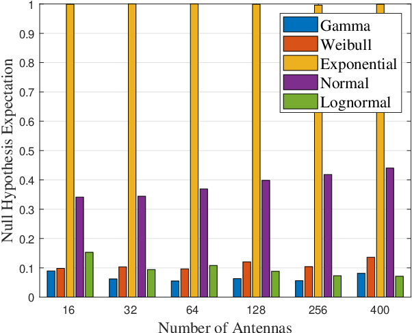
Based on this discussion, we model the desired signal and interference powers at each RRH as a gamma RV $Y$, which is characterized by shape ($K_{Y}$) and scale ($\theta_{Y}$) parameters where

We therefore need the mean and variance of the signal and interference powers to characterize the gamma distribution. However, unlike other studies using a similar model that use numerical methods [6, 35], we provide accurate, if approximate, closed-form expressions for these moments.

The received SINR at the fronthaul of RRH $n$ is

To obtain a closed-form expression for the constraint in (15), we use the fact that $R_{qn}^{\rm{(b)}}<\dot{\mathsf{x}}$ if $S^{\rm{(b)}}_{qn}<(e^{\dot{\mathsf{x}}}-1)(I^{\rm{(b)}}_{qn}+\sigma_{z}^{2})$ i.e., $\mathbb{P}\left\{R_{qn}^{\rm{(b)}}<\dot{\mathsf{x}}\mid I^{\rm{(b)}}_{qn}\right\}=F_{S^{\rm{(b)}}_{qn}}\left((e^{\dot{\mathsf{x}}}-1)(I_{qn}+\sigma_{z}^{2})\right)$ where $F_{S^{\rm{(b)}}_{qn}}(\cdot)$ denotes the cumulative density function (CDF) of the signal power (gamma) RV $S^{\rm{(b)}}_{qn}$. In turn, averaging over the interference power, we have

where $f_{I^{\rm{(b)}}_{qn}}(\cdot)$ denotes the PDF of the interference, $I^{\rm{(b)}}_{qn}$ (also approximated as a gamma distribution). Finally, by defining $\bar{R}_{q}=\min_{n}R_{qn}^{\rm{(b)}}\left({\bf x}_{q},{\bf y}_{q}\right)$, we have

where, in the constraint of (15), $\dot{\mathsf{x}}=K\frac{\omega}{\omega_{\rm b}}\mathbb{E}_{\widetilde{x}_{k},\widetilde{y}_{k}}\big\{R_{qk}^{\rm{(a)}}({\bf x},{\bf y})\big\}$. In the next section, we will optimize the placement of RRHs with a statistical outage constraint on the fronthaul rate.

In the previous section we provided a statistical analysis of the fronthaul. We are now ready to formulate our location optimization problem, with the RRH locations as the optimization variables. In theory, the algorithm should optimize the locations of the $QN$ RRHs in all $Q$ cells jointly. However, we found this problem to be intractable and, hence, we exploit the sub-optimal, but well-accepted, approach of block coordinate descent. Specifically, we optimize the $N$ RRH locations in a cell (say $q$, i.e., $({\bf x}_{q},{\bf y}_{q})$), while keeping the RRH locations in the other $(Q-1)$ cells (i.e., $({\bf x}_{-q},{\bf y}_{-q})$) fixed; we then iterate over all cells until convergence.

Within the cell being optimized, our objective function is the average access rate (rate for a typical user) as given in (16). We maximize this rate with the outage constraint as in (15), rewritten in (28). Therefore, for cell $q$, our optimization problem is

where $\dot{\mathsf{x}}$, as defined below (28), also includes the optimization variables. As shown in (16), the mean is over the locations of the users in the cell. The constraint in (29) restricts the fronthaul outage to a maximum value $\epsilon$, i.e., the RRH locations are forced to be close enough to the CU such that the fronthaul can sustain the mean access channel capacity with probability $(1-\epsilon)$.

We solve this optimization problem using a gradient-based method. The derivative of the objective function in (29) with respect to the $x$-coordinate $x_{qm}$ of RRH $m\in\mathcal{D}_{q}$ is given by

with

References

- [1] 3GPP, Release 15 Description, Technical Specification Group Services and System Aspects, 2019. www.3gpp.org/ftp/Specs/archive/21_series/21.915/.
- [2] E. Karamad, R. S. Adve, Y. Lostanlen, F. Letourneux, and S. Guivarch, “Optimizing placements of backhaul hubs and orientations of antennas in small cell networks,” in 2015 IEEE Int. Conf. on Comm. Workshop, pp. 68–73, June 2015.
- [3] A. Minasian, R. S. Adve, S. Shahbazpanahi, and G. Boudreau, “On RRH placement for multi-user distributed massive MIMO systems,” IEEE Access, vol. 6, pp. 70597–70614, 2018.
- [4] H. A. Ammar, R. Adve, S. Shahbazpanahi, and G. Boudreau, “Optimizing RRH placement under a noise-limited point-to-point wireless backhaul,” in ICC 2021 - IEEE International Conference on Communications, pp. 1–6, 2021.
- [5] Z. Xiang, M. Tao, and X. Wang, “Massive MIMO multicasting in noncooperative cellular networks,” IEEE Journal on Selected Areas in Communications, vol. 32, pp. 1180–1193, June 2014.
- [6] C. Zhu and W. Yu, “Stochastic modeling and analysis of user-centric network MIMO systems,” IEEE Transactions on Communications, vol. 66, pp. 6176–6189, Dec 2018.
- [7] H. A. Ammar, R. Adve, S. Shahbazpanahi, and G. Boudreau, “Statistical analysis of downlink zero-forcing beamforming,” IEEE Wireless Communications Letters, pp. 1–1, 2020.
- [8] X. Wang, P. Zhu, and M. Chen, “Antenna location design for generalized distributed antenna systems,” IEEE Communications Letters, vol. 13, no. 5, pp. 315–317, 2009.
- [9] B. Huang, Y. Chiang, and W. Liao, “Remote radio head (RRH) deployment in flexible C-RAN under limited fronthaul capacity,” in 2017 IEEE International Conference on Communications (ICC), pp. 1–6, May 2017.
- [10] M. Minelli, M. Ma, M. Coupechoux, J. Kelif, M. Sigelle, and P. Godlewski, “Optimal relay placement in cellular networks,” IEEE Transactions on Wireless Communications, vol. 13, pp. 998–1009, February 2014.
- [11] F. Tonini, C. Raffaelli, L. Wosinska, and P. Monti, “Cost-optimal deployment of a C-RAN with hybrid fiber/FSO fronthaul,” Journal of Optical Communications and Networking, vol. 11, no. 7, pp. 397–408, 2019.
- [12] A. de la Oliva, J. A. Hernandez, D. Larrabeiti, and A. Azcorra, “An overview of the CPRI specification and its application to C-RAN-based LTE scenarios,” IEEE Communications Magazine, vol. 54, no. 2, pp. 152–159, 2016.
- [13] B. Hu, C. Hua, C. Chen, and X. Guan, “Joint beamformer design for wireless fronthaul and access links in C-RANs,” IEEE Transactions on Wireless Communications, vol. 17, pp. 2869–2881, May 2018.
- [14] M. Najafi, V. Jamali, D. W. K. Ng, and R. Schober, “C-RAN with hybrid RF/FSO fronthaul links: Joint optimization of fronthaul compression and RF time allocation,” IEEE Trans. on Communications, vol. 67, no. 12, pp. 8678–8695, 2019.
- [15] D. Wang, Y. Wang, R. Sun, and X. Zhang, “Robust C-RAN precoder design for wireless fronthaul with imperfect channel state information,” in 2017 IEEE Wireless Communications and Networking Conference (WCNC), pp. 1–6, 2017.
- [16] T. X. Vu, T. V. Nguyen, and T. Q. S. Quek, “Power optimization with BLER constraint for wireless fronthauls in C-RAN,” IEEE Communications Letters, vol. 20, no. 3, pp. 602–605, 2016.
- [17] K. Nguyen, Q. Vu, M. Juntti, and L. Tran, “Globally optimal beamforming design for downlink comp transmission with limited backhaul capacity,” in 2017 IEEE Int. Conf. on Acoustics, Speech & Sig. Proc., pp. 3649–3653, March 2017.
- [18] Q. Zhang, C. Yang, and A. F. Molisch, “Downlink base station cooperative transmission under limited-capacity backhaul,” IEEE Transactions on Wireless Communications, vol. 12, pp. 3746–3759, August 2013.
- [19] C. Hua, Y. Luo, and H. Liu, “Wireless backhaul resource allocation and user-centric clustering in ultra-dense wireless networks,” IET Communications, vol. 10, no. 15, pp. 1858–1864, 2016.
- [20] B. Dai and W. Yu, “Sparse beamforming and user-centric clustering for downlink cloud radio access network,” IEEE Access, vol. 2, pp. 1326–1339, 2014.
- [21] J. Zhang, E. Björnson, M. Matthaiou, D. W. K. Ng, H. Yang, and D. J. Love, “Prospective multiple antenna technologies for beyond 5G,” IEEE Journal on Selected Areas in Communications, vol. 38, no. 8, pp. 1637–1660, 2020.
- [22] H. A. Ammar, R. Adve, S. Shahbazpanahi, G. Boudreau, and K. V. Srinivas, “User-centric cell-free massive MIMO networks: A survey of opportunities, challenges and solutions,” arXiv preprint arXiv:2104.14589, 2021.
- [23] H. A. Ammar and R. Adve, “Power delay profile in coordinated distributed networks: User-centric v/s disjoint clustering,” in 2019 IEEE Global Conference on Signal and Information Processing (GlobalSIP), pp. 1–5, Nov 2019.
- [24] K. Hosseini, W. Yu, and R. S. Adve, “Large-scale MIMO versus network MIMO for multicell interference mitigation,” IEEE Journal of Selected Topics in Signal Processing, vol. 8, no. 5, pp. 930–941, 2014.
- [25] C. Lee, C. Chae, T. Kim, S. Choi, and J. Lee, “Network massive MIMO for cell-boundary users: From a precoding normalization perspective,” in 2012 IEEE Globecom Workshops, pp. 233–237, 2012.
- [26] B. Hassibi and B. M. Hochwald, “How much training is needed in multiple-antenna wireless links?,” IEEE Transactions on Information Theory, vol. 49, no. 4, pp. 951–963, 2003.
- [27] D. Naboulsi, M. Fiore, S. Ribot, and R. Stanica, “Large-scale mobile traffic analysis: A survey,” IEEE Communications Surveys & Tutorials, vol. 18, no. 1, pp. 124–161, 2016.
- [28] 3GPP, eMBMS enhancements for LTE (Release 14), 2016. www.3gpp.org/ftp/Specs/archive/36_series/36.743/.
- [29] N. D. Sidiropoulos, T. N. Davidson, and Zhi-Quan Luo, “Transmit beamforming for physical-layer multicasting,” IEEE Transactions on Signal Processing, vol. 54, pp. 2239–2251, June 2006.
- [30] J. Yu and M. Dong, “Low-complexity weighted MRT multicast beamforming in massive MIMO cellular networks,” in 2018 IEEE International Conference on Acoustics, Speech and Signal Processing (ICASSP), pp. 3849–3853, April 2018.
- [31] S. X. Wu, W. Ma, and A. M. So, “Physical-layer multicasting by stochastic transmit beamforming and alamouti space-time coding,” IEEE Transactions on Signal Processing, vol. 61, pp. 4230–4245, Sep. 2013.
- [32] A. Goldsmith, Wireless communications. Cambridge university press, 2005.
- [33] J. Zhang, R. Chen, J. G. Andrews, A. Ghosh, and R. W. Heath, “Networked MIMO with clustered linear precoding,” IEEE Transactions on Wireless Communications, vol. 8, no. 4, pp. 1910–1921, 2009.
- [34] M. Rudelson and R. Vershynin, “Non-asymptotic theory of random matrices: Extreme singular values,” in Proceedings of the International Congress of Mathematicians, pp. 1576–1602, 2010.
- [35] J. Li, D. Wang, P. Zhu, and X. You, “Uplink spectral efficiency analysis of distributed massive MIMO with channel impairments,” IEEE Access, vol. 5, pp. 5020–5030, 2017.
- [36] A. Lozano, A. M. Tulino, and S. Verdu, “Multiple-antenna capacity in the low-power regime,” IEEE Transactions on Information Theory, vol. 49, pp. 2527–2544, Oct 2003.
- [37] S. Wang, X. Zhang, J. Zhang, J. Feng, W. Wang, and K. Xin, “An approach for spatial-temporal traffic modeling in mobile cellular networks,” in 2015 27th International Teletraffic Congress, pp. 203–209, 2015.
- [38] K. Shen and W. Yu, “Fractional programming for communication systems—part I: Power control and beamforming,” IEEE Transactions on Signal Processing, vol. 66, no. 10, pp. 2616–2630, 2018.