跳到论文正文
W Papers独立论文阅读器 arXiv:2111.09573 论文正文 计算阅读时间 · 0%
引用这篇论文根据当前论文元数据生成,正式投稿前建议核对。


License: arXiv.org perpetual non-exclusive license
arXiv:2111.09573v1 [math.ST] 18 Nov 2021

Ergodic Estimators of double exponential Ornstein-Uhlenbeck processes

Yaozhong Hu Address: Department of Mathematical and Statistical Sciences
University of Alberta at Edmonton
Edmonton, Canada, T6G 2G1
Email address: yaozhong@ualberta.ca
and Neha Sharma Address: Department of Mathematical and Statistical Sciences
University of Alberta at Edmonton
Edmonton, Canada, T6G 2G1
Email address: neha2@ualberta.ca
Abstract.

The goal of this paper is to construct ergodic estimators for the parameters in the double exponential Ornstein-Uhlenbeck process, observed at discrete time instants with time step size hh. The existence and uniqueness, the strong consistency and the asymptotic normality of the estimators are obtained for arbitrarily fixed time step size hh. A simulation method of the double exponential Ornstein-Uhlenbeck process is proposed and some numerical simulations are performed to demonstrate the effectiveness of the proposed estimators.

Key words and phrases: 
Double exponential compound Poisson process, double exponential Ornstein-Uhlenbeck process, discrete time observation, ergodic theorem, ergodic estimators, strong consistency, central limit theorem, exact simulation.
This work is supported by an NSERC discover fund and a start-up fund of University of Alberta.

1. Introduction

Let (Ω,ℱ,ℙ)(\Omega,\mathcal{F},\mathbb{P}) be a probability space with a right continuous family of increasing σ\sigma-algebras (ℱt,t≥0)(\mathcal{F}_{t},t\geq 0) satisfying the usual condition ([12]). The expectation on this probability space is denoted by 𝔼\mathbb{E}. Motivated by the recent successful applications to finance (e.g. [3, 4] and references therein), we shall study in this work the parametric estimation problem for the double exponential Ornstein-Uhlenbeck process. To introduce this process let (Yn,n≥1)(Y_{n},n\geq 1) be a sequence of independent real valued random variables with the following probability density function

fY(x)=pηe−η​xI[x≥0]+qφeφ​xI[x<0],f_{Y}(x)=p\eta e^{-\eta x}I_{[x\geq 0]}+q\varphi e^{\varphi x}I_{[x<0]}\,, (1.1)

where the parameters pp, qq, η\eta, φ\varphi are positive and p+q=1p+q=1. Let Nt{N_{t}} be the Poisson process with rate λ>0\lambda>0, independent of {Yi,i=1,2,…}\{Y_{i},i=1,2,\ldots\}. Then Zt=∑i=1NtYiZ_{t}=\sum_{i=1}^{N_{t}}Y_{i} is called the double exponential compound Poisson process, which is a particular Lévy process. The stochastic calculus with respect to this process falls in the framework of the stochastic calculus for general Lévy processes. For more details we refer to [14] whose results will be used freely.

Let us consider the following double exponential Ornstein-Ulenbeck process given by the following Langevin equation driven by the double exponential compound Poisson process ZtZ_{t}.

d​Xt=−θ​Xt​d​t+σ​d​Zt,t∈[0,∞),X0=x0.dX_{t}=-\theta X_{t}dt+\sigma dZ_{t}\,,\quad t\in[0,\infty),\hskip 14.22636ptX_{0}=x_{0}\,. (1.2)

Of course, this equation is interpreted as its integral form:

Xt=x0−θ​∫0tXs​𝑑s+σ​Zt.X_{t}=x_{0}-\theta\int_{0}^{t}X_{s}ds+\sigma Z_{t}\,. (1.3)

This process XtX_{t} depends on the parameters θ\theta, σ\sigma, pp (or qq), η\eta, λ{\lambda}, and φ\varphi. We assume that the process {Xt;t≥0}\{X_{t};t\geq 0\} can be observed at discrete time instants tj=j​ht_{j}=jh, where h>0h>0 is some observation time interval. We want to use the observation data set {Xtj;j=1,2,…​n}\{X_{t_{j}};j=1,2,\ldots n\} to estimate the parameters θ\theta, σ\sigma, pp, η\eta, λ{\lambda}, and φ\varphi. To construct such estimators, we shall use the ergodic theorem limn→∞1n​∑j=1∞f⁡(Xtj)=∫ℝf⁡(x)​μ​(𝑑x)\lim_{n\rightarrow\infty}\frac{1}{n}\sum_{j=1}^{\infty}f(X_{t_{j}})=\int_{\mathbb{R}}f(x)\mu(dx), where μ\mu is the limiting distribution of xtx_{t}. One may think that with appropriate choices of different ff we may be able to find all the parameters. However, the limiting distribution depends on the parameters in such a way (e.g. (2.10)) that one cannot decouple them. For this reason and motivated by [5], we get involved the ergodic theorem of the form limn→∞1n​∑j=1∞g⁡(Xtj,Xtj+1)=∫ℝg⁡(x,y)​ν​(𝑑x,𝑑y)\lim_{n\rightarrow\infty}\frac{1}{n}\sum_{j=1}^{\infty}g(X_{t_{j}},X_{t_{j+1}})=\int_{\mathbb{R}}g(x,y)\nu(dx,dy), where ν⁡(d​x,d​y)\nu(dx,dy) is the limiting distribution of (Xt,Xt+h)(X_{t},X_{t+h}). After finding the distribution of μ\mu and ν\nu we use the moment functions to obtain appropriate equations so that the ergodic estimators satisfy.

An immediate problem after the obtention of the equations to identify the parameters is the well-posedness of such system: the existence, local uniqueness and global uniqueness of the system. We shall also address this elementary and challenging problem assuming σ=λ=1\sigma=\lambda=1. We shall prove that when the sample size is sufficiently large we shall have the existence and uniqueness of a local solution. With a further treatment, we reduce the problem of global uniqueness of the system to a problem of finding zero for a real valued function of one variable, where the mean value theorem can be used. The strong consistency and asymptotic normality of our ergodic estimators are also given.

To validate our approach we propose an exact decomposition simulation algorithm for our double exponential Ornstein-Ulenbeck process. This algorithm allows us to write the distribution of Xt+hX_{t+h} given XtX_{t} as a sum of deterministic function and a mixed compound Poisson process. After discussing the algorithm we simulate the data from (1.1) assuming some given values of θ\theta, pp, η\eta, and φ\varphi. Then we apply the estimators to estimate these parameters. The numerical results show that our estimators converge fast to the true parameters.

The paper is organized as follows. In Section 2, we give some preliminaries and some basic results for our double exponential Ornstein-Uhlenbeck process. We also obtain the explicit form of the characteristic functions of limiting distributions μ\mu and ν\nu mentioned earlier. In Section 3, we construct the ergodic estimators for all the parameters in the double exponential Ornstein-Uhlenbeck process. The local existence, uniqueness and the global uniqueness of the system of equations determining these ergodic estimators are discussed. In Section 4, the joint asymptotic normality of the the estimators is obtained. In Section 5 , we discuss the exact decomposition algorithm for simulating the process. In Section 6 we perform some numerical simulations to validate our results which demonstrate the effectiveness of our estimators. Section 7 contains the computation of a covariance matrix appeared in our theorem.

2. Preliminaries

The equation (1.2) has a unique solution given by

Xt=e−θ​t​x0+σ​∫0te−θ⁡(t−s)​d​Zs.X_{t}=e^{-\theta t}x_{0}+\sigma\int_{0}^{t}e^{-\theta(t-s)}dZ_{s}\,. (2.4)

If θ>0\theta>0, then the double exponential Ornstein-Uhlenbeck process XtX_{t} converges in law to the random variable 𝕏o=σ​∫0∞e−θ​s​d​Zs\mathbb{X}_{o}=\sigma\int_{0}^{\infty}e^{-\theta s}dZ_{s}. If the initial condition X0X_{0} has the law of 𝕏o\mathbb{X}_{o}, namely, if the process starts at the stationary distribution and if X0X_{0} is independent of the process ZtZ_{t}, then XtX_{t} is a stationary process. It is well-known from [14, Theorem 17.5]) that the double exponential process {Xt,t≥0}\{X_{t},t\geq 0\} is ergodic. Namely, we have the following result from [15, Theorem 8.1].

Proposition 2.1.

Let f:ℝ→ℝf:\mathbb{R}\rightarrow\mathbb{R} be measurable such that 𝔼​|f⁡(𝕏o)|<∞\mathbb{E}|f(\mathbb{X}_{o})|<\infty. Then for any initial condition x0∈ℝx_{0}\in\mathbb{R} and for any h∈ℝ+h\in\mathbb{R}_{+}, we have (denoting tj=j​ht_{j}=jh)

limn→∞1n​∑j=1nf⁡(Xtj)=𝔼⁡(f⁡(𝕏o))a.s.\lim_{n\rightarrow\infty}\frac{1}{n}\sum_{j=1}^{n}f(X_{t_{j}})=\mathbb{E}(f(\mathbb{X}_{o}))\hskip 28.45274pta.s. (2.5)

The explicit form of the distribution of 𝕏o\mathbb{X}_{o} is hard to obtain. So, it is hard to compute 𝔼⁡(f⁡(𝕏o))\mathbb{E}(f(\mathbb{X}_{o})) for general ff. But when ff has some particular form, namely, when f⁡(x)=eι​ξ​xf(x)=e^{\iota\xi x}, then the computation of 𝔼⁡(f⁡(𝕏o))\mathbb{E}(f(\mathbb{X}_{o})) is much simplified.

2.0.1. Evaluation of the limiting characteristic functions

Proposition 2.2.

Let {Zt}\{Z_{t}\} be the double exponential compound Poisson process and let 0<s<t<∞0<s<t<\infty. Then for any real valued continuous function g⁡(u)g(u) on [s,t][s,t] we have

𝔼⁡[exp⁡(i​z​∫stg⁡(u)​d​Zu​(ω))]=exp⁡[∫stΨ⁡(g⁡(u)​z)​𝑑u],∀z∈ℝ,\mathbb{E}\Big[\exp{\Big(iz\int_{s}^{t}g(u)dZ_{u}(\omega)\Big)}\Big]=\exp{\Big[\int_{s}^{t}\Psi(g(u)z)du\Big]}\,,\quad\forall\ z\in\mathbb{R}\,, (2.6)

where

Ψ⁡(z)=log⁡P^Z1​(u)=log⁡𝔼⁡[ei​u​Z1]=λ​∫ℝei​u​y​fY​(y)​𝑑y−λ\Psi(z)=\log\hat{P}_{Z_{1}}(u)=\log\mathbb{E}\Big[e^{iuZ_{1}}\Big]=\lambda\int_{\mathbb{R}}e^{iuy}f_{Y}(y)dy-{\lambda} (2.7)

with fYf_{Y} being given by (1.1).

Proof  We follow the idea of [14, Section 17]. Let us first compute the characteristic function of ZtZ_{t}.

P^Zt​(u):=𝔼⁡[ei​u​Zt]=𝔼⁡[ei​u​∑j=1NtYj]=∑n=0∞E⁡[ei​u​∑j=1nYj|Nt=n]​P​(Nt=n)=∑n=0∞(λ⋅t)nn!​e−λ​(𝔼⁡(ei​u​Y1))n=e[λ​t​𝔼​(ei​u​Y1)−λ]=exp⁡[λ​t​∫ℝei​u​y​fY​(y)​dy−λ],\begin{split}\hat{P}_{Z_{t}}(u):=&\mathbb{E}\Big[e^{iuZ_{t}}\Big]=\mathbb{E}\Big[e^{iu\sum_{j=1}^{N_{t}}Y_{j}}\Big]\\ =&\sum_{n=0}^{\infty}E\Big[e^{iu\sum_{j=1}^{n}Y_{j}}|N_{t}=n\Big]P(N_{t}=n)\\ &=\sum_{n=0}^{\infty}\frac{(\lambda\cdot t)^{n}}{n!}e^{-\lambda}\Big(\mathbb{E}(e^{iuY_{1}})\Big)^{n}\\ =&e^{[\lambda t\mathbb{E}(e^{iuY_{1}})-{\lambda}]}=\exp\left[\lambda t\int_{\mathbb{R}}e^{iuy}f_{Y}(y)dy-{\lambda}\right]\,,\end{split}

where fY​(y)f_{Y}(y) is the double exponential density defined by (1.1). When t=1t=1 we have (2.7).  

Now we are going to compute the characteristic function of the limiting distribution of 𝕏o\mathbb{X}_{o}. From Equation (2.4) and Proposition 2.2 it follows

𝔼⁡[ei​u​Xt]=exp⁡[i​e−θ​t​x0​u+∫0tΨ⁡(σ​e−θ​s​u)​𝑑s]=exp⁡[i​e−θ​t​x0​u+λ​∫0t[∫ℝei​σ​e−θ​s​u​y​fY​(y)​𝑑y−1]​𝑑s]=exp⁡[i​e−θ​t​x0​u+λ​I1,t],\begin{split}\mathbb{E}[e^{iuX_{t}}]=&\exp{\Big[ie^{-\theta t}x_{0}u+\int_{0}^{t}\Psi(\sigma e^{-\theta s}u)ds\Big]}\\ =&\exp{\Bigg[ie^{-\theta t}x_{0}u+{\lambda}\int_{0}^{t}\left[\int_{\mathbb{R}}e^{i\sigma e^{-\theta s}uy}f_{Y}(y)dy-1\right]ds\Bigg]}\\ =&\exp{\Bigg[ie^{-\theta t}x_{0}u+{\lambda}I_{1,t}\Bigg]}\,,\end{split} (2.8)

where I1,t=∫0t[I2,s−1]​𝑑sI_{1,t}=\int_{0}^{t}[I_{2,s}-1]ds and I2,sI_{2,s} is defined and computed as follows.

I2,s\displaystyle I_{2,s} =\displaystyle= ∫ℝei​σ​e−θ​s​u​y​fY​(y)​𝑑y\displaystyle\int_{\mathbb{R}}e^{i\sigma e^{-\theta s}uy}f_{Y}(y)dy
=\displaystyle= ∫ℝei​σ​e−θ​s​u​y[pηe−η​yI[y≥0]+qφeφ​yI[y<0]]dy\displaystyle\int_{\mathbb{R}}e^{i\sigma e^{-\theta s}uy}\left[p\eta e^{-\eta y}I_{[y\geq 0]}+q\varphi e^{\varphi y}I_{[y<0]}\right]dy
=\displaystyle= p​η​∫0∞ei​σ​e−θ​s​u​y​e−η​y​𝑑y+q​φ​∫−∞0ei​σ​e−θ​s​u​y​eφ​y​𝑑y\displaystyle p\eta\int_{0}^{\infty}e^{i\sigma e^{-\theta s}uy}e^{-\eta y}dy+q\varphi\int_{-\infty}^{0}e^{i\sigma e^{-\theta s}uy}e^{\varphi y}dy
=\displaystyle= p​ηη−i​σ​u​e−θ​s+q​φφ+i​σ​u​e−θ​s,\displaystyle\frac{p\eta}{\eta-i\sigma ue^{-\theta s}}+\frac{q\varphi}{\varphi+i\sigma ue^{-\theta s}}\,,

where in the above second identity we used the explicit form of fYf_{Y} given by (1.1).

Thus

I1,t=\displaystyle I_{1,t}= ∫0t[I2,s−1]​𝑑s\displaystyle\int_{0}^{t}[I_{2,s}-1]ds
=\displaystyle= ∫0t(p​ηη−i​σ​e−θ​s​u+q​φφ+i​σ​e−θ​s​u−1)​𝑑s\displaystyle\int_{0}^{t}\Big(\frac{p\eta}{\eta-i\sigma e^{-\theta s}u}+\frac{q\varphi}{\varphi+i\sigma e^{-\theta s}u}-1\Big)ds
=\displaystyle= pθ​ln⁡(η−i​σ​e−θ​t​uη−i​σ​u​1e−θ​t)+qθ​ln⁡(φ+i​e−θ​t​σ​uφ+i​σ​u​1e−θ​t)−t\displaystyle\frac{p}{\theta}\ln\Big(\frac{\eta-i\sigma e^{-\theta t}u}{\eta-i\sigma u}\frac{1}{e^{-\theta t}}\Big)+\frac{q}{\theta}\ln\Big(\frac{\varphi+ie^{-\theta t}\sigma u}{\varphi+i\sigma u}\frac{1}{e^{-\theta t}}\Big)-t
=\displaystyle= ln⁡[(η−i​σ​e−θ​t​uη−i​σ​u​1e−θ​t)pθ⋅(φ+i​e−θ​t​σ​uφ+i​σ​u​1e−θ​t)qθ⋅e−t]\displaystyle\ln\left[\Big(\frac{\eta-i\sigma e^{-\theta t}u}{\eta-i\sigma u}\frac{1}{e^{-\theta t}}\Big)^{\frac{p}{\theta}}\cdot\Big(\frac{\varphi+ie^{-\theta t}\sigma u}{\varphi+i\sigma u}\frac{1}{e^{-\theta t}}\Big)^{\frac{q}{\theta}}\cdot e^{-t}\right]
=\displaystyle= ln⁡[(η−i​σ​e−θ​t​uη−i​σ​u)pθ⋅(φ+i​e−θ​t​σ​uφ+i​σ​u)qθ],\displaystyle\ln\left[\Big(\frac{\eta-i\sigma e^{-\theta t}u}{\eta-i\sigma u}\ \Big)^{\frac{p}{\theta}}\cdot\Big(\frac{\varphi+ie^{-\theta t}\sigma u}{\varphi+i\sigma u}\Big)^{\frac{q}{\theta}}\right]\,, (2.9)

where in the above last identity, we used p+q=1p+q=1. Consequently, we have as t→∞t\rightarrow\infty

limt→∞I1,t=ln⁡[(ηη−i​σ​u)pθ⋅(φφ+i​σ​u)qθ].\lim_{t\to\infty}I_{1,t}=\ln\left[\Big(\frac{\eta}{\eta-i\sigma u}\ \Big)^{\frac{p}{\theta}}\cdot\Big(\frac{\varphi}{\varphi+i\sigma u}\Big)^{\frac{q}{\theta}}\right]\,.

This combined with (2.8) yields

limt→∞𝔼⁡[ei​⟨u,Xt⟩]\displaystyle\lim_{t\rightarrow\infty}\mathbb{E}[e^{i\langle u,X_{t}\rangle}] =(ηη−i​σ​u)p​λθ​(φφ+i​σ​u)q​λθ.\displaystyle=\Big(\frac{\eta}{\eta-i\sigma u}\Big)^{\frac{p\lambda}{\theta}}\Big(\frac{\varphi}{\varphi+i\sigma u}\Big)^{\frac{q\lambda}{\theta}}\,. (2.10)

In other words, we have

𝔼⁡[ei​⟨u,𝕏o⟩]=limt→∞𝔼⁡[ei​⟨u,Xt⟩]=(11−i​u​ση)p​λθ​(11+i​u​φη)q​λθ.\displaystyle\mathbb{E}\left[e^{i\langle u,\mathbb{X}_{o}\rangle}\right]=\lim_{t\rightarrow\infty}\mathbb{E}[e^{i\langle u,X_{t}\rangle}]=\Big(\frac{1}{1-iu\frac{\sigma}{\eta}}\Big)^{\frac{p\lambda}{\theta}}\Big(\frac{1}{1+iu\frac{\varphi}{\eta}}\Big)^{\frac{q\lambda}{\theta}}\,. (2.11)

The probability distribution function of 𝕏o\mathbb{X}_{o} is uniquely determined by the above characteristic function (2.11). This formula also means that the invariant random variable 𝕏o\mathbb{X}_{o} depends on ση,φη,λθ\frac{\sigma}{\eta},\frac{\varphi}{\eta},\frac{{\lambda}}{{\theta}} and then we cannot separate the parameters θ\theta, σ\sigma, η\eta, φ\varphi, λ\lambda and pp.

Motivated by the works of [5, 6] we use the multi-time ergodic theorem to find more parameters. Our theoretical basis is the following general ergodic result, which is a consequence of [2, Theorem 1.1].

limn→∞1n​∑j=1ng⁡(Xtj,Xtj+h)=𝔼⁡[g⁡(𝕏0,𝕏h)]\lim_{n\rightarrow\infty}\frac{1}{n}\sum_{j=1}^{n}g(X_{t_{j}},X_{t_{j}+h})=\mathbb{E}\left[g\Big(\mathbb{X}_{0},\mathbb{X}_{h}\Big)\right] (2.12)

where 𝕏t\mathbb{X}_{t} satisfies the Langevin equation (1.2) with the initial condition 𝕏0=𝕏o\mathbb{X}_{0}=\mathbb{X}_{o}, namely, d​𝕏t=−θ​𝕏t​d​t+σ​d​Ztd\mathbb{X}_{t}=-\theta\mathbb{X}_{t}dt+\sigma dZ_{t} and 𝕏0\mathbb{X}_{0} has the invariant measure given by (2.11). The right hand side of (2.12) is hard to compute for general gg. So we shall compute

limn→∞1n​∑j=1nexp⁡[i​u​Xtj+i​v​Xtj+h]=𝔼⁡[exp⁡(i​u​𝕏0+i​v​𝕏h)]\lim_{n\rightarrow\infty}\frac{1}{n}\sum_{j=1}^{n}\exp{[iuX_{t_{j}}+ivX_{t_{j}+h}]}=\mathbb{E}\left[\exp\Big(iu\mathbb{X}_{0}+iv\mathbb{X}_{h}\Big)\right] (2.13)

for arbitrary u,v∈ℝu,v\in\mathbb{R}. In fact, we shall evaluate the above quantity by evaluating limt→∞𝔼⁡[ei⁡(u​Xt+v​Xt+h)]\lim_{t\rightarrow\infty}\mathbb{E}[e^{i(uX_{t}+vX_{t+h})}]. We shall still use the formula (2.6) to do our computations. As we see we can assume X0=0X_{0}=0. Thus,

Xt​(ω)=σ​∫0te−θ⁡(t−s)​d​Zs​(ω);Xt+h​(ω)=σ​∫0t+he−θ⁡(t+h−s)​d​Zs​(ω).\displaystyle X_{t}(\omega)=\sigma\int_{0}^{t}e^{-\theta(t-s)}dZ_{s}(\omega)\,;\quad X_{t+h}(\omega)=\sigma\int_{0}^{t+h}e^{-\theta(t+h-s)}dZ_{s}(\omega)\,.

Therefore,

u​Xt​(ω)+v​Xt+h​(ω)=\displaystyle uX_{t}(\omega)+vX_{t+h}(\omega)= σ​∫0t(u​e−θ⁡(t−s)+v​e−θ⁡(t+h−s))​d​Zs\displaystyle\sigma\int_{0}^{t}(ue^{-\theta(t-s)}+ve^{-\theta(t+h-s)})dZ_{s}
+σ∫tt+hve−θ⁡(t+h−s)dZs.\displaystyle\qquad+\sigma\int_{t}^{t+h}ve^{-\theta(t+h-s)}dZ_{s}\,. (2.14)

Because of the independent increment property of the double exponential compound Poisson process ZtZ_{t}, we have

𝔼⁡[exp⁡(i​u​Xt+i​v​Xt+h)]=\displaystyle\mathbb{E}\Big[\exp\Big(iuX_{t}+ivX_{t+h}\Big)\Big]= 𝔼⁡[exp⁡(i​∫0tσ​e−θ⁡(t−s)​(u+v​e−θ​h)​d​Zs)]\displaystyle\mathbb{E}\Big[\exp\Big(i\int_{0}^{t}\sigma e^{-\theta(t-s)}(u+ve^{-\theta h})dZ_{s}\Big)\Big]
𝔼⁡[i​∫tt+hσ​v​e−θ⁡(t+h−s)​d​Zs]\displaystyle\qquad\mathbb{E}\Big[i\int_{t}^{t+h}\sigma ve^{-\theta(t+h-s)}dZ_{s}\Big]
=:\displaystyle=: I3,t⋅I4,t,\displaystyle I_{3,t}\cdot I_{4,t}\,, (2.15)

where I3,tI_{3,t} and I4,tI_{4,t} denote the above first and second expectations. Similar to (2.9), we have

I3,t=\displaystyle I_{3,t}= exp[p​λθln(η−i​σ​(e−θ​t​u+v​e−θ⁡(t+h))η−i​σ​(u+v​e−θ​h)u+v​e−θ​hu​e−θ​t+v​e−θ⁡(t+h))\displaystyle\exp\Big[\frac{p\lambda}{\theta}\ln\Big(\frac{\eta-i\sigma(e^{-\theta t}u+ve^{-\theta(t+h)})}{\eta-i\sigma(u+ve^{-\theta h})}\frac{u+ve^{-\theta h}}{ue^{-\theta t}+ve^{-\theta(t+h)}}\Big)
+q​λθ​ln⁡(φ+i​σ​(e−θ​t​u+v​e−θ⁡(t+h))φ+i​σ​(u+v​e−θ​h)CLOSE\displaystyle\qquad\quad+\frac{q\lambda}{\theta}\ln\Big(\frac{\varphi+i\sigma(e^{-\theta t}u+ve^{-\theta(t+h)})}{\varphi+i\sigma(u+ve^{-\theta h})}
⋅u+v​e−θ​hOPENe−θ​t​u+v​e−θ⁡(t+h)))−ln(eλ​t)]\displaystyle\qquad\qquad\qquad\cdot\frac{u+ve^{-\theta h}}{e^{-\theta t}u+ve^{-\theta(t+h)})}\Big)-\ln(e^{\lambda t})\Big] (2.16)

and

I4,t\displaystyle I_{4,t} =(η−i​σ​vη−i​σ​e−θ​h​v)p​λθ​(φ+i​e−θ​h​σ​vφ+i​σ​v)q​λθ.\displaystyle=\Big(\frac{\eta-i\sigma v}{\eta-i\sigma e^{-\theta h}v}\Big)^{\frac{p\lambda}{\theta}}\Big(\frac{\varphi+ie^{-\theta h}\sigma v}{\varphi+i\sigma v}\Big)^{\frac{q\lambda}{\theta}}\,. (2.17)

It may be a bit strange to see that I4,tI_{4,t} is independent of tt. But this is because of the independent increment property of the process ZtZ_{t}. In fact, we see easily that ∫tt+hσ​v​e−θ⁡(t+h−s)​d​Zs\int_{t}^{t+h}\sigma ve^{-\theta(t+h-s)}dZ_{s} has the same law as that of ∫0hσ​v​e−θ⁡(h−s)​d​Zs\int_{0}^{h}\sigma ve^{-\theta(h-s)}dZ_{s}. It is easy to verify

limt→∞I3,t=(ηη−i​σ​(u+v​e−θ​h))p​λθ​(φφ+i​σ​(u+v​e−θ​h))q​λθ.\begin{split}\lim_{t\to\infty}I_{3,t}&=\Big(\frac{\eta}{\eta-i\sigma(u+ve^{-\theta h})}\Big)^{\frac{p\lambda}{\theta}}\Big(\frac{\varphi}{\varphi+i\sigma(u+ve^{-\theta h})}\Big)^{\frac{q\lambda}{\theta}}\,.\end{split} (2.18)

Hence, we have

𝔼⁡[exp⁡(i​u​𝕏0+i​v​𝕏h)]=limt→∞𝔼⁡[exp⁡(i​u​Xt+i​v​Xt+h)]=(ηη−i​σ​(u+v​e−θ​h))p​λθ​(φφ+i​σ​(u+v​e−θ​h))q​λθ⋅(η−i​σ​e−θ​h​vη−i​σ​v)p​λθ​(φ+i​e−θ​h​σ​vφ+i​σ​v)q​λθ.\begin{split}\mathbb{E}\left[\exp\Big(iu\mathbb{X}_{0}+iv\mathbb{X}_{h}\Big)\right]=&\lim_{t\rightarrow\infty}\mathbb{E}\Big[\exp\Big(iuX_{t}+ivX_{t+h}\Big)\Big]\\ =&\Big(\frac{\eta}{\eta-i\sigma(u+ve^{-\theta h})}\Big)^{\frac{p\lambda}{\theta}}\Big(\frac{\varphi}{\varphi+i\sigma(u+ve^{-\theta h})}\Big)^{\frac{q\lambda}{\theta}}\\ &\qquad\cdot\Big(\frac{\eta-i\sigma e^{-\theta h}v}{\eta-i\sigma v}\Big)^{\frac{p\lambda}{\theta}}\Big(\frac{\varphi+ie^{-\theta h}\sigma v}{\varphi+i\sigma v}\Big)^{\frac{q\lambda}{\theta}}\,.\end{split} (2.19)

We summarize (2.5), (2.11), (2.13), (2.19) as the following theorem.

Theorem 2.3.

Let XtX_{t} be the double exponential Ornstein-Uhlenbeck process with initial condition x0∈ℝx_{0}\in\mathbb{R}. Then for any h∈ℝ+,u,v∈ℝh\in\mathbb{R}_{+},u,v\in\mathbb{R}, we have almost surely (denoting tj=j​ht_{j}=jh)

{limn→∞1n​∑j=1nei​u​Xtj=(ηη−i​u​σ)p​λθ​(ηη+i​u​φ)q​λθlimn→∞1n​∑j=1nexp⁡[i​u​Xtj+i​v​Xtj+h]=(ηη−i​σ​(u+v​e−θ​h))p​λθ​(φφ+i​σ​(u+v​e−θ​h))q​λθ⋅(η−i​σ​e−θ​h​vη−i​σ​v)p​λθ​(φ+i​e−θ​h​σ​vφ+i​σ​v)q​λθ.\left\{\begin{split}&\lim_{n\rightarrow\infty}\frac{1}{n}\sum_{j=1}^{n}e^{iuX_{t_{j}}}=\Big(\frac{\eta}{\eta-iu\sigma}\Big)^{\frac{p\lambda}{\theta}}\Big(\frac{\eta}{\eta+iu\varphi}\Big)^{\frac{q\lambda}{\theta}}\\ &\lim_{n\rightarrow\infty}\frac{1}{n}\sum_{j=1}^{n}\exp{[iuX_{t_{j}}+ivX_{t_{j}+h}]}\\ &\qquad\qquad\ =\Big(\frac{\eta}{\eta-i\sigma(u+ve^{-\theta h})}\Big)^{\frac{p\lambda}{\theta}}\Big(\frac{\varphi}{\varphi+i\sigma(u+ve^{-\theta h})}\Big)^{\frac{q\lambda}{\theta}}\\ &\qquad\qquad\qquad\qquad\cdot\Big(\frac{\eta-i\sigma e^{-\theta h}v}{\eta-i\sigma v}\Big)^{\frac{p\lambda}{\theta}}\Big(\frac{\varphi+ie^{-\theta h}\sigma v}{\varphi+i\sigma v}\Big)^{\frac{q\lambda}{\theta}}\,.\end{split}\right. (2.20)

3. Estimation of the parameters η\eta, θ\theta, φ\varphi and pp

Assume now that the double exponential Ornstein-Uhlenbeck process can be observed at discrete time so that the observation data {Xtj,j=1,⋯,n}\{X_{t_{j}},j=1,\cdots,n\} are available to us, where tj=j​ht_{j}=jh for some given observation time interval length hh. Presumably Theorem 2.3 can be used to estimate all the parameters η\eta, θ\theta, φ\varphi, λ{\lambda}, σ\sigma, and pp by replacing the limits in (2.20) by their the empirical characteristic functions Ψ^n​(u)\hat{\Psi}_{n}(u) and Θ^n​(u,v)\hat{\Theta}_{n}(u,v) defined as follows

{Ψ^1,n​(u,v):=1n​∑j=1nexp⁡i​u​Xtj;Ψ^2,n​(u,v)=1n​∑j=1nexp⁡(i​u​Xtj+i​v​Xtj+h).\left\{\begin{split}&\hat{\Psi}_{1,n}(u,v):=\frac{1}{n}\sum_{j=1}^{n}\exp{iuX_{t_{j}}}\,;\\ &\hat{\Psi}_{2,n}(u,v)=\frac{1}{n}\sum_{j=1}^{n}\exp({iuX_{t_{j}}+ivX_{t_{j}+h}})\,.\end{split}\right. (3.21)

For any given pair (u,v)(u,v) although Ψ^1,n​(u,v)\hat{\Psi}_{1,n}(u,v) depends only on uu we write it as a function of u,vu,v for convenience. Since we have 66 parameters, it may be possible for us to choose appropriately 66 pairs of (uk,vk)(u_{k},v_{k}) such that the 66 parameters can be determined by

{(ηη−i​uk​σ)p​λθ(ηη+i​uk​φ)q​λθ=Ψ^1,n(uk,vk),k=1,⋯,m,(ηη−i​σ​(uk+vk​e−θ​h))p​λθ​(φφ+i​σ​(uk+vk​e−θ​h))q​λθ⋅(η−i​σ​e−θ​h​vkη−i​σ​vk)p​λθ​(φ+i​e−θ​h​σ​vkφ+i​σ​vk)q​λθ=Ψ^2,n​(uk,vk),k=m+1,⋯,6,\left\{\begin{split}&\Big(\frac{\eta}{\eta-iu_{k}\sigma}\Big)^{\frac{p\lambda}{\theta}}\Big(\frac{\eta}{\eta+iu_{k}\varphi}\Big)^{\frac{q\lambda}{\theta}}=\hat{\Psi}_{1,n}(u_{k},v_{k})\,,\quad k=1,\cdots,m,\\ &\Big(\frac{\eta}{\eta-i\sigma(u_{k}+v_{k}e^{-\theta h})}\Big)^{\frac{p\lambda}{\theta}}\Big(\frac{\varphi}{\varphi+i\sigma(u_{k}+v_{k}e^{-\theta h})}\Big)^{\frac{q\lambda}{\theta}}\\ &\qquad\qquad\cdot\Big(\frac{\eta-i\sigma e^{-\theta h}v_{k}}{\eta-i\sigma v_{k}}\Big)^{\frac{p\lambda}{\theta}}\Big(\frac{\varphi+ie^{-\theta h}\sigma v_{k}}{\varphi+i\sigma v_{k}}\Big)^{\frac{q\lambda}{\theta}}=\hat{\Psi}_{2,n}(u_{k},v_{k})\,,\\ &\qquad\qquad\qquad\quad k=m+1,\cdots,6\,,\end{split}\right. (3.22)

where mm is some integer between 11 and 66. For any given pair (u,v)(u,v), the empirical characteristic functions Ψ^1,n​(u,v)\hat{\Psi}_{1,n}(u,v) and Ψ^1,n​(u,v)\hat{\Psi}_{1,n}(u,v) are known since we have the available observation data. Thus (3.22) is a system of function equations on the parameters η\eta, θ\theta, φ\varphi, λ{\lambda}, σ\sigma, and pp. We believe that with appropriate choice of (uk,vk)(u_{k},v_{k}) we should be able to use (3.22) to estimate all the above six parameters. However, it is still difficult for us to argue if this system of equations have a global unique solution or not although this system of nonlinear function equations (3.22) is explicit and appears to be quite simple as well. Since we want to deal with the global uniqueness of the system (3.22), we shall assume λ=σ=1{\lambda}=\sigma=1 so that we now have only four parameters: η\eta, θ\theta, φ\varphi, and pp. Supposedly we should be able to choose four different values of (uk,vk)(u_{k},v_{k}) so that we obtain a system of four equations for the four unknowns. However, it is still difficult to argue the global uniqueness for the obtained system. So we are proposing an alternative method. Since (2.20) holds true for all (u,v)∈ℝ(u,v)\in\mathbb{R} we can obtain explicit formulas for the moments and then we use the moments to identity the parameters. Since 𝔼​|𝕏0|m<∞\mathbb{E}|\mathbb{X}_{0}|^{m}<\infty and 𝔼​|𝕏0​𝕏h|m<∞\mathbb{E}|\mathbb{X}_{0}\mathbb{X}_{h}|^{m}<\infty for all mm we know that (2.5) and (2.12) hold true for moment functions, in particular, we shall choose f=x,x2,x3,g⁡(x,y)=x​yf=x,x^{2},x^{3},g(x,y)=xy. Thus the system of four equations we choose to obtain the estimators for η\eta, θ\theta, φ\varphi, and pp are

{𝔼[𝕏o]=μ1,n,whereμ1,n:=1n∑j=1nXtj,𝔼[𝕏o2]=μ2,n,whereμ2,n:=1n∑j=1nXtj2,𝔼[𝕏o3]=μ3,n,whereμ3,n:=1n∑j=1nXtj3,𝔼[𝕏o𝕏h]=μ4,n,whereμ4,n:=1n∑j=1nXtjXtj+h.\left\{\begin{split}&\mathbb{E}[\mathbb{X}_{o}]=\mu_{1,n},\quad\hbox{where}\ \mu_{1,n}:=\frac{1}{n}\sum_{j=1}^{n}X_{t_{j}}\,,\\ &\mathbb{E}[\mathbb{X}_{o}^{2}]=\mu_{2,n},\quad\hbox{where}\ \mu_{2,n}:=\frac{1}{n}\sum_{j=1}^{n}X_{t_{j}}^{2}\,,\\ &\mathbb{E}[\mathbb{X}_{o}^{3}]=\mu_{3,n},\quad\hbox{where}\ \mu_{3,n}:=\frac{1}{n}\sum_{j=1}^{n}X_{t_{j}}^{3}\,,\\ &\mathbb{E}[\mathbb{X}_{o}\mathbb{X}_{h}]=\mu_{4,n},\quad\hbox{where}\ \mu_{4,n}:=\frac{1}{n}\sum_{j=1}^{n}X_{t_{j}}X_{t_{j}+h}\,.\end{split}\right. (3.23)

The right hand sides of (3.23) (namely, μi,n,i=1,2,3,4\mu_{i,n},i=1,2,3,4) are known from the discrete time observations of the double exponential Ornstein-Uhlenbeck process XtX_{t}. The left hand sides of (3.23) are functions of the parameters η\eta, θ\theta, φ\varphi, and pp. We need first to find out how they depend on the four parameters explicitly and then solve this system to construct the ergodic estimators η^n\hat{\eta}_{n}, θ^n\hat{\theta}_{n}, φ^n\hat{\varphi}_{n}, and p^n\hat{p}_{n}for the parameters. Let us also emphasize that (3.23) are not equations for the true parameters but they are equations for the ergodic estimators.

Now let us find the explicit forms for the left hand sides of (3.22). Let ρ=σηandξ=σφ.\rho=\frac{\sigma}{\eta}\quad\hbox{and}\quad\xi=\frac{\sigma}{\varphi}\,. From the identities (2.11) and (2.19), we see by the expression of moments through characteristic function (e.g. Corollary 1 to Theorem 2.3.1 in [8])

{𝔼⁡[𝕏o]=1i​∂∂u​𝔼​[ei​⟨u,𝕏o⟩]|u=0=1i​∂∂u​(11−i​u​ρ)p​λθ​(11+i​u​ξ)q​λθ|u=0=λθ​[p​ρ−q​ξ];𝔼⁡[𝕏o2]=1i2​∂2∂u2​𝔼​[ei​⟨u,𝕏o⟩]|u=0=λθ​[p​ρ2+q​ξ2]+λθ​[p​ρ−q​ξ]2=λθ​[p​ρ2+q​ξ2]+𝔼​[𝕏o]2;𝔼⁡[𝕏o3]=1i3​∂3∂u3​𝔼​[ei​⟨u,𝕏o⟩]|u=0=2​λθ​[p​ρ3−q​ξ3]+(λθ​[p​ρ2+q​ξ2]+λθ​[p​ρ−q​ξ]2)​(λθ​[p​ρ−q​ξ])+2​λθ​[p​ρ−q​ξ]​(λθ​[p​ρ2+q​ξ2])=2​λθ​[p​ρ3−q​ξ3]+𝔼⁡[𝕏o2]​𝔼​[𝕏o]+2​𝔼​[𝕏o]​(𝔼⁡[𝕏o2]−𝔼​[𝕏o]2);𝔼⁡[𝕏o​𝕏h]=1i2​∂∂v​∂∂u​𝔼​[exp⁡(i​u​𝕏0+i​v​𝕏h)]|u=0,v=0=1i2​∂∂v​∂∂u​(11−i​ρ​(u+v​e−θ​h))p​λθ​(11+i​ξ​(u+v​e−θ​h))q​λθ⋅(1−i​ρ​e−θ​h​v1−i​ρ​v)p​λθ​(1+i​e−θ​h​ξ​v1+i​ξ​v)q​λθ|u=0,v=0=e−θ​h​λθ​[p​ρ2+q​ξ2]+λ2θ2​[p​ρ−q​ξ]2=e−θ​h​λθ​[p​ρ2+q​ξ2]+𝔼​[𝕏o]2.\left\{\begin{split}\mathbb{E}[\mathbb{X}_{o}]&=\frac{1}{i}\frac{\partial}{\partial u}\mathbb{E}[e^{i\langle u,\mathbb{X}_{o}\rangle}]\bigg|_{u=0}\\ &=\frac{1}{i}\frac{\partial}{\partial u}\Big(\frac{1}{1-iu\rho}\Big)^{\frac{p\lambda}{\theta}}\Big(\frac{1}{1+iu\xi}\Big)^{\frac{q\lambda}{\theta}}\bigg|_{u=0}\\ &=\frac{\lambda}{\theta}\Big[p\rho-q\xi\Big]\,;\\ \mathbb{E}[\mathbb{X}_{o}^{2}]&=\frac{1}{i^{2}}\frac{\partial^{2}}{\partial u^{2}}\mathbb{E}[e^{i\langle u,\mathbb{X}_{o}\rangle}]\bigg|_{u=0}\\ &=\frac{\lambda}{\theta}\Big[p\rho^{2}+q\xi^{2}\Big]+\frac{\lambda}{\theta}\Big[p\rho-q\xi\Big]^{2}\\ &=\frac{\lambda}{\theta}\Big[p\rho^{2}+q\xi^{2}\Big]+\mathbb{E}[\mathbb{X}_{o}]^{2}\,;\\ \mathbb{E}[\mathbb{X}_{o}^{3}]&=\frac{1}{i^{3}}\frac{\partial^{3}}{\partial u^{3}}\mathbb{E}[e^{i\langle u,\mathbb{X}_{o}\rangle}]\bigg|_{u=0}\\ &=\frac{2\lambda}{\theta}\Big[p\rho^{3}-q\xi^{3}\Big]+\Big(\frac{\lambda}{\theta}\Big[p\rho^{2}+q\xi^{2}\Big]+\frac{\lambda}{\theta}\Big[p\rho-q\xi\Big]^{2}\Big)\Big(\frac{\lambda}{\theta}\Big[p\rho-q\xi\Big]\Big)\\ &+2\frac{\lambda}{\theta}\Big[p\rho-q\xi\Big]\Big(\frac{\lambda}{\theta}\Big[p\rho^{2}+q\xi^{2}\Big]\Big)\\ &=\frac{2\lambda}{\theta}\Big[p\rho^{3}-q\xi^{3}\Big]+\mathbb{E}[\mathbb{X}_{o}^{2}]\mathbb{E}[\mathbb{X}_{o}]+2\mathbb{E}[\mathbb{X}_{o}](\mathbb{E}[\mathbb{X}_{o}^{2}]-\mathbb{E}[\mathbb{X}_{o}]^{2})\,;\\ \mathbb{E}[\mathbb{X}_{o}\mathbb{X}_{h}]&=\frac{1}{i^{2}}\frac{\partial}{\partial v}\frac{\partial}{\partial u}\mathbb{E}\left[\exp\Big(iu\mathbb{X}_{0}+iv\mathbb{X}_{h}\Big)\right]\bigg|_{u=0,v=0}\\ &=\frac{1}{i^{2}}\frac{\partial}{\partial v}\frac{\partial}{\partial u}\Big(\frac{1}{1-i\rho(u+ve^{-\theta h})}\Big)^{\frac{p\lambda}{\theta}}\Big(\frac{1}{1+i\xi(u+ve^{-\theta h})}\Big)^{\frac{q\lambda}{\theta}}\\ &\qquad\qquad\qquad\cdot\Big(\frac{1-i\rho e^{-\theta h}v}{1-i\rho v}\Big)^{\frac{p\lambda}{\theta}}\Big(\frac{1+ie^{-\theta h}\xi v}{1+i\xi v}\Big)^{\frac{q\lambda}{\theta}}\bigg|_{u=0,v=0}\\ &=e^{-\theta h}\frac{\lambda}{\theta}\Big[p\rho^{2}+q\xi^{2}\Big]+\frac{\lambda^{2}}{\theta^{2}}\Big[p\rho-q\xi\Big]^{2}\\ &=e^{-\theta h}\frac{\lambda}{\theta}\Big[p\rho^{2}+q\xi^{2}\Big]+\mathbb{E}[\mathbb{X}_{o}]^{2}\end{split}\right.\,. (3.24)

An elementary simplification yields (noticing λ=1{\lambda}=1)

1θ​[p​ρ−q​ξ]=μ1,n,\displaystyle\frac{1}{\theta}\Big[p\rho-q\xi\Big]=\mu_{1,n}\,, (3.25)
1θ​[p​ρ2+q​ξ2]=μ2​n−μ1,n2,\displaystyle\frac{1}{\theta}\Big[p\rho^{2}+q\xi^{2}\Big]=\mu_{2n}-\mu_{1,n}^{2}\,, (3.26)
2θ​[p​ρ3−q​ξ3]=μ3,n−μ2,n​μ1,n−2​μ1,n​(μ2,n−μ1,n2),\displaystyle\frac{2}{\theta}\Big[p\rho^{3}-q\xi^{3}\Big]=\mu_{3,n}-\mu_{2,n}\mu_{1,n}-2\mu_{1,n}(\mu_{2,n}-\mu_{1,n}^{2})\,, (3.27)
1θ​e−θ​h​[p​ρ2+q​ξ2]=μ4,n−μ1,n2.\displaystyle\frac{1}{\theta}e^{-\theta h}\Big[p\rho^{2}+q\xi^{2}\Big]=\mu_{4,n}-\mu_{1,n}^{2}\,. (3.28)

Thus we have the explicit form (3.25)-(3.28) for (3.23). Now we want to solve this system of function equations (e.g. (3.25)-(3.28)). Dividing (3.26) by (3.28) gives

θ^n=1h​ln⁡(μ2,n−μ1,n2μ4,n−μ1,n2).\hat{\theta}_{n}=\frac{1}{h}\ln\Big(\frac{\mu_{2,n}-\mu_{1,n}^{2}}{\mu_{4,n}-\mu_{1,n}^{2}}\Big)\,. (3.29)

Now we use the three equations (3.25)-(3.27) to solve for the remaining three unknowns p,ρ,ξp,\rho,\xi (noticing q=1−pq=1-p). Denote

{f1=θ^n​μ1,n,f2=θ^n​(μ2​n−μ1,n2),f3=θ^n2​(μ3,n−μ2,n​μ1,n−2​μ1,n​(μ2,n−μ1,n2)).\left\{\begin{split}f_{1}&=\hat{\theta}_{n}\mu_{1,n}\,,\\ f_{2}&=\hat{\theta}_{n}\left(\mu_{2n}-\mu_{1,n}^{2}\right)\,,\\ f_{3}&=\frac{\hat{\theta}_{n}}{2}\left(\mu_{3,n}-\mu_{2,n}\mu_{1,n}-2\mu_{1,n}(\mu_{2,n}-\mu_{1,n}^{2})\right)\,.\end{split}\right. (3.30)

Thus we have

{p​ρ−(1−p)​ξ=f1p​ρ2+(1−p)​ξ2=f2p​ρ3−(1−p)​ξ3=f3\left\{\begin{split}&p\rho-(1-p)\xi=f_{1}\\ &p\rho^{2}+(1-p)\xi^{2}=f_{2}\\ &p\rho^{3}-(1-p)\xi^{3}=f_{3}\end{split}\right. (3.31)

The first equation in (3.31) yields

ξ=p​ρ−f11−p.\xi=\frac{p\rho-f_{1}}{1-p}\,. (3.32)

Substituting to the second equation in (3.31) we have

p​ρ2−2​f1​p​ρ+f12−f2​(1−p)=0.p\rho^{2}-2f_{1}p\rho+f_{1}^{2}-f_{2}(1-p)=0\,.

Solving for ρ\rho, we have

ρ=f1​p±p⁡(1−p)​(f2−f12)p.\rho=\frac{f_{1}p\pm\sqrt{p(1-p)(f_{2}-f_{1}^{2})}}{p}\,. (3.33)

Recalling σ=1{\sigma}=1, ρ=1η\rho=\frac{1}{\eta} and ξ=1φ\xi=\frac{1}{\varphi} we have

f2−f12=p​ρ2+q​ξ2−(p​ρ−q​ξ)2=p⁡(1−p)​ρ2+q⁡(1−q)​ξ2+2​p​q​ρ​ξ>0f_{2}-f_{1}^{2}=p\rho^{2}+q\xi^{2}-(p\rho-q\xi)^{2}=p(1-p)\rho^{2}+q(1-q)\xi^{2}+2pq\rho\xi>0

so the discriminant defining ρ\rho (ie (3.33)) is nonnegative. Moreover, since ξ=1φ\xi=\frac{1}{\varphi}, we see from (3.32) that p​ρ−f11−p=1φ\frac{p\rho-f_{1}}{1-p}=\frac{1}{\varphi} which means

ρ=f1p+1−pφ>f1.\rho=\frac{f_{1}}{p}+\frac{1-p}{\varphi}>f_{1}\,.

Thus in (3.33), we should take the positive sign to obtain

ρ=f1​p+p⁡(1−p)​(f2−f12)p.\rho=\frac{f_{1}p+\sqrt{p(1-p)(f_{2}-f_{1}^{2})}}{p}\,. (3.34)

Now we substitute ξ\xi given by (3.32) into the third equation in (3.31) to obtain

p​ρ3−(1−p)​(p​ρ−f11−p)3=f3.p\rho^{3}-(1-p)\left(\frac{p\rho-f_{1}}{1-p}\right)^{3}=f_{3}\,.

This means

f3​(1−p)2=p​(1−p)2​ρ3+(f1−p​ρ)3.f_{3}(1-p)^{2}=p(1-p)^{2}\rho^{3}+(f_{1}-p\rho)^{3}\,.

Finally we substitute ρ\rho in the above equation by (3.34) to obtain one function equation for only one unknown pp:

(1−p)2​(f1​p+p⁡(1−p)​(f2−f12))3\displaystyle(1-p)^{2}\left(f_{1}p+\sqrt{p(1-p)(f_{2}-f_{1}^{2})}\right)^{3} (3.35)
+p2​(f1−f1​p−p⁡(1−p)​(f2−f12))3−f3​p2​(1−p)2=0.\displaystyle\qquad+p^{2}\left(f_{1}-f_{1}p-\sqrt{p(1-p)(f_{2}-f_{1}^{2})}\right)^{3}-f_{3}p^{2}(1-p)^{2}=0\,.

This equation depends on f1,f2,f3f_{1},f_{2},f_{3} computed from the observation data of the double exponential Ornstein-Ulenbeck process. Although it is still hard to know if this function equation has a unique global solution or not. However, since it contain only one equation for one unknown we can plot the graph of the function (we consider the left hand side of (3.35) as a function g⁡(p),0<p<1g(p),0<p<1) to see if g⁡(p)g(p) has a unique solution on the interval 0<p<10<p<1 or not. Or we can plot the derivative g′​(p)g^{\prime}(p) on 0<p<10<p<1 to see if g′​(p)g^{\prime}(p) remains the same sign or not. If g′​(p)>0g^{\prime}(p)>0 (or g′​(p)<0g^{\prime}(p)<0) on 0<p<10<p<1, then g⁡(p)=0g(p)=0 has at most one solution on (0,1)(0,1) by the mean value theorem.

We summarize the above discussions as the following theorem about the existence and uniqueness of the parameter estimators and their strong consistency results.

Theorem 3.1.

From the observation data, we denote μk,n\mu_{k,n}, k=1,2,3,4k=1,2,3,4 by (3.23). Then θ^n\hat{\theta}_{n} is given by (3.29), namely

θ^n=1h​ln⁡(μ2,n−μ1,n2μ4,n−μ1,n2)\hat{\theta}_{n}=\frac{1}{h}\ln\Big(\frac{\mu_{2,n}-\mu_{1,n}^{2}}{\mu_{4,n}-\mu_{1,n}^{2}}\Big) (3.36)

and fk,k=1,2,3f_{k},k=1,2,3 by (3.30). If (3.35) has a unique solution p^n\hat{p}_{n} on (0,1)(0,1), namely,

(1−p^n)2​(f1​p^n+p^n​(1−p^n)​(f2−f12))3\displaystyle(1-\hat{p}_{n})^{2}\left(f_{1}\hat{p}_{n}+\sqrt{\hat{p}_{n}(1-\hat{p}_{n})(f_{2}-f_{1}^{2})}\right)^{3} (3.37)
+p^n2​(f1−f1​p^n−p^n​(1−p^n)​(f2−f12))3−f3​p^n2​(1−p^n)2=0\displaystyle\qquad+\hat{p}_{n}^{2}\left(f_{1}-f_{1}\hat{p}_{n}-\sqrt{\hat{p}_{n}(1-\hat{p}_{n})(f_{2}-f_{1}^{2})}\right)^{3}-f_{3}\hat{p}_{n}^{2}(1-\hat{p}_{n})^{2}=0

and if p^n\hat{p}_{n} is a continuous function of f1,f2,f3f_{1},f_{2},f_{3}, then (3.25)-(3.28) has a unique solution (θ^n,ξ^n,ρ^n,p^n)(\hat{\theta}_{n},\hat{\xi}_{n},\hat{\rho}_{n},\hat{p}_{n}) given by (3.36), (3.38) and

{ρ^n=f1​p^n+p^n​(1−p^n)​(f2−f12)p^n,ξ^n=p^n​ρ^n−f11−p^n.\left\{\begin{split}\hat{\rho}_{n}=&\frac{f_{1}\hat{p}_{n}+\sqrt{\hat{p}_{n}(1-\hat{p}_{n})(f_{2}-f_{1}^{2})}}{\hat{p}_{n}}\,,\\ \hat{\xi}_{n}=&\frac{\hat{p}_{n}\hat{\rho}_{n}-f_{1}}{1-\hat{p}_{n}}\,.\end{split}\right. (3.38)

Define

η^n:=1ρ^n,φ^n:=1ξ^n.\hat{\eta}_{n}:=\frac{1}{\hat{\rho}_{n}}\,,\quad\hat{\varphi}_{n}:=\frac{1}{\hat{\xi}_{n}}\,. (3.39)

If (θ,η,φ,p)({\theta},\eta,\varphi,p) are the true parameters, namely, if the double exponential process XtX_{t} satisfies (1.2) with the above parameters and with α=σ=1{\alpha}=\sigma=1, and if (3.35) has a unique solution when f1,f2,f3f_{1},f_{2},f_{3} are replaced by their limits as n→∞n\to\infty, then when n→∞n\rightarrow\infty, (θ^n,η^n,φ^n,p^n)→(θ,η,φ,p)(\hat{\theta}_{n},\hat{\eta}_{n},\hat{\varphi}_{n},\hat{p}_{n})\to({\theta},\eta,\varphi,p) almost surely.

Proof For any fixed nn, it is clear that f1,f2,f3f_{1},f_{2},f_{3} are continuous function of μk,n\mu_{k,n}, k=1,2,3,4k=1,2,3,4. So, θ^n,ξ^n,ρ^n,p^n\hat{\theta}_{n},\hat{\xi}_{n},\hat{\rho}_{n},\hat{p}_{n} are continuous functions of μk,n\mu_{k,n}, k=1,2,3,4k=1,2,3,4. Since μk,n\mu_{k,n}, k=1,2,3,4k=1,2,3,4 have limits as n→∞n\to\infty, we then see (θ^n,ξ^n,ρ^n,p^n)(\hat{\theta}_{n},\hat{\xi}_{n},\hat{\rho}_{n},\hat{p}_{n}) have limits (θ^,ξ^,ρ^,p^)(\hat{\theta},\hat{\xi},\hat{\rho},\hat{p}). However, by the above argument, for each nn, θ^n,ξ^n,ρ^n,p^n\hat{\theta}_{n},\hat{\xi}_{n},\hat{\rho}_{n},\hat{p}_{n} satisfy (3.25)-(3.28). Taking the limits of this system of equations we see (θ^,ξ^,ρ^,p^)(\hat{\theta},\hat{\xi},\hat{\rho},\hat{p}) satisfies

{1θ^​[p^​ρ^−(1−p^)​ξ]=limn→∞μ1,n,1θ^​[p^​ρ^2+(1−p^)​ξ^2]=limn→∞[μ2,n−μ1,n2],2θ^​[p^​ρ^3−(1−p^)​ξ^3]=limn→∞[μ3,n−μ2,n​μ1,n−2​μ1,n​(μ2,n−μ1,n2)],1θ^​e−θ^​h​[p^​ρ^2+(1−p^)​ξ^2]=limn→∞[μ4,n−μ1,n2].\left\{\begin{split}&\frac{1}{\hat{\theta}}\Big[\hat{p}\hat{\rho}-(1-\hat{p})\xi\Big]=\lim_{n\to\infty}\mu_{1,n}\,,\\ &\frac{1}{\hat{\theta}}\Big[\hat{p}\hat{\rho}^{2}+(1-\hat{p})\hat{\xi}^{2}\Big]=\lim_{n\to\infty}\left[\mu_{2,n}-\mu_{1,n}^{2}\right]\,,\\ &\frac{2}{\hat{\theta}}\Big[\hat{p}\hat{\rho}^{3}-(1-\hat{p})\hat{\xi}^{3}\Big]=\lim_{n\to\infty}\left[\mu_{3,n}-\mu_{2,n}\mu_{1,n}-2\mu_{1,n}(\mu_{2,n}-\mu_{1,n}^{2})\right]\,,\\ &\frac{1}{\hat{\theta}}e^{-\hat{\theta}h}\Big[\hat{p}\hat{\rho}^{2}+(1-\hat{p})\hat{\xi}^{2}\Big]=\lim_{n\to\infty}\left[\mu_{4,n}-\mu_{1,n}^{2}\right]\,.\end{split}\right. (3.40)

Since (3.35) has a unique solution when f1,f2,fnf_{1},f_{2},f_{n} are replaced by their limits as n→∞n\to\infty, by the same argument as above we can show (3.40) has a unique solution. Obviously, (θ,ξ,ρ,p)({\theta},\xi,\rho,p) satisfy (3.40). Thus (θ^,ξ^,ρ^,p^)=(θ,ξ,ρ,p)(\hat{\theta},\hat{\xi},\hat{\rho},\hat{p})=({\theta},\xi,\rho,p). This means that when n→∞n\to\infty, (θ^n,ξ^n,ρ^n,p^n)→(θ,ξ,ρ,p)(\hat{\theta}_{n},\hat{\xi}_{n},\hat{\rho}_{n},\hat{p}_{n})\to({\theta},\xi,\rho,p) almost surely and hence we obtain that when n→∞n\rightarrow\infty, (θ^n,η^n,φ^n,p^n)→(θ,η,φ,p)(\hat{\theta}_{n},\hat{\eta}_{n},\hat{\varphi}_{n},\hat{p}_{n})\to({\theta},\eta,\varphi,p) almost surely.  

Remark 3.2.

The estimators (θ^n,ξ^n,ρ^n,p^n)(\hat{\theta}_{n},\hat{\xi}_{n},\hat{\rho}_{n},\hat{p}_{n}) defined in the above theorem are called the ergodic estimators of the parameters (θ,ξ,ρ,p)({\theta},\xi,\rho,p). The above theorem states that these ergodic estimators are uniquely determined and are strongly consistent.

4. Joint asymptotic behavior of all the obtained estimators

In this section, we shall prove the central limit theorem for our ergodic estimators Θ^n=(θ^n,η^n,φ^n,p^n)\hat{\Theta}_{n}=(\hat{\theta}_{n},\hat{\eta}_{n},\hat{\varphi}_{n},\hat{p}_{n}). Our goal is to prove that n​(Θ^n−Θ)\sqrt{n}(\hat{\Theta}_{n}-\Theta), where Θ=(θ,η,φ,p)\Theta=(\theta,\eta,\varphi,p) converges in law to a mean zero normal vector and to find the asymptotic covariance matrix. Let

{g⁡(x,y)=(g1​(x,y),g2​(x,y),g3​(x,y),g4​(x,y))T,g1​(x,y)=x,g2​(x,y)=x2,g3​(x,y)=x3,g4​(x,y)=x​y\left\{\begin{split}&g(x,y)=(g_{1}(x,y),g_{2}(x,y),g_{3}(x,y),g_{4}(x,y))^{T}\,,\\ &g_{1}(x,y)=x,\quad g_{2}(x,y)=x^{2},\quad g_{3}(x,y)=x^{3},\quad g_{4}(x,y)=xy\end{split}\right.

and

μ=(μ1,μ2,μ3,μ4),whereμk=𝔼⁡[gj​(𝕏o,𝕏h)],k=1,2,3,4.\mu=(\mu_{1},\mu_{2},\mu_{3},\mu_{4})\,,\quad\hbox{where}\quad\mu_{k}=\mathbb{E}[g_{j}(\mathbb{X}_{o},\mathbb{X}_{h})],\quad k=1,2,3,4\,.

Denote

μn=(μ1,n,μ2,n,μ3,n,μ4,n),\mu_{n}=(\mu_{1,n}\,,\mu_{2,n}\,,\mu_{3,n}\,,\mu_{4,n})\,,

where μk,n\mu_{k,n}, k=1,2,3,4k=1,2,3,4 are defined by (3.23).

First, we have the following central limiting result.

Lemma 4.1.

Let μn\mu_{n}, μ\mu and gg be defined as above. Then as n→∞n\to\infty, we have

n​(μn−μ)→𝑑N⁡(0,A),\sqrt{n}(\mu_{n}-\mu)\xrightarrow{d}N(0,A)\,, (4.41)

with the 4×44\times 4 covariance matrix AA being given by

A=(σgi​gj)1≤i,j≤4,A=\left(\sigma_{g_{i}g_{j}}\right)_{1\leq i,j\leq 4}\,, (4.42)

where σgi​gj\sigma_{g_{i}g_{j}}, 1≤i,j≤41\leq i,j\leq 4 will be given in the appendix.

Proof  We shall use the Cramer-Wold device (e.g. [1, Theorem 29.4]). For any a=(a1,a2,a3,a4)T∈ℝ4a=(a_{1},a_{2},a_{3},a_{4})^{T}\in\mathbb{R}^{4}, consider aT​μn=∑k=14ak​μk,na^{T}\mu_{n}=\sum_{k=1}^{4}a_{k}\mu_{k,n}. By [11, Theorem 2.6] and [10], the double exponential Ornstein-Uhlenbeck process {Xt}\{X_{t}\} is exponentially β\beta-mixing. By the fact that the exponential β\beta-mixing implies the exponential α\alpha-mixing and by the central limit theorem (e.g. [13, Theorem 18.6.2]) for stationary process with exponential α\alpha-mixing, we have

n​aT​(μn−μ)→𝑑𝒩⁡(0,σa2),\sqrt{n}a^{T}(\mu_{n}-\mu)\xrightarrow{d}\mathcal{N}(0,\sigma_{a}^{2})\,, (4.43)

Since a∈ℝ4a\in\mathbb{R}^{4} is arbitrary, we prove the lemma through the Cramer-Wold device.  

Denote

{h1​(θ,ξ,ρ,p)=1θ​[p​ρ−(1−p)​ξ],h2​(θ,ξ,ρ,p)=1θ​[p​ρ2+(1−p)​ξ2],h3​(θ,ξ,ρ,p)=1θ​[p​ρ3−(1−p)​ξ3],h4​(θ,ξ,ρ,p)=1θ​e−θ​h​[p​ρ2+(1−p)​ξ2].\left\{\begin{split}&h_{1}({\theta},\xi,\rho,p)=\frac{1}{\theta}\Big[p\rho-(1-p)\xi\Big]\,,\\ &h_{2}({\theta},\xi,\rho,p)=\frac{1}{\theta}\Big[p\rho^{2}+(1-p)\xi^{2}\Big]\,,\\ &h_{3}({\theta},\xi,\rho,p)=\frac{1}{\theta}\Big[p\rho^{3}-(1-p)\xi^{3}\Big]\,,\\ &h_{4}({\theta},\xi,\rho,p)=\frac{1}{\theta}e^{-\theta h}\Big[p\rho^{2}+(1-p)\xi^{2}\Big]\,.\end{split}\right.

and

{h~1(μ1,μ2,μ3,,μ4)=μ1,h~2​(μ1,μ2,μ3,μ4)=μ2−μ12,h~3​(μ1,μ2,μ3,μ4)=μ3−μ2​μ1−2​μ1​(μ2−μ12),h~4​(μ1,μ2,μ3,μ4)=μ4−μ12.\left\{\begin{split}&\tilde{h}_{1}(\mu_{1},\mu_{2},\mu_{3},,\mu_{4})=\mu_{1}\,,\\ &\tilde{h}_{2}(\mu_{1},\mu_{2},\mu_{3},\mu_{4})=\mu_{2}-\mu_{1}^{2}\,,\\ &\tilde{h}_{3}(\mu_{1},\mu_{2},\mu_{3},\mu_{4})=\mu_{3}-\mu_{2}\mu_{1}-2\mu_{1}(\mu_{2}-\mu_{1}^{2})\,,\\ &\tilde{h}_{4}(\mu_{1},\mu_{2},\mu_{3},\mu_{4})=\mu_{4}-\mu_{1}^{2}\,.\end{split}\right.

Set

h=(h1,h2,h3,h4)Tandh~=(h~1,h~2,h~3,h~4)T.h=(h_{1},h_{2},h_{3},h_{4})^{T}\quad\hbox{and}\quad\tilde{h}=(\tilde{h}_{1},\tilde{h}_{2},\tilde{h}_{3},\tilde{h}_{4})^{T}\,.

We compute the partial derivative of h~\tilde{h} with respect to μ\mu to obtain

∂h~1∂μ1=1,∂h~1∂μ2=∂h~1∂μ3=∂h~1∂μ4=0\displaystyle\frac{\partial{\tilde{h}_{1}}}{\partial{\mu_{1}}}=1\,,\quad\frac{\partial{\tilde{h}_{1}}}{\partial{\mu_{2}}}=\frac{\partial{\tilde{h}_{1}}}{\partial{\mu_{3}}}=\frac{\partial{\tilde{h}_{1}}}{\partial{\mu_{4}}}=0
∂h~2∂μ1=−2​μ1,∂h~2∂μ2=1,∂h~1∂μ3=∂h~1∂μ4=0\displaystyle\frac{\partial{\tilde{h}_{2}}}{\partial{\mu_{1}}}=-2\mu_{1}\,,\quad\frac{\partial{\tilde{h}_{2}}}{\partial{\mu_{2}}}=1\,,\quad\frac{\partial{\tilde{h}_{1}}}{\partial{\mu_{3}}}=\frac{\partial{\tilde{h}_{1}}}{\partial{\mu_{4}}}=0
∂h~3∂μ1=−3​μ2−6​μ12,∂h~3∂μ2=−3​μ1,∂h~3∂μ3=1,∂h~3∂μ4=0\displaystyle\frac{\partial{\tilde{h}_{3}}}{\partial{\mu_{1}}}=-3\mu_{2}-6\mu_{1}^{2}\,,\quad\frac{\partial{\tilde{h}_{3}}}{\partial{\mu_{2}}}=-3\mu_{1}\,,\quad\frac{\partial{\tilde{h}_{3}}}{\partial{\mu_{3}}}=1\,,\quad\frac{\partial{\tilde{h}_{3}}}{\partial{\mu_{4}}}=0
∂h~4∂μ1=−2​μ1,∂h~4∂μ4=1,∂h~4∂μ2=∂h~4∂μ3=0\displaystyle\frac{\partial{\tilde{h}_{4}}}{\partial{\mu_{1}}}=-2\mu_{1}\,,\quad\frac{\partial{\tilde{h}_{4}}}{\partial{\mu_{4}}}=1\,,\quad\frac{\partial{\tilde{h}_{4}}}{\partial{\mu_{2}}}=\frac{\partial{\tilde{h}_{4}}}{\partial{\mu_{3}}}=0

We compute the partial derivatives of hh with respect to the parameters to obtain

∂h1∂p=1θ​(ρ+ξ),∂h2∂p=1θ​(ρ2−ξ2),∂h3∂p=1θ​(ρ3+ξ3)\displaystyle\frac{\partial{h_{1}}}{\partial{p}}=\frac{1}{\theta}(\rho+\xi)\,,\quad\frac{\partial{h_{2}}}{\partial{p}}=\frac{1}{\theta}(\rho^{2}-\xi^{2})\,,\quad\frac{\partial{h_{3}}}{\partial{p}}=\frac{1}{\theta}(\rho^{3}+\xi^{3})
∂h4∂p=1θ​e−θ​h​(ρ2−ξ2),∂h1∂ρ=1θ​(p−q​ξ),∂h2∂ρ=1θ​(2​p​ρ+q​ξ2)\displaystyle\frac{\partial{h_{4}}}{\partial{p}}=\frac{1}{\theta}e^{-\theta h}(\rho^{2}-\xi^{2})\,,\quad\frac{\partial{h_{1}}}{\partial{\rho}}=\frac{1}{\theta}(p-q\xi)\,,\quad\frac{\partial{h_{2}}}{\partial{\rho}}=\frac{1}{\theta}(2p\rho+q\xi^{2})
∂h3∂ρ=1θ​(3​p​ρ2−q​ξ3),∂h4∂ρ=1θ​e−θ​h​(2​p​ρ+q​ξ2),∂h1∂ξ=1θ​(p​ρ−q)\displaystyle\frac{\partial{h_{3}}}{\partial{\rho}}=\frac{1}{\theta}(3p\rho^{2}-q\xi^{3})\,,\quad\frac{\partial{h_{4}}}{\partial{\rho}}=\frac{1}{\theta}e^{-\theta h}(2p\rho+q\xi^{2})\,,\quad\frac{\partial{h_{1}}}{\partial{\xi}}=\frac{1}{\theta}(p\rho-q)
∂h2∂ξ=1θ​(p​ρ2+2​q​ξ),∂h3∂ξ=1θ​(p​ρ3−3​q​ξ2),∂h4∂ξ=1θ​e−θ​h​(p​ρ2+2​q​ξ)\displaystyle\frac{\partial{h_{2}}}{\partial{\xi}}=\frac{1}{\theta}(p\rho^{2}+2q\xi)\,,\quad\frac{\partial{h_{3}}}{\partial{\xi}}=\frac{1}{\theta}(p\rho^{3}-3q\xi^{2})\,,\quad\frac{\partial{h_{4}}}{\partial{\xi}}=\frac{1}{\theta}e^{-\theta h}(p\rho^{2}+2q\xi)
∂h1∂θ=−1θ​(p​ρ−q​ξ),∂h2∂θ=−1θ​(p​ρ2+q​ξ2),∂h3∂θ=−1θ​(p​ρ3−q​ξ3)\displaystyle\frac{\partial{h_{1}}}{\partial{\theta}}=\frac{-1}{\theta}(p\rho-q\xi)\,,\quad\frac{\partial{h_{2}}}{\partial{\theta}}=\frac{-1}{\theta}(p\rho^{2}+q\xi^{2})\,,\quad\frac{\partial{h_{3}}}{\partial{\theta}}=\frac{-1}{\theta}(p\rho^{3}-q\xi^{3})
∂h4∂θ=−1θ​e−θ​h​(p​ρ2+q​ξ2)​[1θ+1]\displaystyle\frac{\partial{h_{4}}}{\partial{\theta}}=\frac{-1}{\theta}e^{-\theta h}(p\rho^{2}+q\xi^{2})\Big[\frac{1}{\theta}+1\Big]

Let us denote the matrix

∇Θh​(Θ)=(∂h1∂p∂h1∂ρ∂h1∂ξ∂h1∂θ∂h2∂p∂h2∂ρ∂h2∂ξ∂h2∂θ∂h3∂p∂h3∂ρ∂h3∂ξ∂h3∂θ∂h4∂p∂h4∂ρ∂h4∂ξ∂h4∂θ)\nabla_{\Theta}h(\Theta)=\begin{pmatrix}\frac{\partial h_{1}}{\partial p}&\frac{\partial h_{1}}{\partial\rho}&\frac{\partial h_{1}}{\partial\xi}&\frac{\partial h_{1}}{\partial\theta}\\ \frac{\partial h_{2}}{\partial p}&\frac{\partial h_{2}}{\partial\rho}&\frac{\partial h_{2}}{\partial\xi}&\frac{\partial h_{2}}{\partial\theta}\\ \frac{\partial h_{3}}{\partial p}&\frac{\partial h_{3}}{\partial\rho}&\frac{\partial h_{3}}{\partial\xi}&\frac{\partial h_{3}}{\partial\theta}\\ \frac{\partial h_{4}}{\partial p}&\frac{\partial h_{4}}{\partial\rho}&\frac{\partial h_{4}}{\partial\xi}&\frac{\partial h_{4}}{\partial\theta}\end{pmatrix}

Then we have the following result.

Theorem 4.2.

Denote Θ=(θ,η,φ,p)\Theta=(\theta,\eta,\varphi,p) and Θ^n=(θ^n,η^n,φ^n,p^n)\hat{\Theta}_{n}=(\hat{\theta}_{n},\hat{\eta}_{n},\hat{\varphi}_{n},\hat{p}_{n}). If p^n\hat{p}_{n} is a continuous function of f1,f2,f3f_{1},f_{2},f_{3} and if (3.35) has a unique solution when f1,f2,f3f_{1},f_{2},f_{3} are replaced by their limits as n→∞n\to\infty, then as n→∞n\rightarrow\infty we have

n​(Θ^n−Θ)→𝑑𝒩⁡(0,Σ)\sqrt{n}(\hat{\Theta}_{n}-\Theta)\xrightarrow{d}\mathcal{N}(0,\Sigma) (4.44)

where

Σ=((∇h)−1∇h~)TA(∇h)−1∇h~.\Sigma=\left(\left(\nabla h\right)^{-1}\nabla\tilde{h}\right)^{T}A\left(\nabla h\right)^{-1}\nabla\tilde{h}\,. (4.45)

Proof  It is easy to see that h,h~:ℝ4→ℝ4h,\tilde{h}:\mathbb{R}^{4}\to\mathbb{R}^{4} defined as above are smooth mappings. Using these two mappings, we can write the system (3.25)-(3.28) to determine the ergodic estimators Θn\Theta_{n}

h⁡(Θn)=h~​(μn).h(\Theta_{n})=\tilde{h}(\mu_{n})\,. (4.46)

From Theorem 3.1, it follows that hh has inverse h−1h^{-1} so that

Θn=(h−1∘h~)​(μn).\Theta_{n}=(h^{-1}\circ\tilde{h})(\mu_{n})\,.

By Lemma 4.1 and the Delta method, we see that

n​(Θ^n−Θ)→𝑑𝒩⁡(0,Σ)\sqrt{n}(\hat{\Theta}_{n}-\Theta)\xrightarrow{d}\mathcal{N}(0,\Sigma) (4.47)

where

Σ=\displaystyle\Sigma= (∇μ(h−1∘h~))T​A​∇μ(h−1∘h~)\displaystyle(\nabla_{\mu}(h^{-1}\circ\tilde{h}))^{T}A\nabla_{\mu}(h^{-1}\circ\tilde{h})
=\displaystyle= ((∇h)−1∇h~)TA(∇h)−1∇h~.\displaystyle\left(\left(\nabla h\right)^{-1}\nabla\tilde{h}\right)^{T}A\left(\nabla h\right)^{-1}\nabla\tilde{h}\,.

This proves the theorem.  

5. Exact Simulation for the double exponential Ornstein-Uhlenbeck process

Before we give some numerical simulations to validate our ergodic estimators, in this section we propose a distributional decomposition to exactly simulate the double exponential Ornstein-Uhlenbeck process. We follow the idea of [9], where the exact simulation of Gamma Ornstein-Uhlenbeck process is studied. First, we have the following result. Without loss of generality we can assume σ=1{\sigma}=1.

Theorem 5.1.

Let XtX_{t} be the double exponential Ornstein-Uhlenbeck process given by (1.2). For any t,t1>0t,t_{1}>0, the Laplace transform of Xt+t1X_{t+t_{1}} conditioning on XtX_{t} is given by

𝔼[ei​u​Xt+t1|Xt]=e−i​u​w​Xtexp[−λ​pθ∫0∞(1−e−i​u​s)∫11/wηve−s​η​v1vdvds−λ​qθ∫−∞0(1−e−i​u​s)∫11/wϕves​ϕ​v1vdvds],\begin{split}\mathbb{E}[e^{iuX_{t+t_{1}}}|X_{t}]=e^{-iuwX_{t}}\exp\Big[\frac{-\lambda p}{\theta}\int_{0}^{\infty}(1-e^{-ius})\int_{1}^{1/w}\eta ve^{-s\eta v}\frac{1}{v}dvds\\ -\frac{\lambda q}{\theta}\int_{-\infty}^{0}(1-e^{-ius})\int_{1}^{1/w}\phi ve^{s\phi v}\frac{1}{v}dvds\Big]\,,\end{split} (5.48)

where w=e−θ​t1w=e^{-\theta t_{1}}.

Proof  Recall the Ψ\Psi defined by (2.7) and the formula (2.8). We can write the characteristic function of Xt1=σ​∫tt+t1e−(t+t1−s)​d​ZsX_{t_{1}}={\sigma}\int_{t}^{t+t_{1}}e^{-(t+t_{1}-s)}dZ_{s} as

𝔼⁡[ei​u​Xt1]=exp⁡[∫tt+t1Ψ⁡(σ​e−θ⁡(t+t1−s)​u)​𝑑s]=exp[∫0t1−λ(1−𝔼(e(i​σ​e−θ⁡(t1−s)​u​Y1)))ds].\begin{split}\mathbb{E}[e^{iuX_{t_{1}}}]=&\exp\Big[\int_{t}^{t+t_{1}}\Psi(\sigma e^{-\theta(t+t_{1}-s)}u)ds\Big]\\ =&\exp\Big[\int_{0}^{t_{1}}-\lambda\Big(1-\mathbb{E}\Big(e^{(i\sigma e^{-\theta({t_{1}}-s)}uY_{1})}\Big)\Big)ds\Big]\,.\end{split} (5.49)

Denote h^​(z)=𝔼​(ez​Y1)\hat{h}(z)=\mathbb{E}\Big(e^{zY_{1}}\Big). The Laplace transform of Xt+t1X_{t+t_{1}} conditioning on XtX_{t} is

𝔼⁡[ei​u​Xt+t1|Xt]=e−i​u​w​Xtexp[∫tt+t1−λ(1−h^(iσe−θ⁡(t+t1−s)u))ds]=e−i​u​w​Xtexp[∫0t1−λ(1−h^(iσe−θ​su))ds].\begin{split}\mathbb{E}[e^{iuX_{t+t_{1}}}|X_{t}]=&e^{-iuwX_{t}}\exp\Big[\int_{t}^{t+t_{1}}-\lambda\Big(1-\hat{h}(i\sigma e^{-\theta(t+t_{1}-s)}u)\Big)ds\Big]\\ =&e^{-iuwX_{t}}\exp\Big[\int_{0}^{t_{1}}-\lambda\Big(1-\hat{h}(i\sigma e^{-\theta s}u)\Big)ds\Big]\,.\end{split} (5.50)

Let u​e−θ​t1=xue^{-\theta t_{1}}=x, then for σ=1\sigma=1, we have

∫0t1(1−h^​(i​u​e−θ​s))​𝑑s=\displaystyle\int_{0}^{t_{1}}\Big(1-\hat{h}(iue^{-\theta s})\Big)ds= 1θ​∫uu​e−θ​t1(1−h^​(i​x))x​𝑑x\displaystyle\frac{1}{\theta}\int_{u}^{ue^{-\theta t_{1}}}\frac{(1-\hat{h}(ix))}{x}dx
=\displaystyle= I1+I2,\displaystyle I_{1}+I_{2}\,,

where

I1=\displaystyle I_{1}= 1θ​∫u​wu1x​∫0∞(1−e−i​x​y)​η​p​e−η​y​𝑑y​𝑑x,\displaystyle\frac{1}{\theta}\int_{uw}^{u}\frac{1}{x}\int_{0}^{\infty}(1-e^{-ixy})\eta pe^{-\eta y}dydx\,,
I2=\displaystyle I_{2}= 1θ​∫u​wu1x​∫−∞0(1−e−i​x​y)​ϕ​q​eϕ​y​𝑑y​𝑑x.\displaystyle\frac{1}{\theta}\int_{uw}^{u}\frac{1}{x}\int_{-\infty}^{0}(1-e^{-ixy})\phi qe^{\phi y}dydx\,.

The first term I1I_{1} can be written

I1=\displaystyle I_{1}= 1θ​∫0∞(1−e−i​u​s)s​∫ss/wη​p​e−η​y​𝑑y​𝑑s\displaystyle\frac{1}{\theta}\int_{0}^{\infty}\frac{(1-e^{-ius})}{s}\int_{s}^{s/w}\eta pe^{-\eta y}dyds
=\displaystyle= pθ​∫0∞(1−e−i​u​s)1​e−η​s−e−ηs/ws​𝑑y\displaystyle\frac{p}{\theta}\int_{0}^{\infty}\frac{(1-e^{-ius})}{1}\frac{e^{-\eta s}-e^{-\eta s/w}}{s}dy
=\displaystyle= pθ​∫0∞(1−e−i​u​s)1​∫ηη/we−s​v​𝑑v​𝑑s\displaystyle\frac{p}{\theta}\int_{0}^{\infty}\frac{(1-e^{-ius})}{1}\int_{\eta}^{\eta/w}e^{-sv}dvds
=\displaystyle= pθ​∫0∞(1−e−i​u​s)1​∫11/wη​v​e−s​η​v​1v​𝑑v​𝑑s.\displaystyle\frac{p}{\theta}\int_{0}^{\infty}\frac{(1-e^{-ius})}{1}\int_{1}^{1/w}\eta ve^{-s\eta v}\frac{1}{v}dvds\,.

The second term I2I_{2} can be written as

I2=\displaystyle I_{2}= 1θ​∫−∞0(1−e−i​u​s)s​∫ss/wϕ​q​e−η​y​𝑑y​𝑑s\displaystyle\frac{1}{\theta}\int_{-\infty}^{0}\frac{(1-e^{-ius})}{s}\int_{s}^{s/w}\phi qe^{-\eta y}dyds
=\displaystyle= qθ​∫−∞0(1−e−i​u​s)1​eϕ​s−eϕ​s/ws​𝑑y\displaystyle\frac{q}{\theta}\int_{-\infty}^{0}\frac{(1-e^{-ius})}{1}\frac{e^{\phi s}-e^{\phi s/w}}{s}dy
=\displaystyle= qθ​∫−∞0(1−e−i​u​s)1​∫ϕϕ/wes​v​𝑑v​𝑑s\displaystyle\frac{q}{\theta}\int_{-\infty}^{0}\frac{(1-e^{-ius})}{1}\int_{\phi}^{\phi/w}e^{sv}dvds
=\displaystyle= qθ​∫−∞0(1−e−i​u​s)1​∫11/wϕ​v​es​ϕ​v​1v​𝑑v​𝑑s.\displaystyle\frac{q}{\theta}\int_{-\infty}^{0}\frac{(1-e^{-ius})}{1}\int_{1}^{1/w}\phi ve^{s\phi v}\frac{1}{v}dvds\,.

This gives us (5.48), proving the theorem.  

Since the second exponential factor on the right hand side of (5.48) is the characteristic function of the compound Poisson process we have

Corollary 5.2 (Exact Simulation via Decomposition Approach).

Let NN be a Poisson random variable of rate λ​h\lambda h and let {Sk}k=1,2,…\{S_{k}\}_{k=1,2,\ldots} be i.i.d random variables following a mixture of double exponential distribution

fSk​(y)=p​η​eθ​h​U​e−η​eθ​h​U​y​Iy≥0+q​ϕ​eθ​h​U​eϕ​eθ​h​U​y​Iy<0,∀k=1,2,…,\begin{split}f_{S_{k}}(y)=&p\eta e^{\theta hU}e^{-\eta e^{\theta hU}y}I_{y\geq 0}+q\phi e^{\theta hU}e^{\phi e^{\theta hU}y}I_{y<0}\,,\\ &\qquad\hskip 14.22636pt\forall\ k=1\,,2\,,\ldots\,,\end{split} (5.51)

where U​=𝑑​𝒰​[0,1]U\overset{d}{=}\mathcal{U}[0,1] is the uniform distribution on [0,1][0,1]. Then

Xt+h​=𝑑​Xt​e−θ​h+∑k=1NSk.X_{t+h}\overset{d}{=}X_{t}e^{-\theta h}+\sum_{k=1}^{N}S_{k}\,. (5.52)

The above formula (5.52) enables us to simulate the process XtX_{t} by the exact decomposition approach.

6. Numerical results

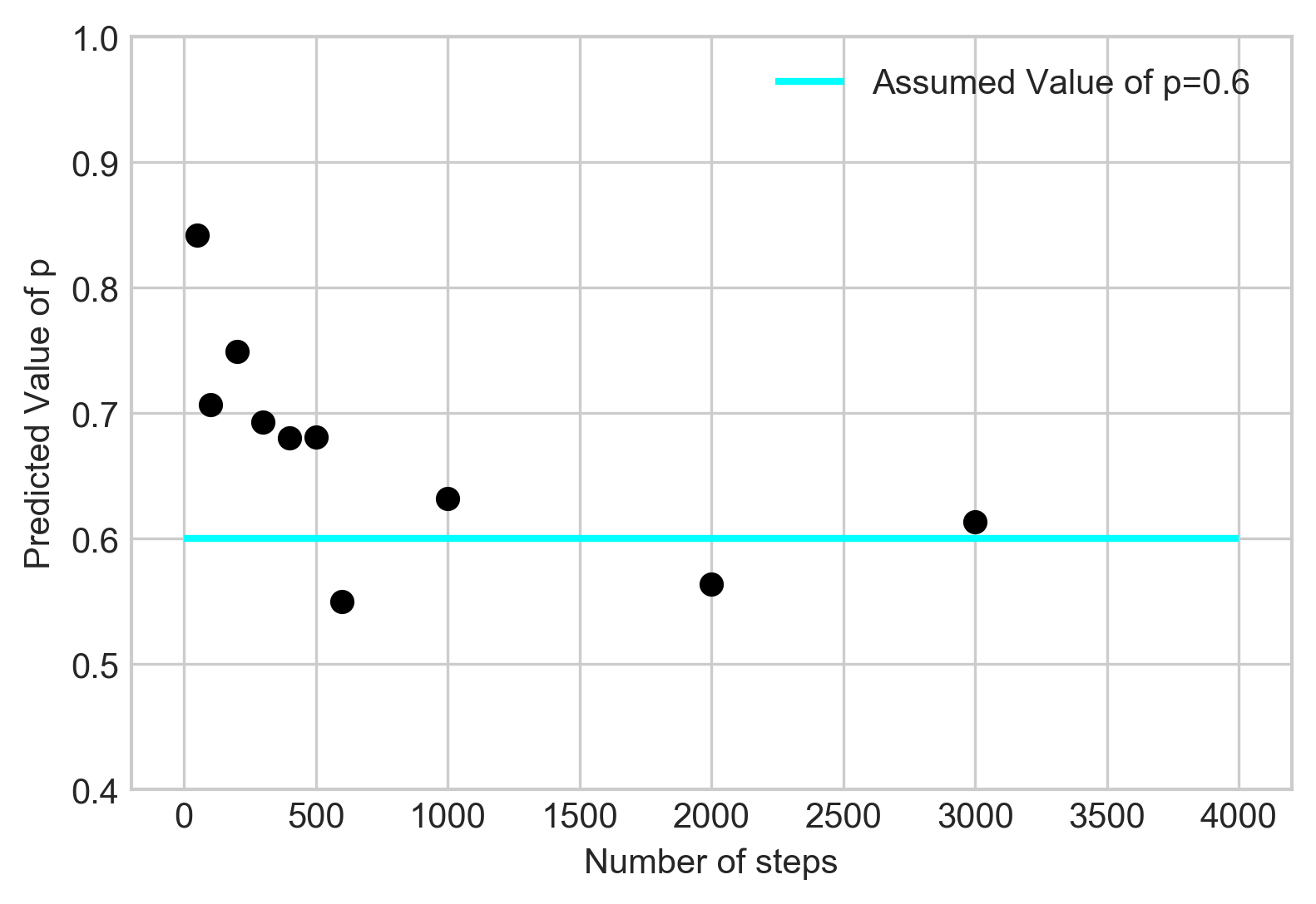
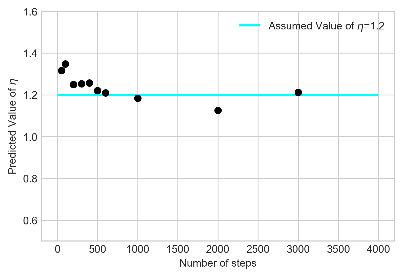
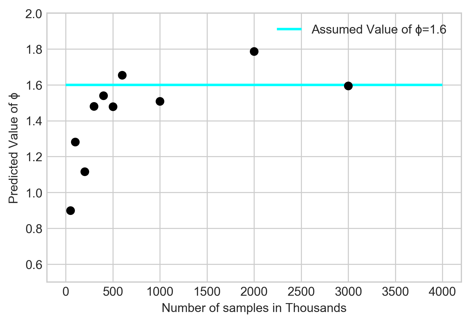
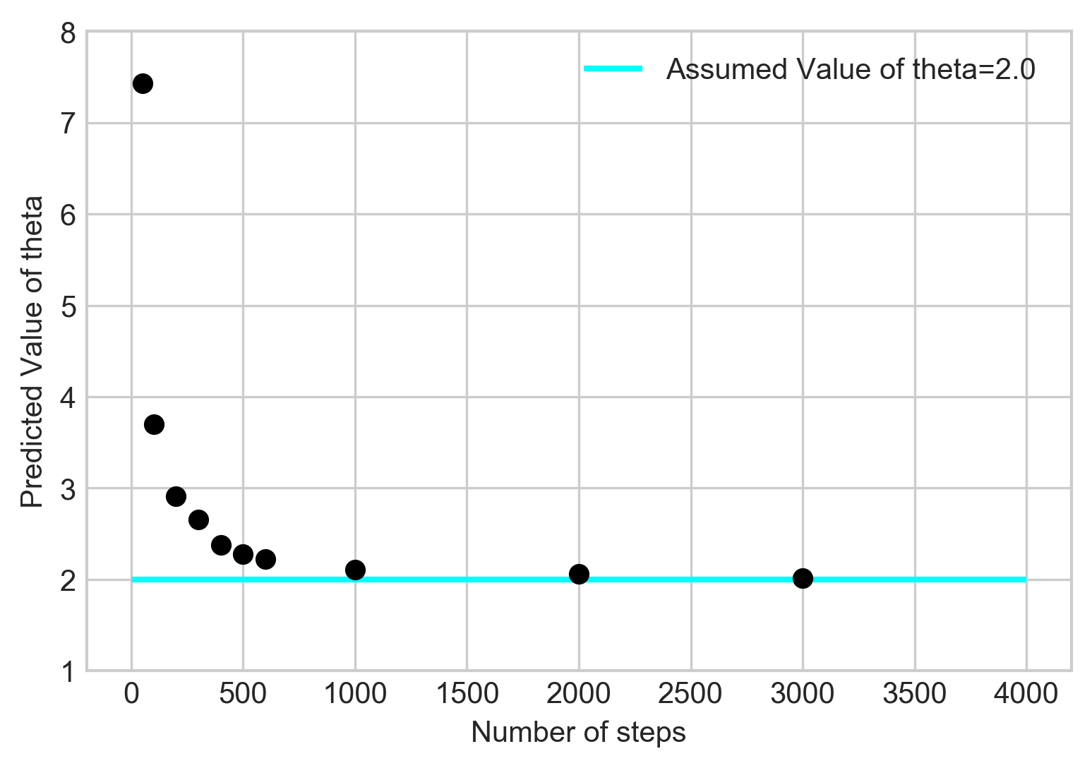
To validate our estimators discussed in Section 4, we perform some numerical simulations. We choose the values of p=0.6p=0.6, η=1.2\eta=1.2, φ=1.6\varphi=1.6 and θ=2.0\theta=2.0 (and λ=σ=1{\lambda}={\sigma}=1). With these parameters, we simulate the double exponential Ornstein-Uhlenbeck process using the exact decomposition algorithm given by (5.52). A simulated sample is displayed in Figure 1. Figures 2 and 3 plot the assumed values versus the values by the ergodic estimators. Table 1 lists the approximation of ergodic estimators to the true parameters as the time becomes larger. It demonstrates that the rate of convergence is quite faster.

Refer to caption
Figure 1. Simulated sample path for a double exponential Orntein-Uhlenbeck process with T=20, N=50, h=0.02 η=1.2\eta=1.2, φ=1.6\varphi=1.6 and θ=2.0\theta=2.0, σ=λ=1\sigma=\lambda=1

The table 1 shows the estimated values of the parameters pp, η\eta, ϕ\phi and θ\theta with different number of steps N and fixed h=0.02h=0.02 and T=N​hT=Nh

Refer to caption
(a) Estimated Values of p
Refer to caption
(b) Estimated Values of η\eta
Figure 2. Assumed versus estimated values
Refer to caption
(a) Estimated Values of φ\varphi
Refer to caption
(b) Estimated Values of θ\theta
Figure 3. Assumed versus estimated values
Time Number of steps p=0.6p=0.6 η=1.2\eta=1.2 ϕ=1.6\phi=1.6 θ=2.0\theta=2.0
1 50 0.8421 1.31677 0.8995 7.4297
2 100 0.7070 1.3477 1.2816 3.6995
4 200 0.74925 1.2498 1.1164 2.9127
6 300 0.6928 1.2532 1.4803 2.6587
8 400 0.6804 1.2571 1.5397 2.3808
10 500 0.6812 1.2204 1.4793 2.2743
12 600 0.5500 1.2089 1.6546 2.2217
20 1000 0.6320 1.1836 1.5078 2.1066
40 2000 0.5635 1.1255 1.7866 2.0631
60 3000 0.6135 1.2112 1.5940 2.0128
Table 1. Assumed Values and Estimated values of the parameters with different number of steps N and fixed h=0.02h=0.02 and T=N​hT=Nh

7. Appendix: Covariance matrix AA

In this section we give the expression of the covariance matrix AA in Lemma 4.1. It is very sophisticated to express the entries of this matrix in terms of the parameters of the equation (2.4). So, we keep them as expression of the invariant probability measure of 𝕏0\mathbb{X}_{0} and that of 𝕏k​h\mathbb{X}_{kh}. First, we compute σg1​g1\sigma_{g_{1}g_{1}}.

σg1​g1=Cov​(𝕏0,𝕏0)+2​∑j=1∞[Cov​(𝕏0,𝕏j​h)]=𝔼⁡(𝕏o2)−𝔼​(𝕏o)2+2​∑j=1∞[𝔼⁡(𝕏o​𝕏j​h)−𝔼⁡(𝕏o)​𝔼​(𝕏j​h)]=𝔼⁡(𝕏o2)−𝔼​(𝕏o)2+2​∑j=1∞[𝔼⁡(𝕏o​𝕏j​h)−[𝔼⁡(𝕏o)]2],\begin{split}\sigma_{g_{1}g_{1}}&=\hbox{Cov}(\mathbb{X}_{0},\mathbb{X}_{0})+2\sum_{j=1}^{\infty}[\hbox{Cov}(\mathbb{X}_{0},\mathbb{X}_{jh})]\\ &=\mathbb{E}(\mathbb{X}_{o}^{2})-\mathbb{E}(\mathbb{X}_{o})^{2}+2\sum_{j=1}^{\infty}\Big[\mathbb{E}(\mathbb{X}_{o}{\mathbb{X}_{jh}})-\mathbb{E}(\mathbb{X}_{o})\mathbb{E}({\mathbb{X}_{jh}})\Big]\\ &=\mathbb{E}(\mathbb{X}_{o}^{2})-\mathbb{E}(\mathbb{X}_{o})^{2}+2\sum_{j=1}^{\infty}\Big[\mathbb{E}(\mathbb{X}_{o}{\mathbb{X}_{jh}})-\left[\mathbb{E}(\mathbb{X}_{o})\right]^{2}\Big]\,,\end{split} (7.53)

where we used 𝔼⁡(𝕏j​h)=𝔼⁡(𝕏0)\mathbb{E}({\mathbb{X}_{jh}})=\mathbb{E}({\mathbb{X}_{0}}). Now we compute σg2​g2\sigma_{g_{2}g_{2}}.

σg2​g2=Cov​(𝕏02,𝕏02)+2​∑j=1∞[Cov​(𝕏02,𝕏j​h2)]=𝔼⁡(𝕏o4)−𝔼​(𝕏o2)2+2​∑j=1∞[𝔼⁡(𝕏o2​𝕏j​h2)−𝔼​(𝕏o2)2].\begin{split}\sigma_{g_{2}g_{2}}&=\hbox{Cov}(\mathbb{X}_{0}^{2},\mathbb{X}_{0}^{2})+2\sum_{j=1}^{\infty}[\hbox{Cov}(\mathbb{X}_{0}^{2},\mathbb{X}_{jh}^{2})]\\ &=\mathbb{E}(\mathbb{X}_{o}^{4})-\mathbb{E}(\mathbb{X}_{o}^{2})^{2}+2\sum_{j=1}^{\infty}\Big[\mathbb{E}(\mathbb{X}_{o}^{2}{\mathbb{X}_{jh}}^{2})-\mathbb{E}(\mathbb{X}_{o}^{2})^{2}\Big]\,.\end{split} (7.54)

Similarly, we have

σg3​g3=Cov​(𝕏03,𝕏03)+2​∑j=1∞[Cov​(𝕏03,𝕏j​h3)]=𝔼⁡(𝕏o6)−𝔼​(𝕏o3)2+2​∑j=1∞[𝔼⁡(𝕏o3​𝕏j​h3)−𝔼​(𝕏o3)2]\begin{split}\sigma_{g_{3}g_{3}}&=\hbox{Cov}(\mathbb{X}_{0}^{3},\mathbb{X}_{0}^{3})+2\sum_{j=1}^{\infty}[\hbox{Cov}(\mathbb{X}_{0}^{3},\mathbb{X}_{jh}^{3})]\\ &=\mathbb{E}(\mathbb{X}_{o}^{6})-\mathbb{E}(\mathbb{X}_{o}^{3})^{2}+2\sum_{j=1}^{\infty}\Big[\mathbb{E}(\mathbb{X}_{o}^{3}{\mathbb{X}_{jh}}^{3})-\mathbb{E}(\mathbb{X}_{o}^{3})^{2}\Big]\end{split} (7.55)

and

σg4​g4=Cov​(𝕏0​𝕏h,𝕏0​𝕏h)+2​∑j=1∞[Cov​(𝕏0​𝕏h,𝕏j​h​𝕏(j+1)​h)]=𝔼⁡((𝕏0​𝕏h)2)−𝔼​(𝕏0​𝕏h)2+2∑j=1∞[𝔼(𝕏0𝕏h𝕏j​h𝕏(j+1)​h)−𝔼(𝕏0𝕏h)𝔼(𝕏j​h𝕏(j+1)​h)].\begin{split}\sigma_{g_{4}g_{4}}&=\hbox{Cov}(\mathbb{X}_{0}\mathbb{X}_{h},\mathbb{X}_{0}\mathbb{X}_{h})+2\sum_{j=1}^{\infty}[\hbox{Cov}(\mathbb{X}_{0}\mathbb{X}_{h},\mathbb{X}_{jh}\mathbb{X}_{(j+1)h})]\\ &=\mathbb{E}((\mathbb{X}_{0}\mathbb{X}_{h})^{2})-\mathbb{E}(\mathbb{X}_{0}\mathbb{X}_{h})^{2}\\ &\qquad+2\sum_{j=1}^{\infty}\Big[\mathbb{E}(\mathbb{X}_{0}\mathbb{X}_{h}\mathbb{X}_{jh}\mathbb{X}_{(j+1)h})-\mathbb{E}(\mathbb{X}_{0}\mathbb{X}_{h})\mathbb{E}(\mathbb{X}_{jh}\mathbb{X}_{(j+1)h})\Big]\,.\end{split} (7.56)

σg1​g2\sigma_{g_{1}g_{2}} is computed as follows.

σg1​g2=Cov​(𝕏0,𝕏02)+∑j=1∞[Cov​(𝕏0,𝕏j​h2)+Cov​(𝕏02,𝕏j​h)]=𝔼((𝕏0)3)−𝔼(𝕏0)𝔼(𝕏02)+∑j=1∞[𝔼(𝕏0𝕏j​h2)−𝔼(𝕏0)𝔼(𝕏j​h2)+𝔼(𝕏02𝕏j​h)−𝔼(𝕏02)𝔼(𝕏j​h)].\begin{split}\sigma_{g_{1}g_{2}}&=\hbox{Cov}(\mathbb{X}_{0},\mathbb{X}_{0}^{2})+\sum_{j=1}^{\infty}[\hbox{Cov}(\mathbb{X}_{0},\mathbb{X}_{jh}^{2})+\hbox{Cov}(\mathbb{X}_{0}^{2},\mathbb{X}_{jh})]\\ &=\mathbb{E}((\mathbb{X}_{0})^{3})-\mathbb{E}(\mathbb{X}_{0})\mathbb{E}(\mathbb{X}_{0}^{2})+\sum_{j=1}^{\infty}\Big[\mathbb{E}(\mathbb{X}_{0}\mathbb{X}_{jh}^{2})-\mathbb{E}(\mathbb{X}_{0})\mathbb{E}(\mathbb{X}_{jh}^{2})\\ &+\mathbb{E}(\mathbb{X}_{0}^{2}\mathbb{X}_{jh})-\mathbb{E}(\mathbb{X}_{0}^{2})\mathbb{E}(\mathbb{X}_{jh})\Big]\,.\end{split} (7.57)

In similar way we can get

σg1​g3=Cov​(𝕏0,𝕏03)+∑j=1∞[Cov​(𝕏0,𝕏j​h3)+Cov​(𝕏03,𝕏j​h)]=𝔼((𝕏0)4)−𝔼(𝕏0)𝔼(𝕏03)+∑j=1∞[𝔼(𝕏0𝕏j​h3)−𝔼(𝕏0)𝔼(𝕏j​h3)+𝔼(𝕏03𝕏j​h)−𝔼(𝕏03)𝔼(𝕏j​h)]\begin{split}\sigma_{g_{1}g_{3}}&=\hbox{Cov}(\mathbb{X}_{0},\mathbb{X}_{0}^{3})+\sum_{j=1}^{\infty}[\hbox{Cov}(\mathbb{X}_{0},\mathbb{X}_{jh}^{3})+\hbox{Cov}(\mathbb{X}_{0}^{3},\mathbb{X}_{jh})]\\ &=\mathbb{E}((\mathbb{X}_{0})^{4})-\mathbb{E}(\mathbb{X}_{0})\mathbb{E}(\mathbb{X}_{0}^{3})+\sum_{j=1}^{\infty}\Big[\mathbb{E}(\mathbb{X}_{0}\mathbb{X}_{jh}^{3})-\mathbb{E}(\mathbb{X}_{0})\mathbb{E}(\mathbb{X}_{jh}^{3})\\ &+\mathbb{E}(\mathbb{X}_{0}^{3}\mathbb{X}_{jh})-\mathbb{E}(\mathbb{X}_{0}^{3})\mathbb{E}(\mathbb{X}_{jh})\Big]\end{split} (7.58)

and

σg1​g4=Cov​(𝕏0,𝕏0​𝕏h)+∑j=1∞[Cov​(𝕏0,𝕏j​h​𝕏(j+1)​h)+Cov​(𝕏j​h,𝕏0​𝕏h)]=𝔼(𝕏02𝕏h)−𝔼(𝕏0)𝔼(𝕏0𝕏h)+∑j=1∞[𝔼(𝕏0𝕏j​h𝕏(j+1)​h)−𝔼(𝕏0)𝔼(𝕏j​h𝕏(j+1)​h)+𝔼(𝕏0𝕏h𝕏j​h)−𝔼(𝕏j​h)𝔼(𝕏0𝕏h)].\begin{split}\sigma_{g_{1}g_{4}}&=\hbox{Cov}(\mathbb{X}_{0},\mathbb{X}_{0}\mathbb{X}_{h})+\sum_{j=1}^{\infty}[\hbox{Cov}(\mathbb{X}_{0},\mathbb{X}_{jh}\mathbb{X}_{(j+1)h})+\hbox{Cov}(\mathbb{X}_{jh},\mathbb{X}_{0}\mathbb{X}_{h})]\\ &=\mathbb{E}(\mathbb{X}_{0}^{2}\mathbb{X}_{h})-\mathbb{E}(\mathbb{X}_{0})\mathbb{E}(\mathbb{X}_{0}\mathbb{X}_{h})+\sum_{j=1}^{\infty}\Big[\mathbb{E}(\mathbb{X}_{0}\mathbb{X}_{jh}\mathbb{X}_{(j+1)h})-\mathbb{E}(\mathbb{X}_{0})\mathbb{E}(\mathbb{X}_{jh}\mathbb{X}_{(j+1)h})\\ &+\mathbb{E}(\mathbb{X}_{0}\mathbb{X}_{h}\mathbb{X}_{jh})-\mathbb{E}(\mathbb{X}_{jh})\mathbb{E}(\mathbb{X}_{0}\mathbb{X}_{h})\Big]\,.\end{split} (7.59)

σg2​g3\sigma_{g_{2}g_{3}} is similar to σg1​g2\sigma_{g_{1}g_{2}}.

σg2​g3=Cov​(𝕏02,𝕏03)+∑j=1∞[Cov​(𝕏02,𝕏j​h3)+Cov​(𝕏03,𝕏j​h2)]=𝔼((𝕏0)5)−𝔼(𝕏02)𝔼(𝕏03)+∑j=1∞[𝔼(𝕏02𝕏j​h3)−𝔼(𝕏02)𝔼(𝕏j​h3)+𝔼(𝕏03𝕏j​h2)−𝔼(𝕏03)𝔼(𝕏j​h2)].\begin{split}\sigma_{g_{2}g_{3}}&=\hbox{Cov}(\mathbb{X}_{0}^{2},\mathbb{X}_{0}^{3})+\sum_{j=1}^{\infty}[\hbox{Cov}(\mathbb{X}_{0}^{2},\mathbb{X}_{jh}^{3})+\hbox{Cov}(\mathbb{X}_{0}^{3},\mathbb{X}_{jh}^{2})]\\ &=\mathbb{E}((\mathbb{X}_{0})^{5})-\mathbb{E}(\mathbb{X}_{0}^{2})\mathbb{E}(\mathbb{X}_{0}^{3})+\sum_{j=1}^{\infty}\Big[\mathbb{E}(\mathbb{X}_{0}^{2}\mathbb{X}_{jh}^{3})-\mathbb{E}(\mathbb{X}_{0}^{2})\mathbb{E}(\mathbb{X}_{jh}^{3})\\ &+\mathbb{E}(\mathbb{X}_{0}^{3}\mathbb{X}_{jh}^{2})-\mathbb{E}(\mathbb{X}_{0}^{3})\mathbb{E}(\mathbb{X}_{jh}^{2})\Big]\,.\end{split} (7.60)

Finally, we have

σg2​g4=Cov​(𝕏02,𝕏0​𝕏h)+∑j=1∞[Cov​(𝕏02,𝕏j​h​𝕏(j+1)​h)+Cov​((𝕏j​h)2,𝕏0​𝕏h)]=𝔼(𝕏03𝕏h)−𝔼(𝕏02)𝔼(𝕏0𝕏h)+∑j=1∞[𝔼(𝕏02𝕏j​h𝕏(j+1)​h)−𝔼(𝕏02)𝔼((𝕏j​h𝕏(j+1)​h)+𝔼(𝕏0𝕏h𝕏j​h2)−𝔼(𝕏j​h2)𝔼(𝕏0𝕏h)]\begin{split}\sigma_{g_{2}g_{4}}&=\hbox{Cov}(\mathbb{X}_{0}^{2},\mathbb{X}_{0}\mathbb{X}_{h})+\sum_{j=1}^{\infty}[\hbox{Cov}(\mathbb{X}_{0}^{2},\mathbb{X}_{jh}\mathbb{X}_{(j+1)h})+\hbox{Cov}((\mathbb{X}_{jh})^{2},\mathbb{X}_{0}\mathbb{X}_{h})]\\ &=\mathbb{E}(\mathbb{X}_{0}^{3}\mathbb{X}_{h})-\mathbb{E}(\mathbb{X}_{0}^{2})\mathbb{E}(\mathbb{X}_{0}\mathbb{X}_{h})+\sum_{j=1}^{\infty}\Big[\mathbb{E}(\mathbb{X}_{0}^{2}\mathbb{X}_{jh}\mathbb{X}_{(j+1)h})-\mathbb{E}(\mathbb{X}_{0}^{2})\mathbb{E}((\mathbb{X}_{jh}\mathbb{X}_{(j+1)h})\\ &+\mathbb{E}(\mathbb{X}_{0}\mathbb{X}_{h}\mathbb{X}_{jh}^{2})-\mathbb{E}(\mathbb{X}_{jh}^{2})\mathbb{E}(\mathbb{X}_{0}\mathbb{X}_{h})\Big]\end{split} (7.61)

and

σg3​g4=Cov​(𝕏03,𝕏0​𝕏h)+∑j=1∞[Cov​(𝕏03,𝕏j​h​𝕏(j+1)​h)+Cov​((𝕏j​h)3,𝕏0​𝕏h)]=𝔼(𝕏04𝕏h)−𝔼(𝕏03)𝔼(𝕏0𝕏h)+∑j=1∞[𝔼(𝕏03𝕏j​h𝕏(j+1)​h)−𝔼(𝕏03)𝔼((𝕏j​h𝕏(j+1)​h)+𝔼(𝕏0𝕏h𝕏j​h3)−𝔼(𝕏j​h3)𝔼(𝕏0𝕏h)].\begin{split}\sigma_{g_{3}g_{4}}&=\hbox{Cov}(\mathbb{X}_{0}^{3},\mathbb{X}_{0}\mathbb{X}_{h})+\sum_{j=1}^{\infty}[\hbox{Cov}(\mathbb{X}_{0}^{3},\mathbb{X}_{jh}\mathbb{X}_{(j+1)h})+\hbox{Cov}((\mathbb{X}_{jh})^{3},\mathbb{X}_{0}\mathbb{X}_{h})]\\ &=\mathbb{E}(\mathbb{X}_{0}^{4}\mathbb{X}_{h})-\mathbb{E}(\mathbb{X}_{0}^{3})\mathbb{E}(\mathbb{X}_{0}\mathbb{X}_{h})+\sum_{j=1}^{\infty}\Big[\mathbb{E}(\mathbb{X}_{0}^{3}\mathbb{X}_{jh}\mathbb{X}_{(j+1)h})-\mathbb{E}(\mathbb{X}_{0}^{3})\mathbb{E}((\mathbb{X}_{jh}\mathbb{X}_{(j+1)h})\\ &+\mathbb{E}(\mathbb{X}_{0}\mathbb{X}_{h}\mathbb{X}_{jh}^{3})-\mathbb{E}(\mathbb{X}_{jh}^{3})\mathbb{E}(\mathbb{X}_{0}\mathbb{X}_{h})\Big]\,.\end{split} (7.62)

References

  • [1] Billingsley, P. Probability and measure. Anniversary edition. With a foreword by Steve Lalley and a brief biography of Billingsley by Steve Koppes. Wiley Series in Probability and Statistics. John Wiley & Sons, Inc., Hoboken, NJ, 2012.
  • [2] Billingsley, P. Statistical inference for Markov processes. Statistical Research Monographs, Vol. II. The University of Chicago Press, Chicago, Ill. 1961.
  • [3] Cai, N.; Chen, N. and Wan, X. Occupation times of jump-diffusion processes with double exponential jumps and the pricing of options. Math. Oper. Res. 35 (2010), no. 2, 412-437.
  • [4] Hackmann, D. Analytic techniques for option pricing under a hyperexponential Lévy model. J. Comput. Appl. Math. 342 (2018), 225–248.
  • [5] Cheng, Y., Hu, Y. and Long, H. Generalized moment estimators for α\alpha-stable Ornstein-Uhlenbeck motions from discrete observations. Stat. Inference Stoch. Process. 23 (2020), no. 1, 53-81.
  • [6] Haress, E. M. and Hu, Y. Estimation of all parameters in the fractional Ornstein-Uhlenbeck model under discrete observations. Stat. Inference Stoch. Process. 24 (2021), no. 2, 327-351.
  • [7] Jones, G. L. On the Markov chain central limit theorem. Probab. Surv. 1 (2004), 299-320.
  • [8] Lukacs, E. Characteristic functions. Second edition, revised and enlarged. Hafner Publishing Co., New York, 1970.
  • [9] Qu, Y., A. Dassios, and H. Zhao. Exact Simulation of Gamma-driven Ornstein–Uhlenbeck Processes with Finite and Infinite Activity Jumps. Journal of the Operational Research Society, 2019: 1–14.
  • [10] Jongbloed, G.; van der Meulen, F. H.; van der Vaart, A. W. Nonparametric inference for Lévy-driven Ornstein-Uhlenbeck processes. Bernoulli 11 (2005), no. 5, 759-791.
  • [11] Masuda, H. Ergodicity and exponential β\beta-mixing bounds for multidimensional diffusions with jumps. Stochastic Process. Appl. 117 (2007), no. 1, 35-56.
  • [12] Dellacherie, C. and Meyer, P. A. Probabilities and potential. North-Holland Mathematics Studies, 29. North-Holland Publishing Co., Amsterdam-New York, 1978.
  • [13] Ibragimov, I. A.; Linnik, Yu. V. Independent and stationary sequences of random variables. Wolters-Noordhoff Publishing, Groningen, 1971.
  • [14] Sato, K. Lévy processes and infinitely divisible distributions. Cambridge Studies in Advanced Mathematics, 68. Cambridge University Press, Cambridge, 2013.
  • [15] Meyn S.P and Tweedie R.L. Stability of Markovian processes. II.Continuous-time processes and sampled chains. Adv. in Appl. Probab., 25(3):487-517, 1993.