Low-to-Zero-Overhead IRS Reconfiguration: Decoupling Illumination and Channel EstimationThanks: V. Jamali and H. Vincent Poor are with the Department of Electrical and Computer Engineering, Princeton University, Princeton, NJ 08544 USA (e-mail: {jamali, poor}@princeton.edu).Thanks: G. C. Alexandropoulos is with the Department of Informatics and Telecommunications, National and Kapodistrian University of Athens, Panepistimiopolis Ilissia, 15784 Athens, Greece. (e-mail: alexandg@di.uoa.gr).Thanks: R. Schober is with the Institute for Digital Communications at Friedrich-Alexander University Erlangen-Nürnberg (FAU), Erlangen, Germany (e-mail: robert.schober@fau.de).
Abstract
Most algorithms developed for the optimization of Intelligent Reflecting Surfaces (IRSs) so far require knowledge of full Channel State Information (CSI). However, the resulting acquisition overhead constitutes a major bottleneck for the realization of IRS-assisted wireless systems in practice. In contrast, in this paper, focusing on downlink transmissions from a Base Station (BS) to a Mobile User (MU) that is located in a blockage region, we propose to optimize the IRS for illumination of the area centered around the MU. Hence, the proposed design requires the estimation of the MU’s position and not the full CSI. For a given IRS phase-shift configuration, the end-to-end BS-IRS-MU channel can then be estimated using conventional channel estimation techniques. The IRS reconfiguration overhead for the proposed scheme depends on the MU mobility as well as on how wide the coverage of the IRS illumination is. Therefore, we develop a general IRS phase-shift design, which is valid for both the near- and far-field regimes and features a parameter for tuning the size of the illumination area. Moreover, we study a special case where the IRS illuminates the entire blockage area, which implies that the IRS phase shifts do not change over time leading to zero overhead for IRS reconfiguration.
Index Terms:
Intelligent reflecting surfaces, channel estimation, blockage area, illumination area, low-overhead design.I Introduction
Intelligent Reflecting Surfaces (IRSs) have attracted significant attention as an enabling technology for the realization of smart radio environments in future sixth generation (6G) wireless systems [1, 2]. However, the envisioned performance gain of IRSs mostly relies on the availability of Channel State Information (CSI), which given the typically large number of reflecting elements, denoted henceforth by , translates into a huge, often unaffordable, CSI acquisition overhead [3, 4].
Various channel estimation techniques have been proposed in the literature; see [3] for a recent overview. For example, the ON/OFF protocol proposed in [5] comprises stages, where in each stage, only one reflecting element is ON and the corresponding cascaded Base Station (BS)-IRS-Mobile User (MU) channel is estimated. To improve the estimation accuracy, a Discrete Fourier Transform (DFT) based protocol was proposed in [6] which again employs stages but, in each stage, all IRS elements are ON and their reflection coefficients are designed based on one of the columns of the DFT matrix. In [7], the authors proposed an algorithm which estimates the BS-IRS and IRS-MU channels on two different time scales. In particular, they exploited the fact that the BS-IRS channel changes much more slowly than the IRS-MU channel, since the IRS and the BS are fixed nodes and the IRS is often deployed to ensure a Line-of-Sight (LoS) BS-IRS link. Nonetheless, the overhead of all of these channel estimation techniques scales with , which hinders their application for practically large IRSs.
Two categories of IRS channel estimation schemes have been proposed in the literature whose overhead does not scale with , namely sparsity- and codebook-based schemes [8, 9]. In particular, the sparsity of the wireless channel in the angular domain was exploited in [8] to design a channel estimation algorithm. Therefore, the corresponding overhead scales with the number of dominant propagation paths of the wireless channel. In contrast, in [9], the authors proposed to estimate the end-to-end BS-IRS-MU channel only for a limited number of IRS phase-shift configurations drawn from a codebook. Since the channel estimation overhead scales with the codebook size, an IRS phase-shift profile was developed, which allows the design of small-size phase-shift codebooks.
Regardless of which of the above CSI acquisition schemes is adopted, the common drawback of optimizing the IRS based on CSI is that, since channel gains change quickly, the IRS should be in principle frequently reconfigured (e.g., typical channel coherence times are on the order of milliseconds [10]). In contrast, in this paper, we propose to decouple the IRS reconfiguration from channel estimation. We focus on downlink transmissions from a BS to an MU that is located in a blockage region. The basic idea behind the proposed scheme is that the IRS is configured to illuminate the MU and is only reconfigured if the MU’s Quality-of-Service (QoS) requirement cannot be met. Hence, the frequency of IRS reconfiguration does not explicitly depend on the channel coherence time, but on the mobility of the user, the size of the area illuminated by the IRS, and the MU QoS requirement. Once the IRS is configured, it acts as a virtual channel scatterer and the end-to-end BS-IRS-MU channel can be estimated based on conventional channel estimation techniques, and with a frequency that is dictated by the channel coherence time [11]. To facilitate the proposed approach, we develop a general IRS phase-shift design, which unlike those in [9, 12] is valid for both the near- and far-field regimes and features a parameter for tuning the size of the illuminated area. We analyze the corresponding overhead and compare it with that of the existing schemes. Moreover, we study an interesting special case where the IRS illuminates the entire blockage area, avoiding the need for IRS reconfiguration.
II Communication Setup
II-A System Model
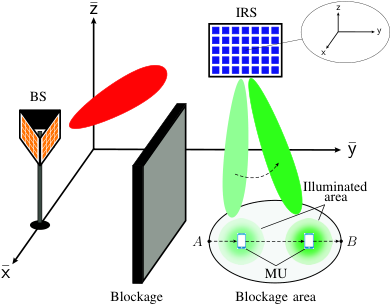
We consider a downlink system, where a multi-antenna BS wishes to serve a single-antenna MU. We assume that there exists an area where direct coverage is not available due to, e.g., the presence of a blocking building, see Fig. 1. To address this issue, an IRS is deployed such that it has a LoS connection to both the BS and the MU, enabling the realization of a virtual non-LoS link between the BS and the MU. Since the BS and IRS are fixed nodes, we assume that the BS employs a fixed active beamformer directed towards the IRS. Hence, the equivalent baseband signal model is given by [4]
| (1) |
where , , and denote the BS’s data symbol, the MU’s received signal, and the additive white Gaussian noise at the MU with zero mean and variance , respectively. Moreover, denotes the effective channel coefficient (including the impact of BS beamforming) between the BS and the -th reflecting element of the IRS, and denotes the channel coefficient between the -th reflecting element of the IRS and the single MU antenna. Furthermore, is the reflection coefficient of the -th IRS reflecting element, where and are the amplitude and phase of , respectively.
II-B Scattering Integral
While the received signal model in (1) is useful for characterizing the system on the small discrete-time scale, it is too general and abstract for an insightful design and performance analysis of the IRS. To cope with this issue, in this paper, we base our design on the LoS links, which for small sub-wavelength IRS element spacing, can be accurately characterized by the scattering integral [4, Fig. 4]. In particular, using the scalar representation of this integral, the reflected electric field at MU position can be derived as [13]
| (2) |
where and are the amplitude and phase, respectively, of the incident wave at point on the IRS; is the ratio of reflected and incident electric fields (i.e., field reflection coefficient) where is the phase shift applied by IRS at point and is a constant that ensures the passivity of the IRS, which in general depends on the incident and reflection angles [4, Remark 1]. and denote the IRS dimension along the - and -axes, respectively; and represent the wavelength and wave number, respectively.
For completeness, we show in [14, Appendix], which is an extended version of this letter, that the abstract model in (1) is a consistent approximation of the physical model in (2) for a lossless IRS (i.e., ), when assuming that and comprise only LoS links in an unobstructed propagation medium. For this case, the channel coeffitients are chosen as and , respectively, where and denote the directivity of the BS and MU antennas, respectively; denotes the effective power gain factor of each IRS element having area ; and are the distances between the BS and MU to the center of the IRS, respectively; and and denote the distances between the BS and MU to the -th IRS unit cell, respectively.
Neglecting the noise, the transmit and received symbol powers and , respectively, defined based on (1), can be obtained from (2) by relating the electric fields and power densities in space according to [4, Appendix A]:
| (3) |
where represents the free-space characteristic impedance. We next employ (1) for channel estimation and (2) for IRS phase-shift design.
II-C User Mobility Model
Depending on the application of interest, various user mobility models have been proposed in the literature; see [15] for an overview. In this paper, we adopt a simple user mobility model, which is a special case of the random waypoint mobility model [15]. We specifically assume that the MU enters and leaves the area at random points and , respectively, in Fig. 1, and crosses the area on a straight line with a fixed velocity .
III Low-overhead IRS Reconfiguration
III-A Proposed Algorithm
The proposed IRS reconfiguration and channel estimation algorithm consists of the following three sub-blocks:
Sub-block 1 (MU Localization): Recall that the IRS is deployed to have LoS connections to both the BS and the MU. Since the IRS and BS are fixed nodes, their relative positions can be estimated once, and then, considered as known. However, the position of the MU, denoted by , varies due to its mobility which can be estimated using existing localization algorithms (see, e.g., [16, 17]). Note that if the MU is in the far field of the IRS, it suffices for this localization sub-block to estimate the Angle-of-Departure (AoD) from the IRS to the MU.
Sub-block 2 (IRS Phase-Shift Design): We assume that the IRS phase-shift design is based only on the MU position or the required AoD in the case of far field. However, the IRS radiation pattern can be designed to be narrow [4] or wide [9, 12], depending on the IRS configuration objective. This will be discussed in detail in the following Section III-B.
Sub-block 3 (End-to-End Channel Estimation): Once the IRS is configured, the BS and the MU treat the surface as a part of the end-to-end wireless channel , which can be estimated using standard (e.g., Least Squares (LS)) channel estimation techniques [11].
Figure 2 illustrates how the above three sub-blocks are employed in the proposed communication protocol, where denotes the time duration needed by the adopted localization algorithm to estimate/update the MU’s position; is the time duration needed to compute the IRS phase shifts and/or inform the IRS; represents the time duration needed by the adopted channel estimation algorithm to estimate the end-to-end channel; denotes the channel coherence time; and is the time duration between two consecutive configurations of the IRS. We assume that the IRS is updated (using sub-blocks 1 and 2) once the current IRS illumination pattern cannot support the MU’s QoS any more. Thereby, we consider that the MU continuously calculates the average Signal-to-Noise Ratio (SNR) (for which the fading is averaged out, and hence, it is determined by the LoS link), and once it falls below a certain threshold, denoted by , the MU sends a feedback message to the BS to initiate the MU localization and IRS phase-shift update. The proposed IRS configuration and channel estimation algorithm is summarized in Algorithm 1, where is a parameter that controls the size of the illuminated area, as will be explained in the next subsection.
input: Illumination parameter and SNR requirement .
output: Update of MU position , IRS phase shifts , , and end-to-end channel .
III-B IRS Phase-Shift Design
Since various IRS-assisted localization schemes [16, 17] and conventional channel estimation schemes [11] have been proposed in the literature, in this section, we focus our attention on the design and analysis of efficient IRS phase-shift configurations enabling narrow and wide illuminations, respectively.
III-B1 Beam Focusing
In order to maximize the power at the MU position (i.e., maximize via (2)), the following phase shift needs to be applied at point on the IRS:
| (4) |
Substituting the above IRS phase shifts in (2) and then in the expression in (3) yields the maximum average SNR:
| (5) |
where denotes the distance between the IRS center and the MU, and we used to approximate the amplitude in (2). The main parameter that determines the overhead of the proposed design is how the SNR decays around the focus point, which is numerically evaluated in the top subfigure in Fig. 3 for an example scenario. As can be observed from this figure, for this setup with the SNR requirement of dB, the coverage size along the - and -directions around the focus point are m and m ( m and m), respectively, for GHz ( GHz) carrier frequency. Hence, we can conclude that, for typical walking speeds of approximately m/s [15], the IRS update time is on the order of seconds, which is orders of magnitude larger than typical channel coherence times; those times are on the order of milliseconds [10].
III-B2 Wide Illumination
In order to further reduce the IRS reconfiguration overhead, we propose to widen the reflected beam around the MU’s location to increase the area in which the SNR is above the required threshold . Let , , and denote the sets of points on the IRS, the blockage area, and the area that we wish to illuminate by the IRS, respectively. Suppose that if the IRS is set for full focusing based on (4), only a fraction of the targeted area is illuminated. To illuminate the entire desired area, we partition the IRS into sub-surfaces and split the targeted illumination area into sub-regions, where each sub-surface on the IRS illuminates the center of one sub-region. A general formulation of this problem is a mapping from each point on the IRS to one of the sub-regions in the targeted illumination area. Let denote the set containing the centers of the sub-regions. Given this mapping, the corresponding IRS phase shift for wide illumination, denoted by , , can be obtained as a function of in (4), as follows:
| (6) |
The term is the reference distance from each point to the IRS center, , whose contribution is removed from . Intuitively, even for focusing, the term only contributes to the signal’s phase at the focus point and not to the corresponding power. Since we are mainly interested in the power at the desired observation points within , and not in the phase, the contribution of the reference distances, i.e., , are removed from the phase-shift design in (6).
Next, we discuss our proposed choices of the mapping function and the set . In principle, can be a set of discrete points , but which and how many points to choose are non-trivial tasks. More importantly, for a given discrete set , the illumination patterns of the corresponding sub-regions interfere with each other and may cause severe fluctuations in the received powers particularly at the sub-region boundaries. To circumvent these challenges, we choose a continuous set spanning the entire targeted area, namely . Therefore, becomes a continuous mapping from to , an example of which is provided in the following.
Example 1: Let us assume and a square area for parallel to the plane (i.e., the MU does not change its height). For this case, we propose the following simple mapping from to (needed in (6)):
| (7) |
which leads to the following IRS phase-shift design:
| (8) |
We can see from (7) that by varying point on the IRS, i.e., , the output of the mapping varies and covers the entire targeted area, i.e., . In other words, each part of the IRS locally focuses on one point in the set , and the phase shift across the IRS gradually varies such that all points in are illuminated. The bottom figure of Fig. 3 shows that for carrier frequencies of GHz and GHz using m and m, respectively, the areas supporting SNR threshold dB along -axis are respectively m and m, which implies a reduced IRS reconfiguration overhead compared to beam focusing.
Example 2: Suppose that the BS and MU are in the far-field of the IRS. In this case, the phase shift given by (4) reduces to the following linear phase shift [4]:
| (9) |
where and denote respectively the incident and reflection angles with and for being the elevation and azimuth angles in the IRS spherical coordinate system, respectively; with ; ; and . Note that in the far-field regime, the position can be replaced by the corresponding AoD , where is the set of possible AoDs. For the ease of presentation, we assume that the range translates into the following intervals for and . Here, we propose the following mapping from to (or equivalently to ):
| (10) |
where , , , and . Substituting (9) and (10) into the general IRS phase shift in (6), we obtain the illumination of the desired width:
| (11) |
This phase-shift design is similar to the quadratic phase-shift profile proposed in [9] for the realization of small-sized IRS phase-shift codebooks.
Remark 1
III-B3 Full Illumination
Next, we discuss an interesting special case where the IRS illuminates the entire blockage area and hence no IRS reconfiguration is required, i.e., the IRS reconfiguration overhead is zero. This may be achieved in the phase-shift design proposed in (8) by setting . In the following, we study for which parameter values, the MU’s QoS can be met based on full illumination for an idealized scenario.
Let us assume that the blockage area is larger than what can be covered by focusing, as realized with (4). We assume an idealized IRS illumination where the entire power received by the IRS is uniformly distributed across the blockage area. Note that such illumination cannot be realized by an IRS [4], but it provides a performance upper bound for the proposed IRS phase-shift design. Using (3), this leads to the following SNR across the blockage area:
| (12) |
where and denotes the size of the blockage area. The above expression can be used to characterize the tradeoff between the BS’s transmit power, the IRS size, and the size of the blockage area where the SNR constraint holds across the entire illuminated area.
III-C Overhead Comparison
Table I presents an approximate characterization of the overhead of the proposed IRS reconfiguration and CSI acquisition scheme, and that of several benchmark schemes from the literature for the considered communication system detailed in Section II, in terms of the underlying key parameters. We consider pilot symbols used only for channel estimation and localization, and neglect the time consumed for the feedback of the estimated CSI, MU position, and IRS phase shifts.
For the ON/OFF- and DFT matrix-based methods [5, 6], we assume that in each of the stages, pilot symbols of length are sent. We use the sparsity-based method in [8] jointly with the two timescale-based method in [7], where the overhead of BS-IRS channel estimation is neglected and the number of pilot symbols needed to estimate the IRS-MU channel is assumed to be with and being the number of paths in the IRS-MU link and the number of discrete grid points, respectively, and is a constant that depends on the adopted compressed sensing algorithm. The codebook size for codebook-based channel estimation is denoted by . For the proposed scheme, the value of in general depends on the adopted localization scheme. However, if sparsity-based localization is adopted and the MU’s position is assumed to be along the dominant path, the number of required pilot symbols, and hence, is upper bounded by [8].
IV Simulation Results
The communication setup considered in this section is schematically illustrated in Fig. 1 and the values of the system parameters are identical to those used for Fig. 3 unless otherwise stated. The channel coherence time is computed based on [10, Eq. (8)] and is approximately ms at GHz and m/s. The blockage area is a circle with center and diameter . The illumination scheme in (8) is adopted which reduces to the near-field focusing in (4) for .
In Fig. 4, we plot the overhead of only the IRS reconfiguration and the combined overhead of the IRS reconfiguration and channel estimation for the proposed scheme as a function of the required SNR. Moreover, we include the channel estimation overhead for the different benchmark schemes given in Table I for comparison. The vertical lines in Fig. 4 represent the maximum SNR that is achievable for all points within the blockage area and can be attained only via instantaneous IRS reconfiguration. This figure suggests that, unless the required SNR is extremely close the maximum achievable SNR, the IRS reconfiguration overhead is orders of magnitude less than the channel estimation overhead. In other words, at the cost of a negligible overhead, the proposed scheme can support SNRs which are quite close (e.g., within dB) to the upper bound. Moreover, we observe from Fig. 4 that, compared to near-field focusing (), wide illumination ( m) yields a lower IRS reconfiguration overhead for low required SNR values.
In Fig. 5, we plot the minimum transmit power needed to support dB via full illumination (i.e., zero IRS reconfiguration overhead) as a function of the blockage area diameter. As can be seen from this figure, for near-field focusing, the transmit power has to significantly increase as the blockage area size increases. In contrast, wider illumination requires a smaller transmit power for larger blockage areas. An un-attainable lower bound for the transmit power obtained from (12) and a lower bound achievable by instantaneous focusing (incurring overhead) are also plotted for comparison.
V Conclusions
In this paper, we have shown that the overhead of IRS reconfiguration can be significantly reduced by decoupling it from channel estimation. Thereby, the IRS reconfiguration overhead scales neither with the number of IRS elements nor with the channel coherence time, but it is a function of the MU’s speed, its QoS requirements, and the IRS phase-shift design. Moreover, we have proposed a novel IRS phase-shift design which is valid for both near- and far-field transmission and features a parameter that tunes the width of the illuminated area. An interesting topic for future research is the use of machine learning tools for the localization and prediction of the IRS phase-shift configurations needed in the proposed scheme.
References
- [1] X. Yu, V. Jamali, D. Xu, D. W. K. Ng, and R. Schober, “Smart and reconfigurable wireless communications: From IRS modeling to algorithm design,” IEEE Wireless Commun. Mag., to appear, 2021.
- [2] E. Calvanese Strinati, G. C. Alexandropoulos et al., “Reconfigurable, intelligent, and sustainable wireless environments for 6G smart connectivity,” IEEE Commun. Mag., vol. 59, no. 10, p. 99–105, Oct. 2021.
- [3] L. Wei, C. Huang, G. C. Alexandropoulos, C. Yuen, Z. Zhang, and M. Debbah, “Channel estimation for RIS-empowered multi-user MISO wireless communications,” IEEE Trans. Commun., vol. 69, no. 6, pp. 4144–4157, Jun. 2021.
- [4] M. Najafi, V. Jamali, R. Schober, and H. V. Poor, “Physics-based modeling and scalable optimization of large intelligent reflecting surfaces,” IEEE Trans. Commun., vol. 69, no. 4, pp. 2673–2691, Apr. 2021.
- [5] D. Mishra and H. Johansson, “Channel estimation and low-complexity beamforming design for passive intelligent surface assisted MISO wireless energy transfer,” in Proc. IEEE Int. Conf. Acoustics, Speech, Sig. Process. (ICASSP), 2019, pp. 4659–4663.
- [6] B. Zheng and R. Zhang, “Intelligent reflecting surface-enhanced OFDM: Channel estimation and reflection optimization,” IEEE Wireless Commun. Lett., vol. 9, no. 4, pp. 518–522, 2019.
- [7] C. Hu, L. Dai, S. Han, and X. Wang, “Two-timescale channel estimation for reconfigurable intelligent surface aided wireless communications,” IEEE Trans. Commun., 2021.
- [8] P. Wang, J. Fang, H. Duan, and H. Li, “Compressed channel estimation for intelligent reflecting surface-assisted millimeter wave systems,” IEEE Sig. Process. Lett., vol. 27, pp. 905–909, 2020.
- [9] V. Jamali, M. Najafi, R. Schober, and H. V. Poor, “Power efficiency, overhead, and complexity tradeoff of IRS codebook design–Quadratic phase-shift profile,” IEEE Commun. Lett., vol. 25, no. 6, pp. 2048–2052, Jun. 2021.
- [10] R. P. Torres and J. R. Pérez, “A lower bound for the coherence block length in mobile radio channels,” MDPI Electron., vol. 10, no. 4, p. 398, Feb. 2021.
- [11] L. Liu and W. Yu, “Massive connectivity with massive MIMO–Part I: Device activity detection and channel estimation,” vol. 66, no. 11, pp. 2933–2946, Jun. 2018.
- [12] F. Laue, V. Jamali, and R. Schober, “IRS-assisted active device detection,” in Proc. IEEE Int. Workshop Sig. Process. Advances in Wireless Commun. (SPAWC), 2021, pp. 1–5.
- [13] C. A. Balanis, Antenna Theory: Analysis and Design. John Wiley & Sons, 2015.
- [14] V. Jamali, G. C. Alexandropoulos, R. Schober, and H. V. Poor, “Low-to-zero-overhead IRS reconfiguration: Decoupling illumination and channel estimation (extended version),” arXiv preprint arXiv:2111.09421, 2021.
- [15] Q. Zheng, X. Hong, and S. Ray, “Recent advances in mobility modeling for mobile ad hoc network research,” in Proc. 42nd Annual Southeast Regional Conf., 2004, pp. 70–75.
- [16] H. Wymeersch, J. He, B. Denis, A. Clemente, and M. Juntti, “Radio localization and mapping with reconfigurable intelligent surfaces: Challenges, opportunities, and research directions,” IEEE Veh. Technol. Mag., vol. 15, no. 4, pp. 52–61, Dec. 2020.
- [17] Z. Abu-Shaban, K. Keykhosravi, M. F. Keskin, G. C. Alexandropoulos, G. Seco-Granados, and H. Wymeersch, “Near-field localization with a reconfigurable intelligent surface acting as lens,” in Proc. IEEE Int. Conf. Commun. (ICC), 2021, pp. 1–6.
- [18] M. T. Ivrlač and J. A. Nossek, “Toward a circuit theory of communication,” IEEE Trans. Circuits Syst. I, vol. 57, no. 7, pp. 1663–1683, 2010.
- [19] M. Di Renzo, A. Zappone, M. Debbah, M.-S. Alouini, C. Yuen, J. De Rosny, and S. Tretyakov, “Smart radio environments empowered by reconfigurable intelligent surfaces: How it works, state of research, and the road ahead,” IEEE J. Select. Areas in Commun., vol. 38, no. 11, pp. 2450–2525, 2020.
In this section, we identify the conditions that relate the channel models in (1) and (2). The analysis method is borrowed from [13] and is based on transforming the wave electrical field to the spatial power density using the Poynting theorem, and then, transforming the field power density to the power absorbed/radiated by the receive/transmit antenna given the antenna aperture.
First, we note that the scattering integral in (2) assumes continuous surface approximation, whereas (1) assumes a discrete array model. Therefore, we begin with approximating the integral in (2) by summation where the and axes are discretized with step sizes and , respectively, i.e.,
| (13) | |||||
where approximation is due to discretization with denoting the -th discrete point on the surface. Moreover, approximation is due to the fact that, while we consider the exact distance to compute the phase term , we assume that the variation of the distance can be ignored for the amplitude term , which is a widely-adopted approximation in antenna theory [13]. Here, is the distance from the center of the IRS to the observation point . For , we further define and for simplicity of presentation.
The radiation power intensity (in Watt/m2) at the IRS is obtained as , where is the transmit power, denotes the directivity of the BS antenna, and is the distance between the BS and the center of the IRS. Moreover, for plane waves11 1 While the impinging wave may not be a plane wave across the entire IRS, the assumption of a plane wave is locally valid for the computation of the local electric fields on the IRS [13]., is related to the scalar electric field using the Poynting theorem as , where is the free-space characteristic impedance. Hence, assuming un-obstructed spherical propagation, the impinging electric field can be obtained as follows
| (14) |
Similarly, the power collected by the receiver can be obtained as , where is the radiation power intensity (Watt/m2) at the MU and is the effective area of the MU antenna. For spherical propagation, the corresponding electric signal generated at the MU is given by
| (15) |
Substituting (13) and (14) into (15) and simplifying the results yields
| (16) | |||||
where is referred to as the effective power gain factor of each IRS element, where . Therefore, under the assumption of unobstructed propagation, (1) is consistent with (2) (up to the relaxation of the continuous surface approximation in (2)) if the BS-IRS and IRS-MU channel coefficients are chosen as and , respectively, and the reflection coefficients are chosen as with . Note that implies a lossless IRS and the phase offset originates from factor in (2).
Finally, we emphasize that while accounting for mutual coupling for discrete IRSs with sub-wavelength elements spacing is crucial in an array-based model [18], the scattering integral in (2) inherently accounts for mutual coupling for the asymptotic case of a continuous IRS [19]. However, we do not claim that under the above consistency conditions, the array-based model in (1) accounts for mutual coupling but only that the model in (1) becomes consistent with (2) in the asymptotic regime where . Therefore, in general, the effective element factor should not be considered the same quantity as the antenna directivity/gain (despite their similar forms), but merely a parameter that ensures the consistency of (1) and (2) in the asymptotic limit of small element spacing .