Determination of complete experiments using graphs

The spectroscopy of baryons [1, 2, 3] is of vital importance for our understanding of strong QCD and thus many experimental programs are still ongoing at facilities around the world [4, 5, 6, 7, 8, 9, 10, 11, 12, 13, 14, 15, 16, 17, 18, 19, 20, 21, 22, 23, 24]. Reactions among particles with spin are of interest in baryon spectroscopy, due to the fact that resonant intermediate states have half-integer spin $J$. For such reactions, one encounters the ubiquitous amplitude-extraction problems, where a set of $N$ spin-amplitudes (either helicity- or transversity amplitudes) has to be extracted from $N^{2}$ measurable polarization observables. These problems naturally motivate the search for so-called complete experiments (or complete sets of observables) [25, 26, 27, 28, 29, 30], which are (possibly minimal) subsets selected from the full set of $N^{2}$ observables, that allow for a unique extraction of the amplitudes. Convincing heuristic arguments show that the absolutely minimal length of a complete experiment is $2N$ (see for instance ref. [31] or the introductions of references [29, 30]), for arbitrary $N$. This work discusses methods for the selection of complete experiments, which all use the language of graphs.

For a generic amplitude-extraction problem with $N$ transversity amplitudes $\left\{b_{i},i=1,\ldots,N\right\}$, the corresponding set of $N^{2}$ (polarization-) observables is given as [29]

where $\bm{c}^{\alpha}$ are (possibly) observable-dependent normalization factors and the $\tilde{\Gamma}^{\alpha}$ represent an $N\times N$ Clifford algebra [27].

The minimization of measurement effort motivates now the search for the above-mentioned complete experiments. However, due to the bilinear nature of the equations (1), any complete set of observables can only maximally constrain the $N$ amplitudes up to one unknown overall phase. In other words, one can only determine moduli and relative phases (Figure 1 illustrates this fact for $N=2$). The unknown overall phase can depend on the full reaction kinematics.

Eq. (1) can be inverted in an effective linearization [29]:

A suitable choice for the indices $(i,j)$ gives access to moduli and relative phases of the amplitudes. However, in this approach, the length of the complete sets of observables implied by the right-hand-side of equation (2) turns out to be far above the absolutely minimal number $2N$.

An alternative method, pioneered by Moravcsik [32], is to consider directly the basis of bilinear products

and to consider combinations of real-and imaginary part of such products individually (see further details in section 4).

For any algebraic solution-Ansatz, the initial standard-assumption states that the moduli $\left|b_{1}\right|,\left|b_{2}\right|,\ldots,\left|b_{N}\right|$ are already known from a certain subset of ’diagonal’ observables. Then, a suitable minimal set of relative phases $\phi_{ij}:=\phi_{i}-\phi_{j}$ (for $b_{j}=\left|b_{j}\right|e^{i\phi_{j}}$) has to be determined. Deriving a general solution-theory for arbitrary $N$ is very difficult in the $\mathcal{O}^{\alpha}$-basis, but in the $b_{j}^{\ast}b_{i}$-basis a standard solution exists: Moravcsik’s theorem [32, 29]. In the following, we outline the road to this theorem.

The real part of a general bilinear product $b_{j}^{\ast}b_{i}$ is written as $\mathrm{Re}\left[b_{j}^{\ast}b_{i}\right]=\left|b_{i}\right|\left|b_{j}\right|\mathrm{Re}\left[e^{i\phi_{ij}}\right]=\left|b_{i}\right|\left|b_{j}\right|\cos\phi_{ij}$. Applying the $\arccos$ function, we see that the relative phase $\phi_{ij}$ is fixed up to the discrete phase-ambiguity [28, 29]

where $\alpha_{ij}\in\left[0,\pi\right]$ is determined uniquely from $\mathrm{Re}\left[b_{j}^{\ast}b_{i}\right]$ and the known moduli. We call the discrete ambiguity resulting from the real part a ’cosine-type’ ambiguity and illustrate it in Figure 2, on the left. Such a type of discrete ambiguity is sometimes also called a quadrant ambiguity.

Similarly, the imaginary part reads $\mathrm{Im}\left[b_{j}^{\ast}b_{i}\right]=\left|b_{i}\right|\left|b_{j}\right|\sin\phi_{ij}$, which implies the discrete ambiguity [28, 29]

with a uniquely specified $\alpha_{ij}\in\left[-\pi/2,\pi/2\right]$. This ambiguity is also of the quadrant type. We call it ’sine-type’ ambiguity and illustrate it in Figure 2, on the right.

For a general problem with $N$ amplitudes, the number of ambiguous solutions implied by equations (4) and (5) grows exponentially with $N$. The question thus arises whether one can impose additional constraints in order to reduce the number of ambiguous solutions. Such constraints can indeed be found in so-called consistency relations [32, 27, 28, 29]. The latter are quite natural constraints for the relative phases of an arrangement of $N$ amplitudes in the complex plane and we illustrate them geometrically in Figure 3. On the left of Figure 3, we show an example for $N=4$ amplitudes and for this, the consistency relation corresponding to the figure reads: $\phi_{12}+\phi_{23}+\phi_{34}+\phi_{41}=0$ (up to addition of multiples of $2\pi$). In the general case (cf. right-hand-side of Figure 3), a generic consistency relation reads [32, 29, 30]

Moravcsik’s theorem [32, 29], which will be discussed in the next section, is now simply a systematic study of a combination of the discrete ambiguities (4) and (5) with consistency relations. One wishes to determine when the different cases for a consistency relation implied by the ambiguities, i.e.

are (linearly) independent of each other. In case full independence of all relations is achieved, the solution of the amplitude-extraction problem becomes unique.

The original theorem developed by Moravcsik [32] has been reexamined and slightly modified recently [29]. The theorem is formulated in the following ’geometrical analog’ [32]:

We represent every amplitude $b_{1},\ldots,b_{N}$ by a point and every product $b_{j}^{\ast}b_{i}$, or rel.-phase $\phi_{ij}$, by a line connecting points ’$i$’ and ’$j$’. Furthermore, we represent every real part $\text{Re}\left[b_{j}^{\ast}b_{i}\right]$ $\propto$ $\cos\phi_{ij}$ by a solid line and every imaginary part $\text{Im}\left[b_{j}^{\ast}b_{i}\right]$ $\propto$ $\sin\phi_{ij}$ by a dashed line.

The thus constructed graph is fully complete (i.e. the solution of the amplitude-extraction problem is unique) if it satisfies:

• (i)

  The graph is fully connected and all points have to have order two (i.e. are attached to two lines). In this case, all continuous ambiguities are resolved ¹¹ 1 This means that the connectedness requirement forbids combinations of relative-phases corresponding to multiple disconnected sub-sets of amplitudes in the complex plane, which can rotate freely relative to each other. and the existence of a consistency relation is ensured.
  The graphs required here are what Moravcsik calls the ’most economical’ [32] possibility and thus in some sense a convenience. The number of relevant graph-topologies of this type is $\frac{(N-1)!}{2}$, for arbitrary $N\geq 3$.

• (ii)

  The graph has to have an odd number of dashed lines, as well as any number of solid lines. In this case, all discrete ambiguities are resolved as well.

This theorem is proven in all generality in Appendix A of reference [29]. In the following, we apply it to some examples.

For single-meson photoproduction, $N=4$ amplitudes are accompanied by $N^{2}=16$ observables [27] (definitions for the observables are collected in Table 1). The $16$ observables can be subdivided into $4$ shape-classes: one class contains the four ’diagonal’ observables $\left\{\sigma_{0},\check{\Sigma},\check{T},\check{P}\right\}$, which uniquely fix the moduli $\left|b_{1}\right|,\ldots,\left|b_{4}\right|$, and furthermore there exist the three non-diagonal shape-classes of beam-target ($\mathcal{BT}$), beam-recoil ($\mathcal{BR}$) and target-recoil ($\mathcal{TR}$-) observables, which show a very similar mathematical structure. In order to apply Moravcsik’s theorem (sec. 4), the latter three shape-classes need to be further decoupled by defining [29]:

for $n=a,b,c$. One can isolate, for example: $\mathrm{Im}\left[b_{4}^{\ast}b_{2}\right]=\left|b_{2}\right|\left|b_{4}\right|\sin\phi_{24}=\tilde{\mathcal{O}}^{a}_{1-}=\frac{1}{2}\left(\mathcal{O}^{a}_{1+}-\mathcal{O}^{a}_{1-}\right)=\frac{1}{2}\left(-\check{G}-\check{F}\right)$. For $N=4$, one has to consider $\frac{(N-1)!}{2}=3$ connected graph-topologies (cf. Figure 4). One example for a fully complete graph derived from the first topology is shown in Figure 5, where the corresponding sines and cosines of relative phases are shown as well. Combining the definitions (8) with Table 1, one can see quickly that the graph in Figure 5 corresponds to the observable-set $\left\{\check{E},\check{H},\check{L}_{x^{\prime}},\check{T}_{z^{\prime}},\check{L}_{z^{\prime}},\check{T}_{x^{\prime}}\right\}$, which forms

For electroproduction ($N=6$) [33], the $N^{2}=36$ observables can be subdivided into $10$ shape-classes and $6$ ’diagonal’ observables fix the moduli $\left|b_{1}\right|,\ldots,\left|b_{6}\right|$. When applying Moravcsik’s theorem (sec. 4) to each of the $\frac{(N-1)!}{2}=60$ relevant graph-topologies (see figures in ref. [29]), one obtains $776$ complete sets in total, with a minimum length of $13$ observables [29]. This is still one observable more than the absolutely minimal number of $2N=12$.

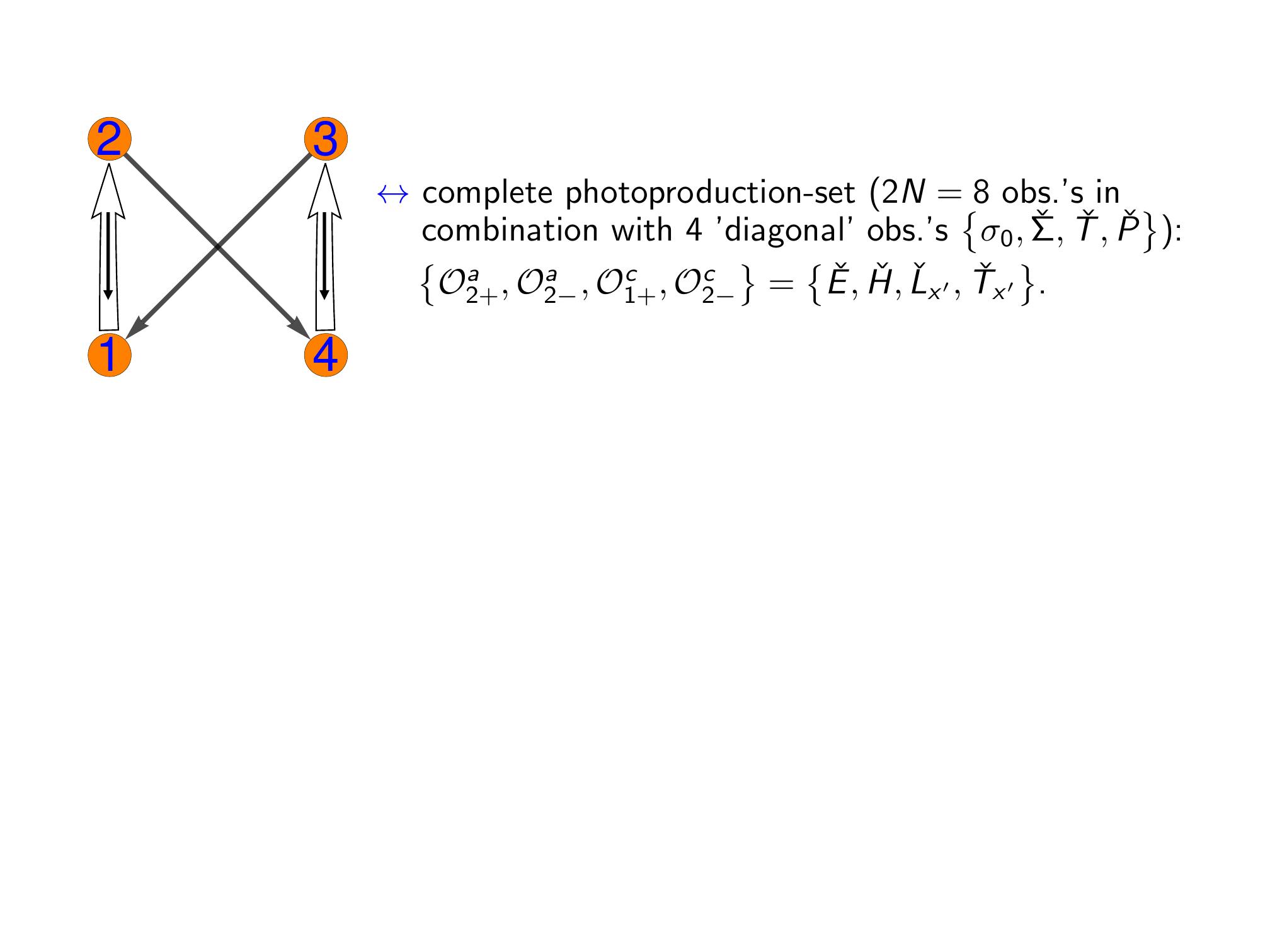
In order to reduce the mismatch between the results of Moravcsik’s theorem and the absolutely minimal length of $2N$ observables in a complete set (cf. sec 5), new graphs have been proposed in reference [30], which contain additional directional information. The new completeness criterion for these graphs makes heavy use of the repeating mathematical structure of non-diagonal ’shape-classes of $4$’ (cf. Table 1). One example for a ’directional’ graph for photoproduction ($N=4$), as well as a corresponding complete set, is shown in Figure 6. The new graphs contain [30]:

• -

  Single-lined arrows, which have the same meaning as in Moravcsik’s theorem (sec. 4).

• -

  Double-lined arrows denoting ’crossed’ selections of observable-pairs, i.e. $\mathcal{O}^{n}_{1\pm}$ $\oplus$ $\mathcal{O}^{n}_{2\pm}$ (e.g.: $\left(\mathcal{O}^{n}_{1+},\mathcal{O}^{n}_{2+}\right)$).

• -

  An ’outer’ direction which is in direct correspondence to a directional convention for indices appearing in the consistency relation. For the graph in Figure 6, the consistency relation reads: $\phi_{12}+\phi_{24}+\phi_{43}+\phi_{31}=0$.

• -

  The direction of smaller ’inner’ arrows inside of double-lined arrows, which specifies the sign of ’$\zeta$-angles’ appearing in the formulas for discrete phase-ambiguities (see [30]). The $\zeta$-angles are important for removing dependencies among consistency relations.

• $\Rightarrow$

  The graph in Figure 6, for example, is complete because the ’inner’ arrows both point opposite to the bigger double-lined arrows (cf. explanations in ref. [30]).

Using these new graphs, $60$ known complete sets of minimal length $2N$ have been re-derived for photoproduction and $1216$ new such sets have been found for electroproduction (see ref. [30]). Reactions with $N>6$ amplitudes likely require new and more involved algebraic derivations [30].

The graphical methods discussed up to this point show their real utility once applied to problems with larger numbers of amplitudes, for instance $N>6$. The connectedness of the graphs automatically removes continuous ambiguities and it ensures the possibility to write down a consistency relation, two tasks which can become rather awkward when done ’by hand’ for problems with higher $N$.

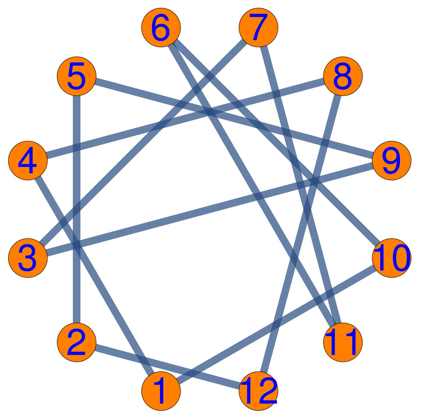
For two-meson photoproduction ($N=8$) [34], the selection of complete sets from the full set of $N^{2}=64$ observables proceeds via $\frac{(N-1)!}{2}=2520$ connected start-topologies. One example for a fully complete graph according to Moravcsik (sec. 4) is shown in Figure 7, on the left. In reference [35], it was found that the Moravcsik-complete sets for this problem contain at least $24$ observables. Numerical as well as algebraic methods were than applied to reduce these sets to the minimal length of $2N=16$. For more details on applications to two-meson photoproduction, see the contribution [36] to this conference.

For vector-meson photoproduction ($N=12$) [37], one examplary connected start-topology is shown in Figure 7, on the right. The graphical solution to this problem can be automated on a computer, even though the number of $\frac{(N-1)!}{2}=19958400$ connected start-topologies may look a bit intimidating. Vector-meson photoproduction is a possible future option for applications of the methods presented here.

Graphical methods for the determination of complete experiments have been discussed. These methods have reproduced already known results for reactions with relatively few spin amplitudes, e.g. single-meson photoproduction ($N=4$ amplitudes). The real power of such graphical methods lies in their capability to derive complete sets for more complicated reactions, i.e. with higher numbers of $N>6$ spin amplitudes, where these methods should be applied in order to help plan future measurements in baryon spectroscopy.

References

- . E. Klempt and J. M. Richard, Rev. Mod. Phys. 82, 1095 (2010) doi:10.1103/RevModPhys.82.1095 [arXiv:0901.2055 [hep-ph]].
- . V. Crede and W. Roberts, Rept. Prog. Phys. 76, 076301 (2013) doi:10.1088/0034-4885/76/7/076301 [arXiv:1302.7299 [nucl-ex]].
- . D. G. Ireland, E. Pasyuk and I. Strakovsky, Prog. Part. Nucl. Phys. 111, 103752 (2020) doi:10.1016/j.ppnp.2019.103752 [arXiv:1906.04228 [nucl-ex]].
- . A. Thiel et al., Phys. Rev. Lett. 109, 102001 (2012) doi:10.1103/PhysRevLett.109.102001, 10.1103/PhysRevLett.110.169102, 10.1103/PhysRevLett.110.169101 [arXiv:1207.2686 [nucl-ex]].
- . M. Gottschall et al. [CBELSA/TAPS], Phys. Rev. Lett. 112, no.1, 012003 (2014) doi:10.1103/PhysRevLett.112.012003 [arXiv:1312.2187 [nucl-ex]].
- . J. Hartmann et al., Phys. Rev. Lett. 113, 062001 (2014) doi:10.1103/PhysRevLett.113.062001 [arXiv:1407.2163 [nucl-ex]].
- . F. Afzal et al. [CBELSA/TAPS], Phys. Rev. Lett. 125, no.15, 152002 (2020) doi:10.1103/PhysRevLett.125.152002 [arXiv:2009.06248 [nucl-ex]].
- . M. Dugger et al. [CLAS], Phys. Rev. C 88, no.6, 065203 (2013) doi:10.1103/PhysRevC.88.065203 [arXiv:1308.4028 [nucl-ex]].
- . P. Collins et al. [CLAS], Phys. Lett. B 771, 213-221 (2017) doi:10.1016/j.physletb.2017.05.045 [arXiv:1703.00433 [nucl-ex]].
- . I. Senderovich et al. [CLAS], Phys. Lett. B 755, 64-69 (2016) doi:10.1016/j.physletb.2016.01.044 [arXiv:1507.00325 [nucl-ex]].
- . S. Strauch et al. [CLAS], Phys. Lett. B 750, 53-58 (2015) doi:10.1016/j.physletb.2015.08.053 [arXiv:1503.05163 [nucl-ex]].
- . V. D. Burkert, EPJ Web Conf. 241, 01004 (2020) doi:10.1051/epjconf/202024101004 [arXiv:1912.11400 [nucl-ex]].
- . V. Burkert et al., Nucl. Instrum. Meth. A 959, 163419 (2020) doi:10.1016/j.nima.2020.163419
- . D. Hornidge et al. [A2 and CB-TAPS], Phys. Rev. Lett. 111, no.6, 062004 (2013) doi:10.1103/PhysRevLett.111.062004 [arXiv:1211.5495 [nucl-ex]].
- . P. Adlarson et al. [A2], Phys. Rev. C 92, no.2, 024617 (2015) doi:10.1103/PhysRevC.92.024617 [arXiv:1506.08849 [hep-ex]].
- . S. Gardner et al. [MAINZ-A2], Eur. Phys. J. A 52, no.11, 333 (2016) doi:10.1140/epja/i2016-16333-5 [arXiv:1606.07930 [nucl-ex]].
- . J. Annand et al. [A2 and MAMI], Phys. Rev. C 93, no.5, 055209 (2016) doi:10.1103/PhysRevC.93.055209
- . V. L. Kashevarov et al. [A2 Collaboration], Phys. Rev. Lett. 118, no. 21, 212001 (2017).
- . W. Briscoe et al. [A2], Phys. Rev. C 100, no.6, 065205 (2019) doi:10.1103/PhysRevC.100.065205 [arXiv:1908.02730 [nucl-ex]].
- . H. Kohri et al. [LEPS], Phys. Rev. C 97, no.1, 015205 (2018) doi:10.1103/PhysRevC.97.015205 [arXiv:1708.09574 [nucl-ex]].
- . H. Kohri [LEPS], EPJ Web Conf. 241, 01010 (2020) doi:10.1051/epjconf/202024101010
- . H. Al Ghoul et al. [GlueX], Phys. Rev. C 95, no.4, 042201 (2017) doi:10.1103/PhysRevC.95.042201 [arXiv:1701.08123 [nucl-ex]].
- . S. Adhikari et al. [GlueX], Phys. Rev. C 100, no.5, 052201 (2019) doi:10.1103/PhysRevC.100.052201 [arXiv:1908.05563 [nucl-ex]].
- . S. Adhikari et al. [GlueX], Nucl. Instrum. Meth. A 987, 164807 (2021) doi:10.1016/j.nima.2020.164807 [arXiv:2005.14272 [physics.ins-det]].
- . I. S. Barker, A. Donnachie and J. K. Storrow, Nucl. Phys. B 95, 347 (1975). doi:10.1016/0550-3213(75)90049-8
- . G. Keaton and R. Workman, Phys. Rev. C 53, 1434-1436 (1996) doi:10.1103/PhysRevC.53.1434 [arXiv:nucl-th/9511040 [nucl-th]].
- . W. T. Chiang and F. Tabakin, Phys. Rev. C 55, 2054 (1997) doi:10.1103/PhysRevC.55.2054 [nucl-th/9611053].
- . K. Nakayama, Phys. Rev. C 100, no. 3, 035208 (2019) doi:10.1103/PhysRevC.100.035208 [arXiv:1809.00335 [nucl-th]].
- . Y. Wunderlich, P. Kroenert, F. Afzal and A. Thiel, Phys. Rev. C 102, no.3, 034605 (2020) doi:10.1103/PhysRevC.102.034605 [arXiv:2004.14483 [nucl-th]].
- . Y. Wunderlich, Phys. Rev. C 104, no.4, 045203 (2021) doi:10.1103/PhysRevC.104.045203 [arXiv:2106.00486 [nucl-th]].
- . G. Keaton and R. Workman, Phys. Rev. C 54, 1437-1440 (1996) doi:10.1103/PhysRevC.54.1437 [arXiv:nucl-th/9606052 [nucl-th]].
- . M. J. Moravcsik, J. Math. Phys. 26, 211 (1985). doi:10.1063/1.526787
- . L. Tiator, R. L. Workman, Y. Wunderlich and H. Haberzettl, Phys. Rev. C 96, no. 2, 025210 (2017) doi:10.1103/PhysRevC.96.025210 [arXiv:1702.08375 [nucl-th]].
- . W. Roberts and T. Oed, Phys. Rev. C 71, 055201 (2005) doi:10.1103/PhysRevC.71.055201 [nucl-th/0410012].
- . P. Kroenert, Y. Wunderlich, F. Afzal and A. Thiel, Phys. Rev. C 103, no.1, 014607 (2021) doi:10.1103/PhysRevC.103.014607 [arXiv:2009.04356 [nucl-th]].
- . P. Kroenert, “Minimal complete sets for two pseudoscalar meson photoproduction,” contribution to HADRON 2021 (2021).
- . M. Pichowsky, C. Savkli and F. Tabakin, Phys. Rev. C 53, 593 (1996) doi:10.1103/PhysRevC.53.593 [nucl-th/9509022].