A Novel Compartmental Approach to Modeling COVID-19 Disease Dynamics and Analyzing the Effect of Common Preventative Measures
Abstract
As of December 2020, the COVID-19 pandemic has infected over 75 million people, making it the deadliest pandemic in modern history. This study develops a novel compartmental epidemiological model specific to the SARS-CoV-2 virus and analyzes the effect of common preventative measures such as testing, quarantine, social distancing, and vaccination. By accounting for the most prevalent interventions that have been enacted to minimize the spread of the virus, the model establishes a paramount foundation for future mathematical modeling of COVID-19 and other modern pandemics. Specifically, the model expands on the classic SIR model and introduces separate compartments for individuals who are in the incubation period, asymptomatic, tested-positive, quarantined, vaccinated, or deceased. It also accounts for variable infection, testing, and death rates. I first analyze the outbreak in Santa Clara County, California, and later generalize the findings. The results show that—although all preventative measures reduce the spread of COVID-19—quarantine and social distancing mandates reduce the infection rate and subsequently are the most effective policies, followed by vaccine distribution and, finally, public testing. Thus, governments should concentrate resources on enforcing quarantine and social distancing policies. In addition, I find mathematical proof that the relatively high asymptomatic rate and long incubation period are driving factors of COVID-19’s rapid spread.
1 Introduction
1.1 The COVID-19 Pandemic
The emergence of a new strain of coronavirus named SARS-CoV-2 in Wuhan, China in December of 2019 has led to the global COVID-19 pandemic that has affected all worldwide operations. The respiratory infection—which causes symptoms such as a fever, cough, and difficulty breathing—has been confirmed to have infected over 75 million individuals and caused nearly 2.0 million deaths globally as of December 2020, though the actual numbers are significantly higher due to the presence of undetected infections [1, 2]. The casualty toll of the pandemic is far greater than any other disease outbreak in recent history and continues to grow worse [3].
Unsurprisingly, many researchers have attempted to model COVID-19 [4]. Compartmental epidemiological models are typically the most common, but many other methodologies are used [5]. For instance, [6] use a Bayesian model, [7] use ridge regression, and [8] use machine learning. Of these studies, some derive models specific to SARS-CoV-2 and the COVID-19 pandemic: [9] create a compartmental model that accounts for hospitalizations and super-spreaders, while [10] develop a compartmental model that considers a variable infection rate and critical vs. noncritical infections. Such models attempt to forecast the pandemic more accurately by considering nuances of the SARS-CoV-2 virus that make it particularly infectious.
In attempt to control the spread of the virus, governments around the world have imposed preventative measures such as quarantines, shelter-in-place lockdowns, mask enforcement, and widespread testing [11]. Despite such attempts, cases around the world continue to rise, and the economic and social consequences of the pandemic grow worse. Governments also have limited resources, and citizens have a finite tolerance for preventative measures [12, 13]. Still, such measures have been found to significantly reduce spread [14, 15, 16]. Thus, in addition to forecasting the virus’s spread, identifying and analyzing common preventative measures are key to ending the pandemic.
1.2 Research Focus
To my knowledge, none of the models specific to COVID-19 analyze the impact of individual preventative measures. In addition, none conduct quantitative investigations that study which measures are more effective than others. Because there is a finite amount of regulation that can be used enforced, it is important to study which measures should be prioritized. Therefore, this paper consists of three main goals:
- 1.
Develop an accurate model specific to the COVID-19 pandemic that accounts for nuances of SARS-CoV-2 and common preventative measures implemented during the pandemic
- 2.
Perform a case study with the model in one specific region to study its validity
- 3.
Analyze the effect of common preventative measures and determine which are most effective
2 Developing a Model
2.1 Methodology and Considerations
Mathematical modeling can be classified as either data-driven—which allows one to derive equations directly from empirical data—or mechanistic, which uses the data to derive equations that can model a phenomenon. While data-driven models can make accurate predictions, they often fail to provide meaningful physical interpretations of the occurrence and only produce results. In other words, they can predict what will happen without explaining why. In this study, I make some assumptions that allow us to adopt mechanistic models for the research and derive a system of equations that can capture key dynamics of the outbreak such as the number of infected individuals for any amount of time in the future. The equations account for social distancing precautions, asymptomatic cases, testing, quarantine, a potential vaccine, and death. Throughout the study, social distancing will refer to any measure taken by all individuals to reduce the spread of the pandemic, which includes practices such as limiting non-essential travel or wearing masks.

2.2 Developing the Model
The most reasonable methodology is the utilization of a compartmental epidemiological model, a method first developed in 1927 as the result of research by mathematicians and epidemiologists Anderson Gray McKendrick and William Ogilvy Kermack [17]. Compartmental models in epidemiology divide a given population into various categories and characterize the dynamics of each population using differential equations. For instance, the works of Kermack and McKendrick began with the simple SIR model, which creates three compartments: susceptible, infected, and recovered.


However, the model has since been adapted and expanded upon, leading to the creation of new compartmental models, such as the SEIR model—which considers incubation periods—and the MSIR model which accounts for maternally-derived immunity [19, 20]. Some compartmental models also account for variable contact rates, which are more realistic as they reflect changes in the infection rate as an outbreak progresses [21]. For this study, the following information should be considered:
- 1.
- 2.
- 3.
- 4.
There are a significant number of deaths resulting from COVID-19, pointing to the need for a specific category for deceased individuals [29].
- •
However, the death rate is not fixed. As hospitals and other healthcare services adapt to the pandemic, fewer infections are fatal. This suggests a variable death rate.
- •
- 5.
There should be a compartment for vaccinated individuals who, like the recovered category, have immunity against the disease. The model should also consider the possibility that the vaccine is partially ineffective.
- 6.
I must account for variations in social distancing that would phenomenologically affect the infection rate of the disease, suggesting a variable infection rate.
- 7.
Widespread testing can reduce the spread of COVID-19 by identifying asymptomatic individuals [30]. However, the entire population cannot be tested. Thus, I classify asymptomatic individuals as having been tested or not.
- •
However, as the availability of COVID-19 tests increases over time, more asymptomatic cases are identified, suggesting the need for a variable testing rate.
- •
2.3 Outline of the Model
Thus, the classifications that the model requires are as follows: susceptible (), incubation (), asymptomatic (), asymptomatic-and-quarantined (due to a positive test, ), symptomatic-and-quarantined (), vaccinated (), recovered (), and dead (). Also, the infection, testing, and death rates are variable, producing a SIAPQVRD model with variable rates.

Susceptible individuals, who are the vast majority of the population, can become infected or vaccinated. If vaccinated successfully, an individual moves directly into the vaccinated category. If infected, an individual first enters an incubation period. Those who eventually exhibit symptoms move into the symptomatic (quarantined) category, while asymptomatic cases move to the asymptomatic compartment.
Asymptomatic individuals ( or ) who are tested for COVID-19 move into the tested-positive category. The model separates symptomatic (quarantined) individuals and asymptomatic individuals who have tested positive (also quarantined) because only symptomatic individuals can die of COVID-19.
If symptomatic, individuals can either move into the recovered category or the dead category. All asymptomatic cases recover.
2.4 Key Assumptions and Simplifications
The following assumptions and simplifications are made and referenced throughout the report. Justifications, explanations, and implications of the assumptions are discussed in the conclusion.
- 1.
The law of mass action is maintained. That is, the total rate of encounters (collision frequency) between individuals of two different categories is proportional to the product of their concentrations.
- 2.
Natural birth and death rates are negligible relative to the total population.
- 3.
All individuals follow social distancing measures, and all individuals with a confirmed infection quarantine.
- 4.
Only the vaccination of susceptible individuals is tracked.
- 5.
Only one dose of the vaccine is required, and, if successful, provides immunity immediately.
- 6.
Only the testing of susceptible and asymptomatic individuals is tracked.
- 7.
Testing is perfect (no false positives or negatives) and completely random.
3 Deriving the Model
As shown in Figure 2 and Figure 3, in compartmental epidemiological modeling, events such as infection or vaccination cause individuals to move from one category into another. In this section, I determine the mathematical basis of these movements.
3.1 Susceptible
All individuals, except patient zero, begin susceptible. Traditionally, individuals can only move out of the susceptible population through infection; in the SIAPQVRD model, they can be vaccinated as well. Here, I will discuss the former, and vaccination will be incorporated in Section 3.6.
The rate at which people become infected is controlled by the number of susceptible people, the number of infected people, and the infection rate. I incorporate a variable infection rate with the form:
Each represents a different stage of the infection rate. My model also considers unknown cases, which have different infection rates. Thus, I divide into two categories: and , which refer to the infection rate for known and unknown cases respectively. Both will be divided as by constants, and , to scale their values:
Since the SIAPQVRD has four categories of infected individuals that can all cause secondary infections, I must include all of them in the equation for . Thus,
| (1) |
3.2 Incubation
All infected individuals first enter an incubation period. To exit , one must either exit the incubation period or be tested for COVID-19. Thus,
Let be the incubation rate, or the fraction of the population that exits the incubation period daily. Let be the variable testing rate: a fraction of the tested population is tested daily. Let be the testing parameter. I incorporate a variable testing rate:
The testing parameter scales the testing rate by a constant, which allows us to tune the testing rate during my analysis. For instance, doubling and simulating an outbreak under otherwise equal conditions explores the effect of doubling the testing rate. Thus,
| (2) |
3.3 Asymptomatic
Individuals enter the asymptomatic category from the incubation category and exit to the recovered category or the tested-positive category. Thus,
Let be the rate of asymptomatic infections, or the fraction of total cases that are asymptomatic. Let be the recovery rate for asymptomatic infections: a fraction of the asymptomatic category recovers each day. Thus,
| (3) |
3.4 Tested-Positive
People move into from or by being tested. The only way to exit is by recovering. Thus:
Anyone in is asymptomatic and therefore has a recovery rate . Thus,
| (4) |
3.5 Quarantine
People enter by developing a symptomatic infection and consequently quarantining. People exit by recovering or dying. Thus,
Any infection that is not asymptomatic is symptomatic, so the rate of symptomatic infections is . Let be the recovery rate for symptomatic infections and let be the variable death rate (a fraction of dies daily).
3.5.1 Death Rate
The death rate changes over time as hospitals and other services adapt to the pandemic. Thus, I include a variable death rate:
Thus,
| (5) |
3.6 Vaccinated
People enter from by receiving a successful vaccination, and people cannot exit . Let be the vaccination rate (a fraction of is vaccinated daily). Let be the success rate of the vaccination (a fraction of vaccines are successful in preventing COVID-19). Unsuccessful vaccines have no effect. Combined, a product and of are vaccinated daily. Therefore,
| (6) |
From equation (1), we now have:
| (7) |
3.7 Recovered
People enter by recovering from an infection, either symptomatic or asymptomatic, and cannot exit:
| (8) |
3.8 Dead
People enter by dying and cannot exit:
| (9) |
3.9 Complete System
The complete system is:
| (10) | ||||

The total population should not change. That is,
| (11) |
This can be confirmed by taking the sum of the equations in (10).
Like most compartmental epidemiological models, each compartment will represent a fraction of the total population, rather than the true number of individuals in the category. Thus, .
3.10 Summary of State Variables and Parameters
the fraction of the population that is susceptible.
the fraction of the population that is in the incubation period.
the fraction of the population that is asymptomatic and has not been tested and is therefore not quarantined.
the fraction of the population that is asymptomatic and has been tested and quarantined.
the fraction of the population that is quarantined because they are exhibiting symptoms.
the fraction of the population that is vaccinated.
the fraction of the population that has recovered.
the fraction of the population that has died of infection.
= the variable infection rate for asymptomatic individuals that accounts for preventative measures that are taken by the entire population (e.g., social distancing or mask-wearing). controls the effectiveness of these measures. Each asymptomatic person infects, on average, other people per day.
the infection rate for individuals who are quarantined (symptomatic or asymptomatic and tested-positive), who therefore have a lower infection rate [31]. governs how strict the quarantine is. Each symptomatic or tested-positive person infects, on average, other people per day.
the recovery rate for asymptomatic individuals. A fraction of the asymptomatic population recovers every day. is the average recovery duration for asymptomatic infections.
the recovery rate for symptomatic individuals. A fraction of the symptomatic population recovers every day. is the average recovery duration for symptomatic infections.
= the rate at which people with symptomatic infections begin to exhibit symptoms. the average incubation period.
the variable testing rate. A fraction of the population is tested daily.
the asymptomatic rate. A fraction of cases are asymptomatic.
the rate of vaccination, which reflects the availability of the vaccine. A fraction of the susceptible population is vaccinated every day.
the success rate of the vaccine. A fraction of vaccinations prevent infection.
= the variable death rate. A fraction of the symptomatic population dies daily.
4 Determining Parameter Values
To determine specific parameter values, I apply the model to Santa Clara County, CA, which has a population of 1,928,000 and 75,000 cumulative cases at the time of writing [32, 33].
4.1 General Parameters
Some parameters are inherent to the SARS-CoV-2 virus:
| Parameter | Meaning | Value |
| Asymptomatic rate | 0.31 | |
| Incubation rate | ||
| Asymptomatic recovery rate | ||
| Symptomatic recovery rate | ||
| Vaccine success rate | 0.90 |
The remaining parameters are calculated specifically for Santa Clara County. In the following calculations, data collection began on March 2, 2020 () and ended on December 7, 2020 ().
4.2 Infection Rate
To determine , I use publicly released information on COVID-19 in Santa Clara County and calculate the infection rate by dividing the number of new cases per day by the total number of known, active cases. Then, I take a seven-day moving average of the values, yielding:

4.2.1 Approximation of Current Cases
Because there is no way to determine the true number of active cases at any given time, I make an approximation. Letting represent the number of known active cases at time :
| (12) |
4.2.2 Accounting for Asymptomatic Infections
In calculating , I assume that the number of known cases reported by the county is equal to the total number of infections, as it is impossible to determine the true number of asymptomatic cases. Due to this approximation, this is not a true representation of the infection rate as it fails to account for asymptomatic cases. However, the function still provides a mechanistic view of the infection rate over time: if this approximated increases, then the true infection rate also is increasing. I assume that the difference between the calculated and the true infection is the absence of a scalar multiple, which is taken into consideration by the parameters and . I will estimate the specific values of and once the remaining parameters are determined.
4.3 Testing Rate
I perform a similar analysis with the testing rate. I take the number of raw tests daily and divide it by the total population to determine .

4.4 Death Rate
The death rate is determined in the same way. I take the number of daily deaths and divide them by the estimated number of active cases to obtain the death rate on that day.

This plot yields:
4.5 Determining and
Unlike other parameters, there is no official value for or : I must determine it through experimentation. The role of and is twofold: first, to consider that people who know they are infected will quarantine themselves, while others will only follow common measures such as social distancing; and second, to account for the simplification made in determining that disregards asymptomatic cases. If these purposes are unaccounted for, then the infection rate used will be too large, as the the infection rate is calculated by dividing the daily number of new cases by the product of and the total cases. If I assume that all cases are reported, then I ignore asymptomatic cases, and the total cases will be lower than they should be.
Since was calculated by disregarding asymptomatic cases, it reflects regular social behavior of people who do not believe that they are infected, regardless of whether they actually are. Thus, by default, I set . This approximation does not stand for individuals who know they are infected, as they would quarantine, thereby reducing their infection rate. To determine the exact value of , I experiment with different values and simulate hypothetical outbreaks until I most closely resemble the actual outbreak in Santa Clara County, which occurs at .
4.6 Applying the Model to the COVID Outbreak in Santa Clara County
I now have a complete model with parameter values and functions. To test the validity of the model, I assumed initial conditions based on the COVID-19 data for Santa Clara County.
| Population | Initial Value |
|---|---|
| 0.991141 | |
| 0.000001 | |
| 0.000001 | |
| 0.00000241182 |
| Population | Initial Value |
|---|---|
| 0.00000241182 | |
| 0 | |
| 0.00884728 | |
| 0.000001556 |
Numerically solving the system using a Fourth-Order Runge-Kutta approximation in Mathematica returns:


Figure 8a shows that there is a significant population of asymptomatic cases (, shown in magenta) at all times, demonstrating that the number of cases is drastically underreported. The value of , shown in green, is very small, which indicates that testing does not identify a significant number of cases. This also explains why my assumption in calculating the death rate is almost insignificant: almost all of the reported cases are symptomatic and therefore could cause death. However, the effect of testing may be understated due to the assumption of random testing. In reality, testing is not random; those who believe they may have been exposed to the virus are more likely to be tested.
5 Analyzing Preventative Measures
The most significant purpose of this study is to analyze the effect that preventative measures have on containing the pandemic and determine which measures are most significant. Because the model includes parameters that dictate different aspects of the virus or different preventative measures, parameters can be tuned to explore possible outbreaks under different conditions. To accomplish this, the independent variable must be a parameter instead of time; and, to isolate the effect of each parameter, only one parameter will be tuned at once. The dependent variable will be the number of cases and deaths by .
5.1 Social Distancing and Quarantine
Social distancing and quarantine are two of the most common preventative measures [39]. In the model, they are represented by and respectively and scale the infection rate. Thus, tuning and illustrates the significance of the infection rate:


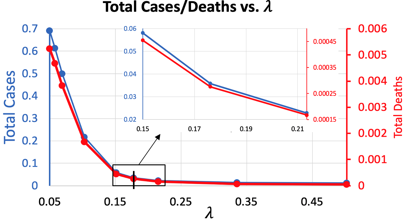
Figure 9 shows that and have a very significant effect on the dynamics of the outbreak. The relationship is exponential: the infection rate has a significantly larger effect at larger values (smaller values of and ). At smaller infection rates, variations in and have little to no effect, as demonstrated up close for in 9a.
5.2 Testing
Testing has been adopted and strongly encouraged strongly by governments to identify asymptomatic cases and track the outbreak [40]. More testing slows the spread of the virus because more asymptomatic cases are identified and more quarantining occurs. With the addition of , I can tune the testing rate .

5.3 Vaccination
A vaccine with 90% effectiveness () against SARS-CoV-2 has recently been released by industrial pharmaceutical company Pfizer [38]. It is important to investigate the potential effect that this vaccine will have in controlling the outbreak, which will be done by tuning , the availability of the vaccine.


5.4 Phase Times
Due to the incorporation of a variable infection rate that takes the form of a piecewise function, I can explore the effect that different phase times of , or different social behavior patterns, would have. For instance, by extending , a phase of exponential decline in the infection rate, I can examine the potential outbreak that could have occurred if initial social behavior was maintained.


5.5 Summary and Key Findings
The study of common preventative measures is the most novel and significant aspect of the research. The following tables summarize the primary findings:
| Parameter | 10% Increase () | 25% Increase () | 50% Increase () |
|---|---|---|---|
| 40.54% | 64.86% | 72.97% | |
| 29.73% | 52.51% | 60.89% | |
| 11.23% | 26.34% | 45.86% | |
| 0.56% | 1.39% | 2.78% |
As discussed in the individual sections and shown in Table 1, the preventative measures studied have varying levels of significance. Reducing the infection rate, which is done mathematically by increasing or , is the single most important method of reducing spread. Translating these findings to the real world, this means that governments and individuals alike must concentrate on social distancing, wearing masks, reducing non-essential travel, quarantining appropriately, etc. Attempting to substitute such measures with widespread testing—which has an almost trivial impact in comparison—would fail to control the spread of the outbreak. Meanwhile, the ongoing distribution of the vaccine must be continued, as public vaccination—like reducing the infection rate—significantly reduces the spread of the virus.
6 Other Parameters
Although other strains of coronaviruses have emerged in the past, COVID-19 has been particularly contagious [41, 42]. Some researchers have attributed this to its long incubation period and high rate of asymptomatic cases relative to other diseases [43]. By tuning the incubation rate and the asymptomatic rate , I can investigate the significance of these two parameters:

As expected, the total number of cases increases alongside , as a higher rate of asymptomatic infection would lead to more unknown cases, whose infection rates are given by ; is greater than , the infection rate for known, quarantined infections. However, the relationship between total deaths and is more interesting, as it contains both upwards and downwards-sloping segments. Total deaths increase alongside until , making the deadliest asymptomatic rate. This correlation can be explained easily: more asymptomatic infections increase the total number of cases, while also creating fewer deadly cases (since only symptomatic infections can cause death).
6.1 Death Rate
Finally, I can investigate the effect of changing the death rate. Notice that there is no parameter incorporated into the model that scales the death rate because I do not wish to tune the entire death rate, but instead only the first two stages, where the death rate was changing rapidly. In stages 3 and 4, the death rate is nearly constant, which I assume to be the equilibrium stage of the death rate where healthcare services are properly equipped to handle the outbreak. Only in the first two stages were these services still adapting to the pandemic, resulting in large fluctuations in the rate of fatal infections. It is these fluctuations that I wish to model. Therefore, in this section, I manually scale the first two stages of the death rate.
The death rate has a marginal effect on the number of cases since such a small portion of infections are deadly. Thus, it seems only necessary to study the effect of changing the death rate on the actual number of deaths.

Although both situations significantly lower the death rate, such changes do not produce equally significant effects. This is because, during the first two stages, the outbreak was not as widespread, and—although the death rate was higher—there were few cases and therefore few total fatalities. Although the death rate was lower during the third and fourth stages, the brunt of the infections occurred during these phases, thereby producing the majority of the deaths.
7 Conclusion
As the COVID-19 pandemic continues to surge, lives are lost and social and economic repercussions grow worse. Forecasting and mitigating the spread of the pandemic are more important than ever. In this study, I develop a compartmental model specific to the COVID-19 pandemic that accounts for common preventative measures that have been imposed, apply the model to a real-world case study, and use the model to analyze the effect of common preventative measures.
To accomplish this, I derive a novel compartmental epidemiological model that expands on the classic SIR model and accounts for the incubation period, asymptomatic infections, testing, quarantine, vaccination, and death. In addition, I consider the real-world dynamics that lead to variable infection, testing, and death rates. Then, I apply this model to Santa Clara County, California, and, by tuning the model’s parameters, I determine the extent to which common preventative measures contain the spread of the virus. Additionally, I study two of the characteristics of SARS-CoV-2 that make COVID-19 particularly contagious.
7.1 Key Findings
I develop a novel SIAPQVRD model that includes eight categories: susceptible (), incubation (), asymptomatic (), asymptomatic and quarantined due to a positive test (), symptomatic and quarantined(), recovered (), vaccinated (), and dead (). In addition, I include variable infection, testing, and death rates.
To apply the model to Santa Clara County, I take publicly-released COVID-19 data and derive functions for the infection, testing, and death rates. I find that the infection rate can be classified into five distinct phases, reflect changes social interactions over time. The testing rate rises consistently over time and can also be divided into five stages that each represent different rates of growth. The death rate can be divided into four stages, which reflects the adaptation of healthcare services. The remaining parameters were determined using external research on COVID-19, except , which was found experimentally.
I first compare the model’s predictions with actual data by inputting initial conditions and find that it is reasonably accurate, albeit with minor discrepancies. Then, to investigate the effect of preventative measures, I tune parameters in the model individually while holding the others constant, making the tuned parameter the independent variable and the total number of cases and deaths by the time of writing the dependent variable. I find that controlling the infection rate through parameters and has the most significant impact on containing the virus. A vaccination also has a significant effect on reducing viral transmission, with a more available vaccine and a greater duration of availability producing a substantially stronger effect. Testing, however, barely has a noticeable impact, even at very high levels. By experimenting with different phase times for the infection rate, I also find that reducing social behavior to prevent the infection rate from rising is critical to minimize transmission. Indeed, reverting to initial social interaction levels could end the pandemic shortly.
I also investigate the effect of tuning the incubation period and rate of asymptomatic infections, and I find that both have a significant effect. Indeed, the long incubation period and high rate of asymptomatic cases relative to other diseases appear to be driving causes of COVID-19’s rapid spread. Decreases in the incubation period exponentially decrease total cases and deaths, while increases in the asymptomatic rate also exponentially increase total cases. The asymptomatic rate increases the number of deaths for and decreases the number of deaths for
7.2 Implications and Applications of the Findings
7.2.1 General SIAPQVRD Model
The model is a novel development in compartmental epidemiological modeling. Although it was designed specifically for COVID-19, many infectious diseases also involve a significant incubation period and cause asymptomatic infections, such as the H1N1 influenza virus or MERS-CoV [44, 45]. In addition, any modern pandemic will also involve the implementation of the preventative measures studied—social distancing, quarantine, widespread testing, and vaccination. Thus, the model is not exclusive to COVID-19 and lays a paramount foundation for the mathematical modeling of forecasting future pandemics.
7.2.2 Case Study of Santa Clara County, CA
First, the observation that shows that quarantined individuals still have a reasonably high infection rate, creating only approximately 1.75 fewer secondary infections per day than unknown, asymptomatic infections. This proves that individuals who know they are infected and contagious still maintain relatively high levels of social interactions. In an ideal situation with a perfect quarantine, . I find that increasing to a sufficiently high number could reduce total cases and deaths by over three times. The implication is twofold: first, that individuals who are symptomatic or have been tested positive for COVID-19 must quarantine themselves more effectively; second, that governments must enforce stricter regulations that mandate the quarantine of anyone with a known infection.
Second, I discover that the death rate rises and then falls rapidly at the beginning of the outbreak. Afterward, it remains nearly constant. This indicates that hospitals and other public services are initially unprepared to handle surges in cases. As such facilities adapt, despite increases in the number of cases, they treat patients more effectively, thereby reducing the death rate. I find that if hospitals were better-equipped initially and the death rate during the spike was reduced twofold, total deaths could be reduced by . In an ideal situation where such services were fully prepared from the beginning (i.e. the death rate was at the equilibrium value from the start), total deaths could be reduced by . Although such reductions would not be particularly significant in Santa Clara County, where there have been few COVID-19 deaths altogether, they could have much more meaningful effects in areas hit harder by the pandemic.
7.2.3 Study of Preventative Measures
My study of key preventative measures has the most real-world implications. First, I notice that tuning and , which scale the infection rate, has a dramatic effect on the outbreak, with minor increases in either parameter resulting in very significant declines in the number of cases and deaths. Therefore, governments’ first priorities should be to minimize the infection rate. Although I reference as the social distancing parameter throughout the study, it more generally refers to the regular social patterns of all individuals; therefore, any preventive measure that is adopted by all individuals such as mask-wearing or minimizing non-essential travel would increase . To increase , a stronger quarantine for those who know they are infected should be enforced.
I also find that if social behavior followed the same pattern as it did during the first stage of the infection rate, the pandemic in Santa Clara County would have ended in just 75 days. The upcoming spike can also be avoided by reverting to previous levels of social patterns, where the infection rate declined linearly, albeit slowly. Therefore, I find that the number one method to reduce viral transmission is to ensure that the infection rate does not rise; even minor decreases in the infection will, over time, force an end to the outbreak. In the scope of the model, this makes sense: if the infection rate increases linearly, then the rate at which people spread the disease increases linearly, causing the number of infections to rise exponentially.
Unlike the infection rate, testing has a much smaller effect on controlling the outbreak, with a twofold increase in the testing rate reducing total cases and deaths by . The implication is first that testing will never reach adequately significant levels to have a meaningful reduction in transmission; and, second, that even with high testing rates, testing is insignificant because those who receive a positive test do not quarantine themselves adequately. Thus, governments should consider channeling resources away from testing towards increasing other preventative measures that could have a more significant impact on reducing the outbreak. Meanwhile, governments should impose regulations or spread information that results in stronger quarantines; if quarantines are adequately effective, then testing can have a stronger preventative impact, as those with an asymptomatic infection who receive a test will spread the virus at greatly reduced rate.
The distribution of the vaccine will have a significant impact on reducing the spread of the virus. Increasing the availability of the vaccine is particularly important, especially at lower availabilities. Therefore, alongside reducing the infection rate, governments should prioritize distributing the vaccine as fast as possible.
Interestingly, the death rate has a small effect on reducing the death count. Even if public services such as hospitals were properly equipped from the beginning, total deaths would have been reduced by only 20%. This is because most infections occurred once the death rate had stabilized. Therefore, I can conclude that although ill-prepared initially, such services reacted in adequate time to ensure that the death rate was reduced for the majority of the outbreak. Therefore, although better-equipped hospitals can save a moderate number of lives, in future pandemics, governments can direct more attention to reducing the number of infections, which is the true driver of fatalities.
I also find that longer incubation periods significantly increase contagion. Although the incubation period of the virus cannot be changed, this result emphasizes that individuals must quarantine themselves adequately if they have been in contact with an infected individual, as they may be carriers of the virus without exhibiting symptoms. Likewise, this demonstrates that someone who develops symptoms for COVID-19 could have already spread the virus to many people in the days prior. Similarly, the high asymptomatic rate of COVID-19 is a driving cause of the disease’s high infectivity, which reinforces that individuals must take adequate precautions under the possibility of being infected. However, the deadliest asymptomatic rate occurs at , where the rate is high enough to drive rapid spread but not so much so that few cases are deadly.
7.3 Limitations and Considerations of the Model
As with all epidemiological models, there are limitations of the analysis. First, I will address the model’s primary assumptions and simplifications.
- 1.
The law of mass action is the most fundamental assumption made in all compartmental modeling, but it can still lead to errors. In reality, not all individuals have equal probabilities of interaction. For example, those who are vaccinated first may be a part of at-risk groups who already have infrequent interactions with other individuals. There are countless other scenarios where this assumption fails. However, because it is widespread and unavoidable in disease modeling, it should be considered as a natural and expected source of error.
- 2.
A fixed population is unlikely to have a significant effect on the accuracy of the model. In the context of a pandemic, even in a worst-case scenario (e.g. five years), the population would not change dramatically, and any models would still be almost entirely unchanged.
- 3.
The assumption of widespread social distancing and quarantine can also skew the results. Of course, not all individuals will obey social distancing restrictions or quarantine adequately, a trend that has been independently studied [46]. However, it would be extremely difficult to both identify the exact effect of this assumption and account for it. Like the law of mass action, it is a source of natural error in epidemiological modeling. One method to mitigate its impact could be a subcompartmentalization of categories, for instance by dividing each infected population into smaller groups that have scaled infection rates.
- 4.
The simplification to only track the vaccination of susceptible individuals is unlikely to significantly alter the accuracy of the model. An infected or recovered individual is very unlikely to receive a vaccination, given that they are ultimately a very small proportion of the population; the vaccine would also have little to no effect, since the individual would either soon or already be immune to COVID-19.
- 5.
The assumption that vaccination produces immediate effects can also be a source of error. In reality, the Pfizer vaccine requires two separate shots, with the first dose only providing 52% efficacy [47]. The second vaccine should be given after approximately three weeks, and this booster shot leads to the 90% efficacy threshold that was found and used in my analysis [48]. In addition, it takes roughly one month after the initial shot for the effects of the vaccine to materialize [49]. Therefore, the impact of vaccination in this study may be overstated: in reality, the vaccine both requires multiple doses and does not produce an immediate effect. To account for this, I could divide the vaccinated compartment into two subclassifications depending on how many doses of the vaccine an individual has received. In addition, I could implement a delay between an individual’s vaccination and their immunity.
- 6.
The simplification to only track the testing of asymptomatic individuals may also generate error. I argue that it is only relevant to consider testing on asymptomatically infected individuals because a negative test would not change an individual’s behavior (and therefore, the infection rate). I can also assume that all symptomatic individuals are tested, but this test is unlikely to change their social behavior as they would already be quarantining (and therefore, it is not necessary to create a separate compartment for these individuals). However, in reality, a negative test may increase one’s social behavior because they are not afraid of transmitting the disease to others. Therefore, the model may underestimate the severity of the pandemic because testing could either increase the infection rate in the event of a negative test. A potential improvement to the model could involve tracking the testing of all individuals and incorporating another compartment for those who receive a negative test.
- 7.
The assumption of perfect testing can lead to errors, as COVID-19 testing is occasionally inaccurate. Studies have found that the rate of false negatives can be as high as 29% [50]. The false-positive rate is, on average, between 0.8% and 4.0%, but can be much higher, reaching over 50% in scenarios where the people being tested were previously in close contact with infected individuals [51, 52]. Since the false-negative rate is higher than the false-positive rate, the impact of testing may be overstated. To account for this, I could include parameters that dictate the success rate of the test, as I do for vaccination, to randomly create false positives or false negatives. However, as I find that testing ultimately has a minimal impact on the outbreak as a whole, this assumption likely does not dramatically affect the accuracy of the predictions.
The process of calculating parameter values also produces inaccuracies. As discussed in detail in their respective sections, I make notable assumptions in calculating the infection rate and the death rate. In determining the infection rate, I make a SIR-model approximation and assume that the infection rate can be given by the number of new cases divided by the product of the susceptible population and the number of reported cases. To account for this approximation, I choose an appropriate value of that makes the model as accurate as possible. However, this is not necessarily the most accurate way to approximate the infection rate, since the infection rate for quarantined individuals may be more complex than just a scalar multiple of the infection rate for non-quarantined individuals. It would be difficult to determine the exact adjustment, though, since it is impossible to know the precise number of asymptomatic individuals and their exact infection rates.
The death rate is also an estimation because a fraction of the reported cases are asymptomatic and cannot lead to death, which I ignore. To account for this, one could use the model to estimate how many of the reported cases at any given time are asymptomatic, subtract that population from the number of reported cases, then use the adjusted difference to calculate the death rate. However, the assumption is mostly insignificant, as verified by the fact that the death rate prediction was extremely accurate and that there are few known asymptomatic cases at all times.
7.4 Future Explorations
As a whole, one major limitation of the model is that I need data to produce data; that is, I was only able to perform the analysis of common preventative measures because I already had data that allowed us to calculate functions for the infection rate, testing rate, and death rate. Therefore, a future exploration in this field would be to predict such rates for the future and forecast the outbreak by inputting such rates into the model. Indeed, research into statistical physics is already being conducted amid the pandemic to predict future infection and recovery rates [53]. Biological research into the possibility of new viral strains or mutations—both of which have been observed empirically in many contagious diseases, including coronaviruses—would also facilitate the accuracy of the model by predicting when key parameter values may change in the future [54, 55]. As the model very accurately predicts the spread of the disease when given appropriate parameter values, a combination of this model and accurate projections of future parameter values could prove very useful in forecasting future outbreaks.
The model itself could also be advanced. Future research could include intercompartmental classifications, such as by age, gender, or health status to more accurately determine which groups are more at risk of becoming infected or dying from the virus. To better model real-world dynamics, other parameters, such as the recovery or vaccination rate, could also become variable. Non-constant parameters could also be elevated with an infection-age structured epidemic model such as the one proposed by [56] that takes into account how long an individual has been infected to calculate the values for their parameters (e.g. an individual who has been infected for longer has a lower transmission rate due to decreased interactions). The model could further be improved by adding a stochastic perturbation that would better mirror the random probabilities of real-world dynamics, such as what [57] investigate in their derivation of the SIVR model.
Acknowledgements
I would like to extend deep gratitude to Ying-Jen Yang (University of Washington) for his support in verifying the mathematical accuracy of the model and its equations, as well as for his contributions in improving the visual quality of the figures. I also thank Anu Aiyer (The Harker School) for providing feedback and suggestions on the writing of the paper, primarily in sections 4 and 7.
References
- [1] Tian Huang, Longquan Li, Yong-Qing Wang, Zheng-Ping Wang, Yuan Liang, Tao-Bi Huang, Hui-Yun Zhang, Weiming Sun and Yuping Wang “COVID-19 patients’ clinical characteristics, discharge rate, and fatality rate of meta-analysis” National Library of Medicine, 2020 URL: https://pubmed.ncbi.nlm.nih.gov/32162702/
- [2] “Coronavirus Map: Tracking the Global Outbreak” The New York Times, 2020 URL: https://www.nytimes.com/interactive/2020/world/coronavirus-maps.html
- [3] Wei-jie Guan “Clinical Characteristics of Coronavirus Disease 2019 in China” The New England Journal of Medicine, 2020 URL: https://www.nejm.org/doi/10.1056/NEJMoa2002032
- [4] “COVID-19 Forecasts” Centers for Disease ControlPrevention, 2020 URL: https://www.cdc.gov/coronavirus/2019-ncov/covid-data/forecasting-us.html
- [5] Gerardo Chowell, Lisa Sattenspiel, Shweta Bansal and Cécile Viboud “Mathematical models to characterize early epidemic growth: A Review” Physics of Life Reviews, 2016 URL: https://pubmed.ncbi.nlm.nih.gov/27451336/
- [6] Kentaro Iwata, Asako Doi and Chisato Miyakoshi “Was school closure effective in mitigating coronavirus disease 2019 (COVID-19)? Time series analysis using Bayesian inference” International Journal of Infectious Diseases, 2020 URL: https://pubmed.ncbi.nlm.nih.gov/32745628/
- [7] Meghna Chakraborty, Shakir Mahmud, Timothy Gates and Subhrajit Sinha “Linear Regularization-based Analysis and Prediction of Human Mobility in the U.S. during the COVID-19 Pandemic” engRxiv Preprints, 2020 URL: https://engrxiv.org/szvtc/
- [8] Ingo. Nader, Elisabeth Zeilinger, Dana Jomar and Clemens Zauchner “Analysing the Effect of Containment and Mitigation Measures on COVID-19 Infection Rates Using Machine Learning on Data of 95 Countries: An Observational Study” The Lancet, 2020 URL: https://papers.ssrn.com/sol3/papers.cfm?abstract_id=3590467
- [9] Faical Ndairou, Ivan Area, Juan Nieto and Delfim Torres “Mathematical modeling of COVID-19 transmission dynamics with a case study of Wuhan” Chaos, Solitons,Fractals, 2020 URL: https://www.sciencedirect.com/science/article/pii/S0960077920302460
- [10] Qianying Lin, Shi Zhao, Daozhou Gao, Yijun Lou, Shu Yang, Salihu. Musa, Maggie. Wang, Yongli Cai, Weiming Wang, Lin Yang and Daihai He “A conceptual model for the coronavirus disease 2019 (COVID-19)outbreak in Wuhan, China with individual reaction andgovernmental action” National Library of Medicine, 2020 URL: https://www.sciencedirect.com/science/article/pii/S120197122030117X
- [11] Thomas Hale, Noam Angrist, Beatriz Kira, Anna Petherick, Toby Phillips and Samuel Webster “Variation in government responses to COVID-19” BSG Working Paper Series, 2020 URL: https://www.bsg.ox.ac.uk/research/publications/variation-government-responses-covid-19
- [12] Cristiano Codagnone, Francesco Bogliacino, Camilo Gómez, Rafael Charris, Felipe Montealegre, Giovanni Liva, Francisco Lupiáñez-Villanueva, Frans Folkvord and Giuseppe. Veltri “Assessing concerns for the economic consequence of the COVID-19 response and mental health problems associated with economic vulnerability and negative economic shock in Italy, Spain, and the United Kingdom” Plos One, 2020 URL: https://journals.plos.org/plosone/article/metrics?id=10.1371/journal.pone.0240876
- [13] Nejc Plohl and Bojan Musil “Modeling compliance with COVID-19 prevention guidelines: the critical role of trust in science” TaylorFrancis Online, 2020 URL: https://www.tandfonline.com/doi/full/10.1080/13548506.2020.1772988
- [14] Henrik Sjödin “Only strict quarantine measures can curb the coronavirus disease (COVID-19) outbreak in Italy, 2020” Eurosurveillance, 2020 URL: https://www.eurosurveillance.org/content/10.2807/1560-7917.ES.2020.25.13.2000280?crawler=true
- [15] Ellina Grigorieva “Optimal quarantine strategies for COVID-19 control models” Cornell University, 2020 URL: https://arxiv.org/abs/2004.10614
- [16] Derek Chu, Elie Akl, Stephanie Duda, Karla Solo, Sally Yaacoub and Holger Schünemann “Physical distancing and face masks, and eye protection to prevent person-to-person transmission of SARS-CoV-2 and COVID-19: a systematic review and meta-analysis” The Lancet, 2020 URL: https://www.thelancet.com/journals/lancet/article/PIIS0140-6736(20)31142-9/fulltext
- [17] William Kermack and A.. McKendrick “A contribution to the mathematical theory of epidemics” The Royal Society, 1927 URL: https://royalsocietypublishing.org/doi/10.1098/rspa.1927.0118
- [18] Paula Luz “Modeling Transmission Dynamics and Control of Vector-Borne Neglected Tropical Diseases” Plos Neglected Tropical Diseases, 2010 URL: https://www.researchgate.net/publication/47676805_Modeling_Transmission_Dynamics_and_Control_of_Vector-Borne_Neglected_Tropical_Diseases
- [19] Paul Parham and Edwin Michael “Outbreak properties of epidemic models: the roles of temporal forcing and stochasticity on pathogen invasion dynamics” National Center for Biotechnology Information, 2011 URL: https://pubmed.ncbi.nlm.nih.gov/21094169/
- [20] D. Bichara, A. Iggidr and G. Sallet “Global analysis of multi-strains SIS, SIR and MSIR epidemic models” Journal of Applied MathematicsComputing, 2013 URL: https://link.springer.com/article/10.1007/s12190-013-0693-x
- [21] David Greenhalgh and Rupi Das “Modeling Epidemics with Variable Contact Rates” Theoretical Population Biology, 1995 URL: https://pubmed.ncbi.nlm.nih.gov/7740440/
- [22] Baweleta Isho, Kento Abe, Michelle Zuo, Alainna Jamal, Bhavisha Rathod, Jenny Wang, Zhijie Li, Gary Chao, Olga Rojas, Yeo Bang, Annie Pu, Natasha Christie-Holmes, Christian Gervais, Derek Ceccarelli, Payman Samavarchi-Tehrani, Furkan Guvenc, Patrick Budylowski, Angel Li, Aimee Paterson, Yue Yun, Lina Marin, Lauren Caldwell, Jeffrey Wrana, Karen Colwill, Frank Sicheri, Samira Mubareka, Scott Gray-Owen, Steven Drews, Walter Siqueira, Miriam Barrios-Rodiles, Mario Ostrowski, James Rini, Yves Durocher, Allison McGeer, Jennifer Gommerman and Anne-Claude Gingras “Mucosal versus systemic antibody responses to SARS-CoV-2 antigens in COVID-19 patients” Cold Spring Harbor Laboratory, 2020 URL: https://www.medrxiv.org/content/10.1101/2020.08.01.20166553v2
- [23] Takuya Sekine, André Perez-Potti, Olga Rivera-Ballesteros, Kristoffer Strålin, JeanBaptiste Gorin, Annika Olsson, Sian Llewellyn-Lacey, Habiba Kamal, Gordana Bogdanovic, Sandra Muschiol, David. Wullimann, Tobias Kammann, Johanna Emgård, Tiphaine Parrot, Elin Folkesson, Olav Rooyackers, Lars. Eriksson, JanInge Henter, Anders Sönnerborg, Tobias Allander, Jan Albert, Morten Nielsen, Jonas Klingström, Sara Gredmark-Russ, Niklas. Björkström, Johan. Sandberg, David. Price, Hans-Gustaf Ljunggren, Soo Aleman and Marcus Buggert “Robust T cell immunity in convalescent individuals with asymptomatic or mild COVID-19” Cell, 2020 URL: https://pubmed.ncbi.nlm.nih.gov/32979941/
- [24] Michael Day “Covid-19: four fifths of cases are asymptomatic, China figures indicate” The British Medical Journal, 2020 URL: https://www.bmj.com/content/369/bmj.m1375
- [25] Hiroshi Nishiura and Tetsuro Kobayashi “Estimation of the asymptomatic ratio of novel coronavirus infections (COVID-19)” Elsevier Public Health Emergency Collection, 2020 URL: https://www.ijidonline.com/article/S1201-9712(20)30139-9/pdf
- [26] Monica Gandhi, Deborah. Yokoe and Diane. Havlir “Asymptomatic Transmission, the Achilles’ Heel of Current Strategies to Control Covid-19” The New England Journal of Medicine, 2020 URL: https://www.nejm.org/doi/full/10.1056/nejme2009758
- [27] Stephen. Lauer, Kyra. Grantz, Qifang Bi, Forrest. Jones, Qulu Zheng, Hannah. Meredith, Andrew. Azman, Nicholas. Reich and Justin Lessler “The Incubation Period of Coronavirus Disease 2019 (COVID-19) From Publicly Reported Confirmed Cases: Estimation and Application” Annals of Internal Medicine, 2020 URL: https://www.ncbi.nlm.nih.gov/pmc/articles/PMC7081172/
- [28] Peng Li, Ji-Bo Fu, Ke-Feng Li, Jie-Nan Liu, Hong-Ling Wang, Lei-Jie Liu, Yan Chen, Yong-Li, Zhang, She-Lan Liu, An Tang, Zhen-Dong Tong and Jian-Bo Yan “Transmission of COVID-19 in the terminal stages of the incubation period: A familial cluster” International Journal of Infectious Diseases, 2020 URL: https://pubmed.ncbi.nlm.nih.gov/32194239/
- [29] David Baud, Xiaolong Qi, Karin Nielsen-Saines, Didier Musso, Léo Pomar and Guillaume Favre “Real estimates of mortality following COVID-19 infection” The Lancet Infectious Diseases, 2020 URL: https://www.thelancet.com/journals/laninf/article/PIIS1473-3099(20)30195-X/fulltext
- [30] Adam Kucharski, Petra Klepac, Andrew Conlan, Stephen Kissle, Maria Tang, Hannah Fry, Julia Gog and John Edmunds “Effectiveness of isolation, testing, contact tracing and physical distancing on reducing transmission of SARS-CoV-2 in different settings” The British Medical Journal, 2020 URL: https://www.thelancet.com/journals/laninf/article/PIIS1473-3099(20)30457-6/fulltext
- [31] Craig. Harper, Liam. Satchell, Dean Fido and Robert. Latzman “Functional Fear Predicts Public Health Compliance in the COVID-19 Pandemic” International Journal of Mental HealthAddiction, 2020 URL: https://www.ncbi.nlm.nih.gov/pmc/articles/PMC7185265/
- [32] County of Santa “About the County”, 2020 URL: https://www.sccgov.org/sites/scc/Documents/home.html
- [33] “COVID-19 Cases and Deaths” County of Santa Clara, 2020 URL: https://www.sccgov.org/sites/covid19/Pages/dashboard-cases.aspx
- [34] Diana Buitrago-Garcia “Occurrence and transmission potential of asymptomatic and presymptomatic SARS-CoV-2 infections: A living systematic review and meta-analysis” Plos Medicine, 2020 URL: https://journals.plos.org/plosmedicine/article?id=10.1371/journal.pmed.1003346
- [35] Gizachew Wassie “Incubation Period of Severe Acute Respiratory Syndrome Novel Coronavirus 2 that Causes Coronavirus Disease 2019: A Systematic Review and Meta-Analysis” Elsevier, 2020 URL: 10.1016/j.curtheres.2020.100607
- [36] Seong Kim “Viral kinetics of SARS-CoV-2 in asymptomatic carriers and presymptomatic patients” Elsevier Public Health Emergency Collection, 2020 URL: https://www.ncbi.nlm.nih.gov/pmc/articles/PMC7196533/
- [37] Seungjae Lee “Clinical Course and Molecular Viral Shedding Among Asymptomatic and Symptomatic Patients With SARS-CoV-2 Infection in a Community Treatment Center in the Republic of Korea” Jama Internal Medicine, 2020 URL: https://jamanetwork.com/journals/jamainternalmedicine/fullarticle/2769235/
- [38] Mark. Mulligan, Kirsten. Lyke, Nicholas Kitchin, Judith Absalon, Alejandra Gurtman, Stephen Lockhart, Kathleen Neuzil, Vanessa Raabe1, Ruth Bailey, Kena. Swanson, Ping Li, Kenneth Koury, Warren Kalina, David Cooper, Camila Fontes-Garfias, Pei-Yong Shi, Ozlem Türeci, Kristin. Tompkins, Edward. Walsh, Robert Frenck, Ann. Falsey, Philip. Dormitzer, William. Gruber, Uğur Şahin and Kathrin. Jansen “Phase 1/2 Study to Describe the Safety and Immunogenicity of a COVID-19 RNA Vaccine” medRxiv, 2020 URL: https://www.medrxiv.org/content/10.1101/2020.06.30.20142570v1
- [39] Alvin Junus “The effects of border control and quarantine measures on global spread of COVID-19” medRxiv, 2020 URL: https://www.medrxiv.org/content/10.1101/2020.03.13.20035261v1
- [40] “Laboratory testing strategy recommendations for COVID-19” World Health Organization, 2020 URL: https://apps.who.int/iris/bitstream/handle/10665/331509/WHO-COVID-19-lab_testing-2020.1-eng.pdf
- [41] David Heymann “The international response to the outbreak of SARS in 2003” The Royal Society Publishing, 2004 URL: https://royalsocietypublishing.org/doi/abs/10.1098/rstb.2004.1484
- [42] B Cowling “Preliminary epidemiological assessment of MERS-CoV outbreak in South Korea, May to June 2015” National Library of Medicine, 2015 URL: https://pubmed.ncbi.nlm.nih.gov/26132767/
- [43] Ranjan. Mohapatra “The recent challenges of highly contagious COVID‐19, causing respiratory infections: Symptoms, diagnosis, transmission, possible vaccines, animal models, and immunotherapy” National Library of Medicine, 2020 URL: https://onlinelibrary.wiley.com/doi/full/10.1111/cbdd.13761
- [44] Rebecca Grant “TA Review of Asymptomatic and Subclinical Middle East Respiratory Syndrome Coronavirus Infections” National Library of Medicine, 2019 URL: https://academic.oup.com/epirev/article/41/1/69/5634013
- [45] Ying-Hen Hsieh “Asymptomatic ratio for seasonal H1N1 influenza infection among schoolchildren in Taiwan” BMC Infectious Diseases, 2014 URL: https://bmcinfectdis.biomedcentral.com/track/pdf/10.1186/1471-2334-14-80.pdf
- [46] Emily M.Zitek “Psychological entitlement predicts noncompliance with the health guidelines of the COVID-19 pandemic” PersonalityIndividual Differences, 2020 URL: https://www.sciencedirect.com/science/article/pii/S0191886920306826
- [47] Fernando. Polack “Safety and Efficacy of the BNT162b2 mRNA Covid-19 Vaccine” New England Journal of Medicine, 2020 URL: https://www.nejm.org/doi/full/10.1056/NEJMoa2034577?query=RP
- [48] Maria Robinson “Why Do I Need the Second COVID-19 Vaccine Shot?” GoodPx, 2020 URL: https://www.goodrx.com/covid-19/why-does-the-covid-19-vaccine-need-two-shots
- [49] Pfizer “Pfizer and BioNTech Announce Vaccine Candidate Against COVID-19 Achieved Success in First Interim Analysis from Phase 3 Study”, 2020 URL: https://www.pfizer.com/news/press-release/press-release-detail/pfizer-and-biontech-announce-vaccine-candidate-against
- [50] Jessica Watson “Interpreting a covid-19 test result” BMJ, 2020 URL: https://www.bmj.com/content/369/bmj.m1808/
- [51] Bruce Kessel “False positives in reverse transcription PCR testing for SARS-CoV-2” medRxiv, 2020 URL: https://www.medrxiv.org/content/10.1101/2020.04.26.20080911v1.full
- [52] Zhonghua Liu “Potential false-positive rate among the asymptomatic infected individuals in close contacts of COVID-19 patients” Europe PMC, 2020 URL: https://europepmc.org/article/med/32133832
- [53] Romney B.Duffey “Prediction of CoVid-19 infection, transmission and recovery rates: A new analysis and global societal comparisons” Elsevier, 2020 URL: https://www.sciencedirect.com/science/article/pii/S0191886920306826
- [54] Kelvin-Wang To, Ivan-Ngai Hung, Jonathan Ip, Allen-Ho Chu, Wan-Mui Chan, Anthony Tam, Carol-Yan Fong, Shuofeng Yuan, Hoi-Wah Tsoi, Anthony-Ki Ng, Larry-Yip Lee, Polk Wan, Eugene-Keung Tso, Wing-Kin To, Dominic-Chong Tsang, Kwok-Hung Chan, Jian-Dong Huang, Kin-Hang Kok, Vincent-Chung Cheng and Kwok-Yung Yuen “Coronavirus Disease 2019 (COVID-19) Re-infection by a Phylogenetically Distinct Severe Acute Respiratory Syndrome Coronavirus 2 Strain Confirmed by Whole Genome Sequencing” Infectious Disease Society of America, 2020 URL: https://www.researchgate.net/profile/Jaba-Tkemaladze/project/Coronavirus-Treatment/attachment/5f884202828e0b00015bee09/AS:946880510951425@1602765314756/download/ciaa1275.pdf
- [55] Rafael Sanjuan and Pilar Domingo-Calap “Mechanisms of viral mutation” CellularMolecular Life Sciences, 2016 URL: https://link.springer.com/article/10.1007/s00018-016-2299-6
- [56] James Hyman and Jia Li “Infection-age structured epidemic models with behavior change or treatment” Journal of Biological Dynamics, 2007 URL: https://pubmed.ncbi.nlm.nih.gov/22880616/
- [57] Elisabette Tornatore and Pasquale Vetro “SIVR epidemic model with stochastic perturbation” Neural ComputingApplications, 2012 URL: https://link.springer.com/article/10.1007/s00521-012-1225-6