Lyman-$\alpha$ constraints on freeze-in and superWIMPs

The largest contribution to DM freeze-in from decays of a bath particle $B$, arises around $x_{\rm FI}=m_{B}/T\sim 3$ [18] due to the interplay of two competing effects. On the one hand, in a radiation dominated era, $\Gamma_{B\to A\chi}/H$ increases with $x$, leading the decay to become more efficient at late times. On the other hand, once the bath particle becomes non-relativistic, i.e. $x\gtrsim 1$, its number density starts to decrease exponentially.

Considering renormalisable interactions in the radiation dominated era and assuming³³ 3 If the DM mass is not neglected in the computation of the DM distribution function, a further analytic expression for the latter would be needed, while an expression for $\partial_{x}f_{\chi}$ is given in [30]. Integrating out the distribution function numerically, Ref. [30] showed that the analytic form of $f_{\chi}$ obtained in the limit $m_{\chi}\to 0$, Eq. (2.12), is a very good approximation in the range of $q$ relevant to extract the Lyman-$\alpha$ constraints. $m_{\chi}\ll m_{B},m_{A}$ as well as a Maxwell-Boltzmann distribution for the mother bath particle $B$, i.e. $f_{B}=\exp(-E_{B}/T)$, we can obtain a simple analytic expression for $f_{\chi}$ of the form [29, 23]

where we use the short-hand notation $f^{\mathrm{FI,\,dec}}_{\chi}(q)=f^{\mathrm{FI,\,dec}}_{\chi}(x\to\infty,q)$. Furthermore, $g_{B}$ is the number of dof of $B$, $T_{\rm FI}$ is the temperature at FI production, which is $T_{\rm FI}=m_{B}/x_{\rm FI}$. Further details on the computation and involved approximations are given in App. A. Integrating out eq. (2.12) over momenta, one obtains the DM abundance from FI,

where $\rho_{\mathrm{crit}}=3M_{\mathrm{Pl}}^{2}H_{0}^{2}/(8\pi)$ is the critical energy density, $s_{0}$ is the entropy density today, and $h$ is the rescaled Hubble parameter today, $h=H_{0}/(100\,\text{km}\,\text{s}^{-1}\text{Mpc}^{-1})\sim 0.7$. Making use of eqs. (2.9) and (2.12), the $n^{\rm th}$-moment of the rescaled DM momentum distribution of (2.12) is given by

where the $\Gamma$ denotes the mathematical Gamma-function. In particular, $\langle q\rangle|_{\mathrm{FI,\,dec}}=5/2\times\delta$ while for thermal WDM one would get $\langle q\rangle_{\rm thermal}\simeq 3$, see e.g. [29] for a discussion.

After the time at which $B$ gets chemically decoupled, usually referred to as freeze-out time, around $x_{\rm FO}\sim 25$, the frozen out particle eventually decays into DM and, hence, provides a contribution to the DM abundance. This DM production mechanism is usually referred to as the SW mechanism. Interestingly, the associated DM phase-space distribution might also peak at significantly higher $q$ values than in the case of FI production.

To get an analytic expression of the DM phase-space distribution, we employ the ansatz of eq. (2.8) for the bath particle distribution, together with the non-relativistic expression for the $B$ equilibrium comoving density, $Y_{B}^{\mathrm{eq}}(x)$. After chemical decoupling only late $B$ decays can affect the $B$ abundance so that $Y_{B}$ should satisfy

where $R^{\rm SW}_{\Gamma}$ is given by eq. (2.11) with $M_{0}=M_{0}(T_{\rm SW})$ and $Y_{\rm FO}$ is the roughly constant frozen-out bath particle abundance between $B$ chemical decoupling and complete decay to DM at $x_{\rm SW}$, i.e. $Y_{B}\simeq Y_{\rm FO}$ for $x_{\rm FO}\lesssim x\lesssim x_{\rm SW}$. In order to derive the above analytic expression we have further assumed that ${K_{1}(x)}/{K_{2}(x)}\simeq 1$ in the non-relativistic limit, as well as a constant number of relativistic dof. From eq. (2.16) it is clear that the characteristic temperature parameter at which the decay takes place is

Plugging the above inputs into eq. (2.10) we can readily integrate over the $\xi_{B}$ with the lower integration bound $\xi_{B\,\rm min}=q/\delta+\delta x^{2}/(4q)$ and get

Integrating eq. (2.18) over $x$ we obtain

where $g_{*S}$ has to be evaluated at the temperature of SW decay. To derive such a simple expression, we have assumed that the relevant $(x,q)$ parameter space for SW corresponds to $x\gg x_{\rm FO}$ and $2qR^{\rm SW}_{\Gamma}\ll\delta$, see App. A for details. In addition, the results derived here assumed that $g_{*S}$ is constant throughout SW production. While this is not always true, we have explicitly checked that when considering $g_{*S}=g_{*S}(x_{\rm SW})$ in eq. (2.20) the results are in very good agreement with numerical calculations taking a time-dependent $g_{*S}$ into account, see the discussion in App. A.⁴⁴ 4 Notice that in [38, 39], $B$ has been assumed to be kinetically decoupled since freeze-out time, i.e. eq. (2.8) does not hold. This is usually not the case when $B$ is charged under standard model gauge group, which we assume here. Therefore, we cannot directly compare our results to theirs. Finally, integrating out eq. (2.20) over momenta, we simply recover that the DM abundance arising from SW, $Y_{\chi}^{\rm SW}$ is equal to $Y_{\rm FO}$, confirming the consistency of our approach. We can also easily evaluate the $n^{\mathrm{th}}$-moments of the DM rescaled momentum distribution (eq. (2.20)) from SW production, which reduces to

In particular, for $n=1$, we have $\langle q\rangle|_{\rm SW}=\delta\sqrt{\frac{\pi}{8R^{\rm SW}_{\Gamma}}}$.

As mentioned above, one single decay process can give rise to two types of FIMP DM production mechanisms: one from FI and another from SW. In Fig. 1 we illustrate the comoving number densities evolution as a function of the temperature parameter $x$ (left), and the DM distribution function $f_{\chi}(q)$ dependency in rescaled momentum (right) for two benchmarks taking $R_{\Gamma}=7\times 10^{-4}$ (green curves) and $R_{\Gamma}=7\times 10^{-8}$ (purple curves). We have assumed $m_{B}\gg m_{A}$, such that $\delta=1$ and $g_{*}=g_{*,S}=106.75$ at both $T_{\rm FI}$ and $T_{\rm SW}$, i.e. $R_{\Gamma}=R_{\Gamma}^{\rm FI}=R_{\Gamma}^{\rm SW}$.

In the left panel of Fig. 1, we show both $Y_{B}(x)$, the bath particle comoving abundance (dashed lines), and $Y_{\chi}(x)$, the DM comoving abundance (solid lines). At early times, $Y_{B}$ follows the equilibrium Maxwell-Boltzmann distribution which is already becoming exponentially suppressed around $x\sim 1$. At chemical decoupling, for $x=x_{\rm FO}$, $Y_{B}$ freezes-out and remains constant, with $Y_{B}=Y_{\rm FO}$, up until $x\sim x_{\rm SW}$ where it fully decays to DM. In parallel, the DM abundance is slowly produced up until $x_{\rm FI}\sim 3$ where it freezes in at a value $Y_{\chi}(x_{\rm FI})$. The second contribution to the DM abundance from the SW mechanism is produced around $x_{\rm SW}\sim 53$ and $5.3\times 10^{4}$ for $R_{\Gamma}=7\times 10^{-4}$ and $R_{\Gamma}=7\times 10^{-8}$, respectively, contributing around 2 % and 99% to the relic DM abundance. If $Y_{B}(x_{\rm FO})$ is large enough compared to $Y_{\chi}(x_{\mathrm{FI}})$, the SW contribution can significantly affect the DM abundance, as visible for $R_{\Gamma}=7\times 10^{-8}$ (purple curve).

In the right panel of Fig. 1, we show the DM distribution multiplied by the rescaled momentum squared, $q^{2}g_{\chi}f_{\chi}(q)$, as a function of $q$. The FI from $B$ decay contribution to $f_{\chi}(q)$, as in eq. (2.12), is shown with grey dot dashed curves while the SW contribution from eq. (2.20) is shown with dashed curves. The sum of the latter two analytic results is shown with coloured solid curves. For comparison, we show with grey dotted curves the numerical result obtained integrating out the collision term of eq. (2.10) without any approximations. We see that both coloured and grey dotted lines give rise to very similar results. More quantitatively, for $R_{\Gamma}=7\times 10^{-4}$ ( $7\times 10^{-8}$) we introduce a relative error below 1% (around 2%) in estimating the DM relic abundance by integrating out the analytic result instead of the numeric result. This, in particular, illustrates that the analytic results derived in the previous section provide a very good estimate of the SW contribution to DM abundance and distribution function. From this figure, it is also clear that the FI through decay distribution peaks around $q\sim{\cal O}(1)$ as expected from eq. (2.15) while the SW distribution is always expected to peak at larger $q$ values giving rise to a multimodal DM distribution.

As a final comment, let us also mention that while here we illustrate the case where FI and SW contributions arise from the same mother particle, $B$, the most relevant contribution to each production mechanism could also originate from two different particles, see e.g. [39].

If the DM distribution is simple, e.g. with one local maximum, one can expect that an estimate of the bound on the FIMP mass can be derived by comparing the typical velocity of the NCDM candidate to the one of the thermal WDM for which dedicated hydrodynamical simulations have been performed. Here we follow the same approach as the one proposed by [23], where an estimated Lyman-$\alpha$ bound was obtained by considering the root mean square (rms) velocity of DM today, $\sqrt{\langle p^{2}\rangle_{0}}/m_{\chi}$. Here $\langle p^{2}\rangle_{0}$ refers to today’s second moment of the momentum distribution, directly related to the velocity dispersion of the DM today. When DM arises from one single production mechanism or production channel $\sqrt{\langle p^{2}\rangle_{0}}/m_{\chi}=\sqrt{\langle q_{\star}^{2}\rangle}{\tt T_{ncdm}}/m_{\chi}T_{\gamma}(t_{0})\,$. The lower bound

is obtained imposing that the rms velocity, $\sqrt{\langle p^{2}\rangle_{0}}/m_{\chi}$, computed for a FIMP of mass $m_{\chi}$ equals the rms velocity for a thermal WDM candidate of mass $m_{\rm WDM}^{\mathrm{Ly}\alpha}$ saturating the Lyman-$\alpha$ bound. Notice that $\sqrt{\langle q_{\star}^{2}\rangle}$ in eq. (3.2) corresponds to the warmness parameter $\tilde{\sigma}$ of [23] and that [31] derived the same constraints by equating the equation of states of the FIMP and the WDM following the early work of [44]. Eq. (3.2) was also used in [32] in the context of FI to be compared to other methodologies. In those references it has already been argued that eq. (3.2) can provide a very good estimate of the Lyman-$\alpha$ constraint for FIMPs. Additionally, in [45] the DM velocity is computed in order to derive constraints on the WDM arising from the SW mechanism, and perfectly agrees with the rms velocity used here to extract Lyman-$\alpha$ constraints. Using the stringent WDM limit $m_{\rm WDM}^{\mathrm{Ly}\alpha}=5.3$ keV from [7], the Lyman-$\alpha$ bound on FIMP DM of eq. (3.2) gives the lower bound on the DM mass reported in eq. (3.1) with $m_{\rm FI}^{\rm lim}=16$ keV and $m_{\rm SW}^{\rm lim}=3.8$ keV, as given in the first line of Tab. 1. When using the conservative bound of $m_{\rm WDM}^{\mathrm{Ly}\alpha}=1.9$ keV from [8] the prefactors in eq. (3.1) reduce to $m_{\rm FI}^{\rm lim}=4.0$ keV and $m_{\rm SW}^{\rm lim}=0.97$ keV.

In the cases where NCDM would only account for part of the DM content a dedicated analysis should be performed to compare to the case of thermal WDM [46]. However, as suggested in [23], when multiple production channels are at the origin of the DM relic abundance but the total DM distribution is unimodal, one can still use the rms velocity ${\sqrt{\langle p^{2}\rangle_{0}}}/{m_{\chi}}$ to extract a bound on the DM mass. Considering the definition of the second moment of the momentum distribution, it can be shown that

where the sum runs over the FIMP production mechanisms, $\Omega_{\chi}h^{2}|_{\rm prod}$ refers to the $\chi$ relic abundance from a given production channel while $\Omega_{\chi}h^{2}$ refers to the total relic abundance. A first naive estimate of the Lyman-$\alpha$ bound in the case of mixed scenarios could thus be extracted by comparing the quantity $\sqrt{\langle p^{2}\rangle_{0}}/m_{\chi}$ to the one of thermal WDM saturating the Lyman-$\alpha$ bound when $\Omega_{\chi}h^{2}=0.12$. Within this framework, we get

where it has been assumed that $\Omega_{\chi}h^{2}=0.12$ in order to compare to the thermal WDM constraints. Let us emphasise that eq. (3.4) is only valid if the total FIMP distribution, arising from different production processes, is unimodal. This is, for example, the case of FIMPs from FI through scatterings and decays analysed in e.g. [23]. When the DM distribution is multimodal, as e.g. in a mixed FI-SW scenario, the area criterion introduced in [25] should be used instead, see the discussion in Sec. 3.1.3 below.

In order to parametrise the small-scale suppression of the matter power spectrum within a given NCDM model with respect to the equivalent CDM case, one can express the ratio between the CDM power spectrum, $P_{\rm{CDM}}(k)$, and the power spectrum of some new DM species $X$, $P_{X}(k)$, in terms of the transfer function $T_{X}$, defined as

where $k$ is the wavenumber. It has been shown that the transfer function for some NCDM scenarios can be parametrised in terms of a finite set of parameters and physical inputs.

In particular, in the thermal WDM case, [24, 5] use the following parametrisation to describe the transfer function,

where $\mu$ is a dimensionless exponent and $\alpha_{X}$ is the breaking scale. A more general parametrisation that can be applied to a larger set of NCDM models was also introduced in [25, 47, 48].

In the case of thermal WDM, [5] obtained a very good fit for $\alpha$ and $\mu$ from dedicated N-body simulations. We will make use of this fit, but with a minor modification to the numerical prefactor motivated in App. C, where we also discuss the validity of this prescription. As such, the breaking scale we will use for eq. (3.6) is given by $\mu=1.12$ and

in terms of the WDM mass $m_{\rm WDM}$.

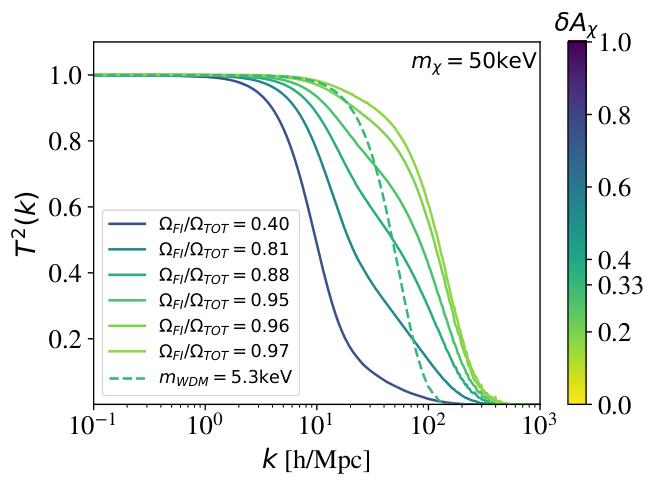
In the case of FIMPs from the FI and SW production mechanisms, the transfer function can take multiple forms. In the right panel of Fig. 2, we illustrate the transfer functions computed with class from the distributions shown in the left panel. They correspond to different benchmark scenarios all giving rise to $\Omega_{\chi}h^{2}=0.12$ within the top-philic DM model described in Sec. 4. Each benchmark has a different FI relative contribution to the total DM relic abundance ranging from 40% (dark purple) to 97% (light green). This is visible in the left panel as the FI contribution to the DM distribution function, that peaks around $q=2.5$, increases in amplitude when going from the dark purple to the light green curve. In the right panel, we see that when e.g. the FI contribution tends to 100%, the FIMP transfer function recovers the shape of a thermal WDM transfer function, depicted with a dashed curve for $m^{\mathrm{Ly}\alpha}_{\rm WDM}=5.3$ keV. This has already been pointed out in earlier works, see [30, 31]. Similarly, for 100% SW contribution, the FIMP transfer function resembles a WDM-like shape. For intermediate relative FI or SW contribution though, the shape of the transfer function can strongly deviate from thermal WDM like scenarios.

Using our modified class version, we have checked that the transfer function of eq. (3.6) provides a very good fit to the case of DM produced purely through the FI or SW mechanisms. For the fitting curves using $\mu=1.12$, as in the thermal WDM case, we obtain

where the parameter dependency of the breaking scales was inspired by the analytic estimate of the Lyman-$\alpha$ bound of eq. (3.2). The numerical prefactors in eqs. (3.8) and (3.9), on the other hand, have been obtained by doing a one-parameter fit based on the actual transfer functions produced by class. In the case of FI, the fit was done over 15 models, with a final error on the prefactors of $\sim 1.5\%$. In the case of SW, we used 20 models for the fit, with an expected error of $\sim 2\%$. In both cases, the fit has been optimised in the mass range where we expect the Lyman-$\alpha$ constraints to appear, based on eq. (3.1) (see App. C for further discussions).

In similar spirit to what was done in e.g. [37], we can now compare the breaking scales ($\alpha_{\mathrm{FI}}$ and $\alpha_{\mathrm{SW}}$) found in eqs. (3.8) and (3.9) with the breaking scale for WDM ($\alpha_{\mathrm{WDM}}$) from eq. (3.7), to obtain approximate Lyman-$\alpha$ bounds on FIMP DM. Assuming once more that the DM is produced at 100% through the FI or SW mechanisms and that this accounts for all of the DM abundance, taking the stringent WDM limit $m_{\rm WDM}^{\mathrm{Ly}\alpha}=5.3$ keV from [7] we get $m_{\rm FI}^{\rm lim}=15$ keV and $m_{\rm SW}^{\rm lim}=3.9$ keV in eq (3.1), see the second line of Tab. 1. We can see that these bounds are in very good agreement with the approximate constraints found in Sec. 3.1.1 using the rms velocity. When using the conservative bound of $m_{\rm WDM}^{\mathrm{Ly}\alpha}=1.9$ keV from [8] these prefactors reduce to $m_{\rm FI}^{\rm lim}=3.5$ keV and $m_{\rm SW}^{\rm lim}<1.0$ keV.

An alternative approach to extract the Lyman-$\alpha$ bounds on NCDM scenarios is based on the area criterion introduced in [25], see also [26, 32, 49]. The methodology goes as follows. For a given DM scenario $X$, the 3D power spectrum $P_{X}(k)$ has to be computed. The deviation from the corresponding CDM scenario is obtained by evaluating the ratio

where $P^{X}_{1\mathrm{D}}$ is the 1D power spectrum in the DM scenario $X$.

This ratio is estimated over the range of scales probed by the Lyman-$\alpha$ observations. In [25] the suggested range corresponding to the MIKE/HIRES+XQ-100 combined data set, used in [11] to derive the stringent WDM bound considered here, was taken to be

More precisely, in order to quantify the suppression of the power spectrum in the NCDM model $X$, one should compute the area estimator

and $A_{\rm CDM}=k_{\rm max}-k_{\rm min}$ by definition.

As underlined by the authors of the original work [25] introducing this criterion, let us emphasise that the area criterion has some arbitrariness in defining the integration limits, and should, therefore, only be used after careful calibration with an example WDM model. For the cosmological and precision parameters considered in our analysis, we get

A NCDM scenario that would give rise to $\delta A_{X}=\delta A_{\rm WDM}$ above is thus expected to saturate the stringent WDM Lyman-$\alpha$ bound considered here.⁸⁸ 8 Notice that in [25], a much smaller $\delta A_{\rm WDM}$ of 0.21 is reported for a 5.3 keV WDM. We have checked together with R. Murgia of [25] that the methodology followed here is perfectly correct. A discrepancy with the numerical results for $\delta A_{\rm WDM}$ quoted in [25] has also been reported in e.g. [32]. This emphasises the importance of recomputing self-consistently the $\delta A_{\rm WDM}$ before applying any constraint to a new NCDM scenario.

Making use of the linear 3D power spectrum computed with our modified version of class  for pure FI and SW DM scenarios and, comparing $\delta A_{\mathrm{FI,\,dec}}$ and $\delta A_{\rm SW}$ to the stringent bound provided by eq. (3.13), we get a limit similar to the one derived in Secs. 3.1.1 and 3.1.2. More precisely, for the prefactors of eq. (3.1), we get $m_{\rm FI}^{\rm lim}=15$ keV⁹⁹ 9 Note that if we make use of the perfect fluid approximation in class, we obtain $m_{\rm FI}^{\rm lim}=16$ keV, as in [32]. However, we will switch this approximation off for NCDM from FI, see App. C. and $m_{\rm SW}^{\rm lim}=3.8$ keV, see the third line of Tab. 1. We have also checked that using the fits provided in eqs. (3.8) and (3.9) instead of the $P(k)$ from class gives rise to the same conclusions. It appears, therefore, that in the case of pure FI or SW, all 3 methodologies considered in Sec. 3.1 agree with each other. In particular, this suggests that a very accurate estimate of the Lyman-$\alpha$ bound, for FIMP scenarios with unimodal distribution functions, can readily be extracted from eq. (3.2) without going through the detailed implementation of the NCDM model in class. In contrast, a more advanced approach proposed in [48], where a Lyman-$\alpha$ likelihood was developed for multiple NCDM models, allows for full Monte Carlo Markov Chain (MCMC) analyses. However, such analyses are hindered by the execution speed of the corresponding NCDM model in class. For the models considered here, the corresponding runtime needed to calculate the matter power spectrum is of the order of $\sim 30\,$min per model¹⁰¹⁰ 10 See App. C for more details on the computation time., making MCMC analyses computationally infeasible. As such, here we limit ourselves to the more simplistic methods discussed above.

In the case of mixed FI-SW scenarios, the DM distribution function is multimodal and the resulting transfer function can significantly deviate from the WDM one, as illustrated in Fig. 2. The area criterion is the only estimator of the Lyman-$\alpha$ bound that has been carefully tested against hydrodynamical simulations for a large ensemble of NCDM scenarios, see [25, 50]. For this reason, we make use of the latter criterion when considering mixed FI-SW models. In particular, for the set of benchmarks of Fig. 2, the gradient of colours in the curves corresponds to a value of the area criterion. More precisely, going from purple to green curves we have $\delta A_{\chi}=\left(0.75,0.54,0.38,0.29,0.20,0.18\right)$, respectively, i.e. the first three benchmarks are excluded when considering eq. (3.13). We have also checked that the area criterion gives rise to a more conservative bound than the estimator of eq. (3.4) for mixed scenarios. As a result, for mixed FI-SW scenarios, it necessary to implement the exact NCDM model in class in order to extract a reliable estimate of the Lyman-$\alpha$ bound.

References

- [1] Planck collaboration, N. Aghanim et al., Planck 2018 results. VI. Cosmological parameters, Astron. Astrophys. 641 (2020) A6, [1807.06209].
- [2] F. Kahlhoefer, Review of LHC Dark Matter Searches, Int. J. Mod. Phys. A 32 (2017) 1730006, [1702.02430].
- [3] T. Marrodán Undagoitia and L. Rauch, Dark matter direct-detection experiments, J. Phys. G 43 (2016) 013001, [1509.08767].
- [4] J. M. Gaskins, A review of indirect searches for particle dark matter, Contemp. Phys. 57 (2016) 496–525, [1604.00014].
- [5] M. Viel, J. Lesgourgues, M. G. Haehnelt, S. Matarrese and A. Riotto, Constraining warm dark matter candidates including sterile neutrinos and light gravitinos with WMAP and the Lyman-alpha forest, Phys. Rev. D 71 (2005) 063534, [astro-ph/0501562].
- [6] M. Viel, G. D. Becker, J. S. Bolton and M. G. Haehnelt, Warm dark matter as a solution to the small scale crisis: New constraints from high redshift Lyman- forest data, Phys. Rev. D 88 (2013) 043502, [1306.2314].
- [7] N. Palanque-Delabrouille, C. Yèche, N. Schöneberg, J. Lesgourgues, M. Walther, S. Chabanier et al., Hints, neutrino bounds and WDM constraints from SDSS DR14 Lyman- and Planck full-survey data, JCAP 04 (2020) 038, [1911.09073].
- [8] A. Garzilli, O. Ruchayskiy, A. Magalich and A. Boyarsky, How warm is too warm? Towards robust Lyman- forest bounds on warm dark matter, 1912.09397.
- [9] S. Ikeuchi, Galaxy formation theory and large scale structure in the universe, in Workshop on Grand Unified Theories and Cosmology, 1986.
- [10] M. J. Rees, Lyman absorption lines in quasar spectra: evidence for gravitationally-confined gas in dark minihaloes, Mon. Not. R. Astron. Soc. 218 (01, 1986) 25P–30P.
- [11] V. Iršič et al., New Constraints on the free-streaming of warm dark matter from intermediate and small scale Lyman- forest data, Phys. Rev. D96 (2017) 023522, [1702.01764].
- [12] M. Bolz, A. Brandenburg and W. Buchmuller, Thermal production of gravitinos, Nucl. Phys. B 606 (2001) 518–544, [hep-ph/0012052].
- [13] J. Pradler and F. D. Steffen, Constraints on the Reheating Temperature in Gravitino Dark Matter Scenarios, Phys. Lett. B 648 (2007) 224–235, [hep-ph/0612291].
- [14] J. McDonald, Thermally generated gauge singlet scalars as selfinteracting dark matter, Phys. Rev. Lett. 88 (2002) 091304, [hep-ph/0106249].
- [15] L. Covi, L. Roszkowski and M. Small, Effects of squark processes on the axino CDM abundance, JHEP 07 (2002) 023, [hep-ph/0206119].
- [16] T. Asaka, K. Ishiwata and T. Moroi, Right-handed sneutrino as cold dark matter, Phys. Rev. D 73 (2006) 051301, [hep-ph/0512118].
- [17] J. M. Frere, F. S. Ling, L. Lopez Honorez, E. Nezri, Q. Swillens and G. Vertongen, MeV right-handed neutrinos and dark matter, Phys. Rev. D 75 (2007) 085017, [hep-ph/0610240].
- [18] L. J. Hall, K. Jedamzik, J. March-Russell and S. M. West, Freeze-In Production of FIMP Dark Matter, JHEP 03 (2010) 080, [0911.1120].
- [19] L. Covi, J. E. Kim and L. Roszkowski, Axinos as cold dark matter, Phys. Rev. Lett. 82 (1999) 4180–4183, [hep-ph/9905212].
- [20] J. L. Feng, A. Rajaraman and F. Takayama, SuperWIMP dark matter signals from the early universe, Phys. Rev. D 68 (2003) 063504, [hep-ph/0306024].
- [21] D. Blas, J. Lesgourgues and T. Tram, The Cosmic Linear Anisotropy Solving System (CLASS) II: Approximation schemes, JCAP 07 (2011) 034, [1104.2933].
- [22] J. Lesgourgues and T. Tram, The Cosmic Linear Anisotropy Solving System (CLASS) IV: efficient implementation of non-cold relics, JCAP 1109 (2011) 032, [1104.2935].
- [23] K. J. Bae, A. Kamada, S. P. Liew and K. Yanagi, Light axinos from freeze-in: production processes, phase space distributions, and Ly- forest constraints, JCAP 1801 (2018) 054, [1707.06418].
- [24] P. Bode, J. P. Ostriker and N. Turok, Halo formation in warm dark matter models, Astrophys. J. 556 (2001) 93–107, [astro-ph/0010389].
- [25] R. Murgia, A. Merle, M. Viel, M. Totzauer and A. Schneider, ”Non-cold” dark matter at small scales: a general approach, JCAP 1711 (2017) 046, [1704.07838].
- [26] A. Schneider, Astrophysical constraints on resonantly produced sterile neutrino dark matter, JCAP 04 (2016) 059, [1601.07553].
- [27] M. Garny and J. Heisig, Interplay of super-WIMP and freeze-in production of dark matter, Phys. Rev. D 98 (2018) 095031, [1809.10135].
- [28] J. Harz and K. Petraki, Radiative bound-state formation in unbroken perturbative non-Abelian theories and implications for dark matter, JHEP 07 (2018) 096, [1805.01200].
- [29] J. Heeck and D. Teresi, Cold keV dark matter from decays and scatterings, Phys. Rev. D96 (2017) 035018, [1706.09909].
- [30] S. Boulebnane, J. Heeck, A. Nguyen and D. Teresi, Cold light dark matter in extended seesaw models, JCAP 1804 (2018) 006, [1709.07283].
- [31] G. Ballesteros, M. A. G. Garcia and M. Pierre, How warm are non-thermal relics? Lyman- bounds on out-of-equilibrium dark matter, JCAP 03 (2021) 101, [2011.13458].
- [32] F. D’Eramo and A. Lenoci, Lower mass bounds on FIMP dark matter produced via freeze-in, JCAP 10 (2021) 045, [2012.01446].
- [33] G. Bélanger, F. Boudjema, A. Goudelis, A. Pukhov and B. Zaldivar, micrOMEGAs5.0 : Freeze-in, Comput. Phys. Commun. 231 (2018) 173–186, [1801.03509].
- [34] G. Bélanger, C. Delaunay, A. Pukhov and B. Zaldivar, Dark matter abundance from the sequential freeze-in mechanism, Phys. Rev. D 102 (2020) 035017, [2005.06294].
- [35] T. Binder, T. Bringmann, M. Gustafsson and A. Hryczuk, Early kinetic decoupling of dark matter: when the standard way of calculating the thermal relic density fails, Phys. Rev. D 96 (2017) 115010, [1706.07433].
- [36] P. Gondolo and G. Gelmini, Cosmic abundances of stable particles: Improved analysis, Nucl. Phys. B 360 (1991) 145–179.
- [37] I. Baldes, Q. Decant, D. C. Hooper and L. Lopez-Honorez, Non-Cold Dark Matter from Primordial Black Hole Evaporation, JCAP 08 (2020) 045, [2004.14773].
- [38] A. Merle and M. Totzauer, keV Sterile Neutrino Dark Matter from Singlet Scalar Decays: Basic Concepts and Subtle Features, JCAP 1506 (2015) 011, [1502.01011].
- [39] S. Baumholzer, V. Brdar, P. Schwaller and A. Segner, Shining Light on the Scotogenic Model: Interplay of Colliders and Cosmology, JHEP 09 (2020) 136, [1912.08215].
- [40] C. Dvorkin, T. Lin and K. Schutz, Making dark matter out of light: freeze-in from plasma effects, Phys. Rev. D 99 (2019) 115009, [1902.08623].
- [41] C. Dvorkin, T. Lin and K. Schutz, Cosmology of Sub-MeV Dark Matter Freeze-In, Phys. Rev. Lett. 127 (2021) 111301, [2011.08186].
- [42] S. Ikeuchi, The baryon clump within an extended dark matter region, Astrophysics and Space Science 118 (Jan, 1986) 509–514.
- [43] M. J. Rees, Lyman absorption lines in quasar spectra: evidence for gravitationally-confined gas in dark minihaloes, Monthly Notices of the Royal Astronomical Society 218 (01, 1986) 25P–30P.
- [44] S. Colombi, S. Dodelson and L. M. Widrow, Large scale structure tests of warm dark matter, Astrophys. J. 458 (1996) 1, [astro-ph/9505029].
- [45] K. Jedamzik, M. Lemoine and G. Moultaka, Gravitino, axino, Kaluza-Klein graviton warm and mixed dark matter and reionisation, JCAP 07 (2006) 010, [astro-ph/0508141].
- [46] J. Baur, N. Palanque-Delabrouille, C. Yeche, A. Boyarsky, O. Ruchayskiy, E. Armengaud et al., Constraints from Ly- forests on non-thermal dark matter including resonantly-produced sterile neutrinos, JCAP 12 (2017) 013, [1706.03118].
- [47] R. Murgia, V. Irˇsič and M. Viel, Novel constraints on noncold, nonthermal dark matter from Lyman- forest data, Phys. Rev. D 98 (2018) 083540, [1806.08371].
- [48] M. Archidiacono, D. C. Hooper, R. Murgia, S. Bohr, J. Lesgourgues and M. Viel, Constraining Dark Matter-Dark Radiation interactions with CMB, BAO, and Lyman-, JCAP 10 (2019) 055, [1907.01496].
- [49] D. Egana-Ugrinovic, R. Essig, D. Gift and M. LoVerde, The Cosmological Evolution of Self-interacting Dark Matter, JCAP 05 (2021) 013, [2102.06215].
- [50] R. Murgia, Constraining Dark Matter properties with the Inter-Galactic Medium and other probes, Ph.D. thesis, SISSA, Trieste, 9, 2019.
- [51] M. Hufnagel, K. Schmidt-Hoberg and S. Wild, BBN constraints on MeV-scale dark sectors. Part I. Sterile decays, JCAP 02 (2018) 044, [1712.03972].
- [52] C. Pitrou, A. Coc, J.-P. Uzan and E. Vangioni, Precision big bang nucleosynthesis with improved Helium-4 predictions, Phys. Rept. 754 (2018) 1–66, [1801.08023].
- [53] Particle Data Group collaboration, C. Patrignani, K. Agashe, G. Aielli, C. Amsler, M. Antonelli, D. M. Asner et al., Review of Particle Physics, 2016-2017, Chin. Phys. C 40 (2016) 100001. 1808 p.
- [54] S.-P. Li, X.-Q. Li, X.-S. Yan and Y.-D. Yang, Simple estimate of BBN sensitivity to light freeze-in dark matter, Phys. Rev. D 104 (2021) 115007, [2106.07122].
- [55] G. Belanger, F. Boudjema, C. Hugonie, A. Pukhov and A. Semenov, Relic density of dark matter in the NMSSM, JCAP 09 (2005) 001, [hep-ph/0505142].
- [56] A. Ibarra, A. Ringwald and C. Weniger, Hidden gauginos of an unbroken U(1): Cosmological constraints and phenomenological prospects, JCAP 01 (2009) 003, [0809.3196].
- [57] G. Bélanger et al., LHC-friendly minimal freeze-in models, JHEP 02 (2019) 186, [1811.05478].
- [58] L. Calibbi, F. D’Eramo, S. Junius, L. Lopez-Honorez and A. Mariotti, Displaced new physics at colliders and the early universe before its first second, JHEP 05 (2021) 234, [2102.06221].
- [59] G. Arcadi and L. Covi, Minimal Decaying Dark Matter and the LHC, JCAP 08 (2013) 005, [1305.6587].
- [60] G. Arcadi, L. Covi and F. Dradi, LHC prospects for minimal decaying Dark Matter, JCAP 10 (2014) 063, [1408.1005].
- [61] A. Ibarra, A. Pierce, N. R. Shah and S. Vogl, Anatomy of Coannihilation with a Scalar Top Partner, Phys. Rev. D 91 (2015) 095018, [1501.03164].
- [62] M. Garny, J. Heisig, M. Hufnagel and B. Lülf, Top-philic dark matter within and beyond the WIMP paradigm, Phys. Rev. D 97 (2018) 075002, [1802.00814].
- [63] A. Sommerfeld, Über die Beugung und Bremsung der Elektronen, Annals Phys. 403 (1931) 257–330.
- [64] J. Hisano, S. Matsumoto and M. M. Nojiri, Unitarity and higher order corrections in neutralino dark matter annihilation into two photons, Phys. Rev. D67 (2003) 075014, [hep-ph/0212022].
- [65] M. Cirelli, A. Strumia and M. Tamburini, Cosmology and Astrophysics of Minimal Dark Matter, Nucl. Phys. B787 (2007) 152–175, [0706.4071].
- [66] S. P. Liew and F. Luo, Effects of QCD bound states on dark matter relic abundance, JHEP 02 (2017) 091, [1611.08133].
- [67] A. Mitridate, M. Redi, J. Smirnov and A. Strumia, Cosmological Implications of Dark Matter Bound States, JCAP 05 (2017) 006, [1702.01141].
- [68] S. Biondini and M. Laine, Thermal dark matter co-annihilating with a strongly interacting scalar, JHEP 04 (2018) 072, [1801.05821].
- [69] F. Ambrogi, C. Arina, M. Backovic, J. Heisig, F. Maltoni, L. Mantani et al., MadDM v.3.0: a Comprehensive Tool for Dark Matter Studies, Phys. Dark Univ. 24 (2019) 100249, [1804.00044].
- [70] T. Binder, Refining the chemical and kinetic decoupling description of thermally produced dark matter, Ph.D. thesis, Gottingen U., 2019.
- [71] S. Biondini and J. Ghiglieri, Freeze-in produced dark matter in the ultra-relativistic regime, JCAP 03 (2021) 075, [2012.09083].
- [72] G. Jackson and M. Laine, Efficient numerical integration of thermal interaction rates, JHEP 09 (2021) 125, [2107.07132].
- [73] ATLAS collaboration, M. Aaboud et al., Search for heavy charged long-lived particles in the ATLAS detector in 36.1 fb-1 of proton-proton collision data at TeV, Phys. Rev. D 99 (2019) 092007, [1902.01636].
- [74] ATLAS collaboration, M. Aaboud et al., Search for long-lived, massive particles in events with displaced vertices and missing transverse momentum in = 13 TeV collisions with the ATLAS detector, Phys. Rev. D 97 (2018) 052012, [1710.04901].
- [75] W. Beenakker, C. Borschensky, M. Krämer, A. Kulesza and E. Laenen, NNLL-fast: predictions for coloured supersymmetric particle production at the LHC with threshold and Coulomb resummation, JHEP 12 (2016) 133, [1607.07741].
- [76] K. Jedamzik, Big bang nucleosynthesis constraints on hadronically and electromagnetically decaying relic neutral particles, Phys. Rev. D 74 (2006) 103509, [hep-ph/0604251].
- [77] M. Kawasaki, K. Kohri, T. Moroi and Y. Takaesu, Revisiting Big-Bang Nucleosynthesis Constraints on Long-Lived Decaying Particles, Phys. Rev. D 97 (2018) 023502, [1709.01211].
- [78] K. Jedamzik, Bounds on long-lived charged massive particles from Big Bang nucleosynthesis, JCAP 03 (2008) 008, [0710.5153].
- [79] M. Kusakabe, T. Kajino, T. Yoshida and G. J. Mathews, Effect of Long-lived Strongly Interacting Relic Particles on Big Bang Nucleosynthesis, Phys. Rev. D 80 (2009) 103501, [0906.3516].
- [80] P. F. Depta, M. Hufnagel and K. Schmidt-Hoberg, ACROPOLIS: A generiC fRamework fOr Photodisintegration Of LIght elementS, JCAP 03 (2021) 061, [2011.06518].
- [81] A. Arbey, AlterBBN: A program for calculating the BBN abundances of the elements in alternative cosmologies, Comput. Phys. Commun. 183 (2012) 1822–1831, [1106.1363].
- [82] ATLAS collaboration, M. Aaboud et al., Search for heavy charged long-lived particles in proton-proton collisions at TeV using an ionisation measurement with the ATLAS detector, Phys. Lett. B 788 (2019) 96–116, [1808.04095].
- [83] CMS collaboration, A. M. Sirunyan et al., Search for long-lived particles using nonprompt jets and missing transverse momentum with proton-proton collisions at 13 TeV, Phys. Lett. B 797 (2019) 134876, [1906.06441].
- [84] M. R. Mosbech, C. Boehm, S. Hannestad, O. Mena, J. Stadler and Y. Y. Y. Wong, The full Boltzmann hierarchy for dark matter-massive neutrino interactions, JCAP 03 (2021) 066, [2011.04206].