Matroid-Based TSP Rounding for Half-Integral Solutions
Abstract
We show how to round any half-integral solution to the subtour-elimination relaxation for the TSP, while losing a less-than-1.5 factor. Such a rounding algorithm was recently given by Karlin, Klein, and Oveis Gharan based on sampling from max-entropy distributions. We build on an approach of Haddadan and Newman to show how sampling from the matroid intersection polytope, and a new use of max-entropy sampling, can give better guarantees.
1 Introduction
The (symmetric) traveling salesman problem asks: given an graph with edge-lengths , find the shortest tour that visits all vertices at least once. The Christofides-Serdyukov algorithm [Chr76, Ser78] gives a -approximation to this APX-hard problem; this was recently improved to a -approximation by the breakthrough work of Karlin, Klein, and Oveis Gharan, where [KKO20b]. A related question is: what is the integrality gap of the subtour-elimination polytope relaxation for the TSP? Wolsey had adapted the Christofides-Serdyukov analysis to show an upper bound of [Wol80] (also [SW90]), and there exists a lower bound of . Building on their above-mentioned work, Karlin, Klein, and Oveis Gharan gave an integrality gap of for another small constant [KKO21], thereby making the first progress towards the conjectured optimal value of in nearly half a century.
Both these recent results are based on a randomized version of the Christofides-Serdyukov algorithm proposed by Oveis Gharan, Saberi, and Singh [OSS11]. This algorithm first samples a spanning tree (plus perhaps one edge) from the max-entropy distribution with marginals matching the LP solution, and adds an -join on the odd-degree vertices in it, thereby getting an Eulerian spanning subgraph. Since the first step has expected cost equal to that of the LP solution, these works then bound the cost of this -join by strictly less than half the optimal value, or the LP value. The proof uses a cactus-like decomposition of the min-cuts of the graph with respect to the values , like in [OSS11].
Given the barrier has been broken, we can ask: what other techniques can be effective here? How can we make further progress? These questions are interesting even for cases where the LP has additional structure. The half-integral cases are particularly interesting due to the Schalekamp, Williamson, and van Zuylen conjecture, which says that the integrality gap is achieved on instances where the LP has optimal half-integral solutions [SWvZ14]. The team of Karlin, Klein, and Oveis Gharan first used their max-entropy approach to get an integrality gap of for half-integral LP solutions [KKO20a], before they moved on to the general case in [KKO20b] and obtained an integrality gap of ; the latter improvement is considerably smaller than in the half-integral case. It is natural to ask: can we do better for half-integral instances?
In this paper, we answer this question affirmatively. We show how to get tours of expected cost at most times the linear program value using an algorithm based on matroid intersection. Moreover, some of these ideas can be used to strengthen the max-entropy sampling approach in the half-integral case. The matroid intersection approach and the strengthened max-entropy approach each yield improvements over the bound in [KKO20a]. Combining the techniques gives our final quantitative improvement:
Theorem 1.1.
Let be a half-integral solution to the subtour elimination polytope with cost . There is a randomized algorithm that rounds to an integral solution whose cost is at most , where .
We view our work as showing a proof-of-concept of the efficacy of combinatorial techniques (matroid intersection, and flow-based charging arguments) in getting an improvement for the half-integral case. We hope that these techniques, ideally combined with max-entropy sampling techniques, can give further progress on this central problem.
Our Techniques
The algorithm is again in the Christofides-Serdyukov framework. It is easiest to explain for the case where the graph (a) has an even number of vertices, and (b) has no (non-trivial) proper min-cuts with respect to the LP solution values —specifically, the only sets for which correspond to the singleton cuts. Here, our goal is that each edge is “even” with some probability: i.e., both of its endpoints have even degree with probability . In this case we use an idea due to Haddadan and Newman [HN19]: we shift and get a -valued solution to the subtour elimination polytope . Specifically, we find a random perfect matching in the support of , and set for , and otherwise, thereby ensuring . To pick a random tree from this shifted distribution , we do one of the following:
- 1.
We pick a random “independent” set of matching edges (so that no edge in is incident to two edges of ). For each , we place partition matroid constraints enforcing that exactly one edge is picked at each endpoint—which, along with itself, gives degree and thereby makes the edge even as desired. Finding spanning trees subject to another matroid constraint can be implemented using matroid intersection.
- 2.
Or, instead we sample a random spanning tree from the max-entropy distribution, with marginals being the shifted value . (In contrast, [KKO20a] sample trees from itself; our shifting allows us to get stronger notions of evenness than they do: e.g., we can show that every edge is “even-at-last” with constant probability, as opposed to having at least one even-at-last edge in each tight cut with some probabiltiy.)
(Our algorithm randomizes between the two samplers to achieve the best guarantees.) For the -join step, it suffices to give fractional values to edges so that for every odd cut in , the -mass leaving the cut is at least 1. In the special case we consider, each edge only participates in two min-cuts—those corresponding to its two endpoints. So set if is even, and if not; the only cuts with are minimum cuts, and these cuts will not show up as -join constraints, due to evenness. For this setting, if an edge is even with probability , we get a -approximation!
It remains to get rid of the two simplifying assumptions. To sample trees when is odd (an open question from [HN19]), we add a new vertex to fix the parity, and perform local surgery on the solution to get a new TSP solution and reduce to the even case. The challenge here is to show that the losses incurred are small, and hence each edge is still even with constant probability.
Finally, what if there are proper tight sets , i.e., where ? We use the cactus decomposition of a graph (also used in [OSS11, KKO20a]) to sample spanning trees from pieces of with no proper min-cuts, and stitch these trees together. These pieces are formed by contracting sets of vertices in , and have a hierachical structure. Moreover, each such piece is either of the form above (a graph with no proper min-cuts) for which we have already seen samplers, or else it is a double-edged cycle (which is easily sampled from). Since each edge may now lie in many min-cuts, we no longer just want an edge to have both endpoints be even. Instead, we use an idea from [KKO20a] that uses the hierarchical structure on the pieces considered above. Every edge of the graph is “settled” at exactly one of these pieces, and we ask for both of its endpoints to have even degree in the piece at which it is settled. The value of such an edge may be lowered in the -join without affecting constraints corresponding to cuts in the piece at which it is settled.
Since cuts at other levels of the hierarchy may now be deficient because of the lower values of , we may need to increase the values for other “lower” edges to satisfy these deficient cuts. This last part requires a charging argument, showing that each edge has that is strictly smaller than in expectation. For our samplers, the naïve approach of distributing charge uniformly as in [KKO20a] does not work, so we instead formulate this charging as a flow problem.
2 Notation and Preliminaries
Given a multigraph , and a set , let denote the cut consisting of the edges connecting to ; and are called shores of the cut. (For a singleton set , we write instead of .) A subset is proper if ; a cut is called proper if the set is a proper subset. A set is tight if equals the size of the minimum edge-cut in . Two sets and are crossing if , , , and are all non-empty.
Define the subtour elimination polytope :
| (LP-TSP) | ||||
Let be half-integral and feasible for (LP-TSP). W.l.o.g. we can focus on solutions with for each , doubling edges if necessary. The support graph is then a -regular -edge-connected (henceforth 4EC) multigraph.
The spanning tree polytope for a multigraph is:
| (LP-spT) | ||||
where is the set of edges with both endpoints in . This is the graphic matroid polytope, and the convex hull of the spanning trees.
Definition 2.1 (-Trees).
Given a multigraph and “root” vertex , an -tree is a connected subgraph with edges: the vertex has degree exactly , and the subgraph restricted to the other vertices is a spanning tree on them. This is a matroid, though we do not use this fact.
The (integral) perfect matching polytope is defined as follows:
| (LP-PM) | ||||
The (integral) -join dominator polytope is defined as follows. Let , even.
Fact 2.2.
For any solution , it holds that , (when is even), and for , even.
Lemma 2.3.
Consider a sub-partition of the edge set of . Let be a fractional solution to (LP-spT) that satisfies for all . Then we can efficiently sample from a probability distribution over spanning trees which contain at most one edge from each of the parts , such that .
Proof.
This follows from the integrality of the matroid intersection polytope. ∎
2.1 The Max-Entropy Distribution over Spanning Trees
Definition 2.4 (Strong Rayleigh Distributions, [BBL09]).
Let be a probability distribution on spanning trees. The generating polynomial for is . We say is strongly Rayleigh (SR) if is a real stable polynomial (i.e., if lies in the upper half plane).
A distribution over spanning trees is called or weighted uniform if there exist non-negative weights such that . Borcea et al. [BBL09] showed that -uniform spanning tree distributions are SR.
Theorem 2.5 ([OSS11]).
There exists a -uniform distribution over spanning trees such that given in the spanning tree polytope of ,
The max-entropy distribution, which is the distribution on spanning trees maximizing the entropy of subject to preserving the marginals (that is, ), is one such distribution.
Asadpour et al [AGM+17] showed that we can find weights which approximately respect the marginals given by a vector in the spanning tree polytope in polynomial time.
Theorem 2.6 ([AGM+17]).
Given in the spanning tree polytope of and some , values for can be found such that, for all , the -uniform distribution satisfies
The running time is polynomial in and .
Fact 2.7 ([BBL09]).
Let be an SR distribution. Let be a subset of edges. Then the projection of onto , i.e., , is also SR. Moreover, for any edge , conditioning on or on preserves the SR property.
Theorem 2.8 (Negative Correlation, [OSS11]).
Let be an SR distribution on spanning trees.
- 1.
Let be a set of edges and , where . Then, , where the are independent Bernoulli random variables with success probabilities and .
- 2.
For any set of edges and ,
- (i)
, and
- (ii)
.
- (i)
Theorem 2.9 ([Hoe56], Corollary 2.1).
Let and let . Let be Bernoulli random variables with probabilities that maximize (or minimize) over all possible success probabilities for for which . Then for some .
3 Samplers
In this section, we describe the MaxEnt and MatInt samplers for graphs that contain no proper min-cuts. We give bounds on certain correlations between edges that will be used in §5 to prove that every edge is “even” with constant probability. The samplers for the case where the graph has an odd number of vertices are more technical and are deferred to Appendix B.
Suppose the graph is 4-regular and 4-edge-connected (4EC), contains at least four vertices, and has no proper min-cuts.11 1 This implies that is a simple graph: since parallel edges between means that is a proper min-cut; we use this simplicity of the graph often in the arguments of this section. This means all proper cuts have six or more edges. We are given a dedicated external vertex ; the vertices that are not external are called internal. (In future sections, this vertex will be given by a cut hierarchy.) Call the edges in external edges; all other edges are internal. An internal vertex is called a boundary vertex if it is adjacent to . An edge is said to be special if both of its endpoints are non-boundary vertices.
We show two ways to sample a spanning tree on , the graph induced on the internal vertices, being faithful to the marginals , i.e., for all . Moreover, we want that for each internal edge, both its endpoints have even degree in with constant probability. This property will allow us to lower the cost of the -join in §6. While both samplers will satisfy this property, each will do better in certain cases. The MatInt sampler targets special edges; it allows us to randomly “hand-pick” edges of this form and enforce that both of its endpoints have degree 2 in the tree. The MaxEnt sampler, on the other hand, relies on maximizing the randomness of the spanning tree sampled (subject to being faithful to the marginals); negative correlation properties allow us to obtain the evenness property, and in particular, better probabilities than MatInt for non-special edges, and a worse probability for the special edges.
Our samplers will depend on the parity of : when is even, the MatInt sampler is the one given by [HN19, Theorem 13], which we describe in §3.1. They left the case of odd as an open problem, and in Appendix B we extend their procedure to the odd case.
3.1 Samplers for Even
Since is -regular and 4EC and is even, setting a value of on each edge gives a solution to the perfect matching polytope by 2.2.
- 1.
Sample a perfect matching such that for all .
- 2.
(Shift) Define a new fractional solution (that depends on ): set for , and otherwise. We have (and hence by 2.2): indeed, each vertex has because is a perfect matching. Moreover, every proper cut in has at least six edges, so . Furthermore,
(1) - 3.
Sample a spanning tree faithful to the marginals , using one of two samplers:
- (a)
MaxEnt Sampler: Sample from the max-entropy distribution on spanning trees with marginals .
- (b)
MatInt Sampler:
- i.
Color the edges of using colors such that no edge of is adjacent to two edges of having the same color; e.g., by greedily -coloring the -regular graph . Let be one of these color classes picked uniformly at random. Hence, , and .
- ii.
For each edge , let and be the sets of edges incident at and other than . Note that . Place partition matroid constraints and on each of these sets. Finally, restrict the partition constraints to the internal edges of ; this means some of these constraints are no longer tight for the solution .
- i.
- (c)
Given the sub-matching , and the partition matroid on the internal edges defined using , use Lemma 2.3 to sample a tree on (i.e., on the internal vertices and edges of ) with marginals , subject to this partition matroid .
- (a)
Conditioned on the matching , we have ; now using (1), we have for all .

3.2 Correlation Properties of Samplers
Let be a tree sampled using either the MatInt or the MaxEnt sampler. The following claims will be used to prove the evenness property in §5. Each table gives lower bounds on the corresponding probabilities for each sampler. The proofs for odd are in Appendix B.
Lemma 3.1.
If are internal edges incident to a vertex , then
| Probability Statement | MatInt | MaxEnt |
|---|---|---|
Lemma 3.2.
If edges incident to a vertex are all internal, then
| Probability Statement | MatInt | MaxEnt |
|---|---|---|
Lemma 3.3.
For an internal edge :
- (a)
if both endpoints are non-boundary vertices, then
Probability Statement MatInt MaxEnt - (b)
if both are boundary vertices, then
Probability Statement MatInt MaxEnt exactly one of has odd degree in
3.2.1 Correlation Properties: even
We now prove the correlation properties for the even case: the numerical bounds for the even case are better than those claimed above (which will be dictated by the proofs of the odd case; see Appendix B).
Proof of Lemma 3.1, Even Case.
To prove , we need only knowledge of the marginals and not the specific sampler. If one of lies in (which happens w.p. ), then its -value equals and it belongs to w.p. , and the other edge is chosen w.p. , making the unconditional probability . Similarly, conditioned on lying in and hence belonging to , edge is not chosen w.p. , so .
The MaxEnt claim: It remains to show that . Conditioned on , we have w.p. . Now condition on neither nor in (happens w.p. ). By Theorem 2.8,
By Theorem 2.9, , so . Putting all of this together, we get
Proof of Lemma 3.2, Even Case.
The MatInt claims: Each perfect matching contains one of these four edges in . Say that edge is . If also belongs to (w.p. ), then contains exactly one of . Since , this gives us the first bound in Lemma 3.2. Moreover, the probability of this edge in belonging to the other pair (in this case, ) is . Hence , giving us the other bound in Lemma 3.2 for the MatInt sampler.
The MaxEnt claims: For the first bound in Lemma 3.2, we have that one of the four edges must be in and have -value 1. W.l.o.g., call that edge . The other three, , will be -valued edges. Since , we may apply Theorem 2.9 and obtain a lower bound of
For the second bound in Lemma 3.2, call and . W.l.o.g., we once again label . Then, . So for , we condition on . Then by Theorem 2.8,
Hence, we use Theorem 2.9 again and obtain . In total, we obtain
Proof of Lemma 3.3a, Even Case.
The MatInt claims: The event happens when , which happens w.p. , which is at least .
The MaxEnt claims: Condition on . Let and . Denote . Lower bound using Theorem 2.9: , so Consider the distribution over the edges in conditioned on ; this distribution is also SR. By Theorem 2.8, Applying Theorem 2.8 twice more,
By Theorem 2.9, . Using symmetry, we obtain ∎
Proof of Lemma 3.3b, Even Case.
The MatInt claims: For part (b), suppose (w.p. ), then each of have two other internal edges, each with -value . Let us say the good cases are when exactly one of these four is chosen; exactly one of has degree and the other has degree in these cases. We cannot choose zero of these four edges, because of the connectivity of , so all bad cases choose at least two of these four. Given the -values of on all four edges, the expected number of these edges chosen are , so the the probability of a bad case at most . This means that with probability at least , exactly one of has odd degree in . Since , we have proven (b).
The MaxEnt claims: Observe that the edge will always contribute either: 0 to both the degree of in and the degree of in OR 1 to both of these degrees. Let be the two internal edges incident to and be the two edges incident to .
- 1.
Case 1: . This implies are all -valued edges, so . Note that we must have . Therefore, .
- 2.
Case 2: , exactly two of are in . W.l.o.g., say , so and are in . , which implies (by Theorem 2.9) that .
- 3.
Case 3: , exactly one of is in . W.l.o.g., say , so we have . We condition on , which happens w.p. . Since we sample a spanning tree on the internal vertices, this means that at least one of is in . W.l.o.g., say . So in order to bound the probability that the internal parities of are different, equivalently we would like to bound . Since , Theorem 2.9 implies that . So removing the conditioning on gives a lower bound of .
Taking the minimum of the bounds , and in the three cases gives
4 Sampling Algorithm for General Solutions; and Cut Hierarchy
Now that we can sample a spanning tree from a graph with no proper min-cuts, we introduce the algorithm to sample an -tree from a 4-regular, 4EC graph, perhaps with proper min-cuts.
4.1 The Algorithm
Assume that the graph has a set of three special vertices , with each pair and having a pair of edges between them. This is without loss of generality (used in line 18). Define a double cycle to be a cycle graph in which each edge is replaced by a pair of parallel edges, and call each such pair partner edges.
The sampling algorithm appears as Algorithm 1, and is very similar to that in [KKO20a]: they refer to the sets in line 4 as critical sets. Since is a 4-regular, 4EC graph at every stage of the algorithm, if or 3, then must be a cycle set, whereas if , then may be a degree or cycle set. The following two claims are proved in Appendix A.1, and show that Algorithm 1 is well-defined.
Claim 4.1.
The graph remaining at the end of the algorithm (line 18) is a double cycle.
Claim 4.2.
In every iteration in Algorithm 1, is either a double cycle or a graph with no proper min-cuts.
We will prove the following theorem in §6. This in turn gives Theorem 1.1.
Theorem 4.3.
Let be the -tree chosen from Algorithm 1, and be the set of odd degree vertices in . The expected cost of the minimum cost -join for is at most .
4.2 The Cut Hierarchy
Recall our ultimate goal is to create a low cost, feasible solution in the -join polytope, where is the set of odd degree vertices in our sampled tree . We start with the fractional solution and then reduce the value of some edges. In the process, we may violate some constraints corresponding to min-cuts. To fix these cuts, we need a complete description of the min-cuts of a graph. This is achieved by the implicit hierarchy of critical sets that Algorithm 1 induces.
The hierarchy is given by a rooted tree .22 2 Since there are several graphs under consideration, the vertex set of is called . Moreover, for clarity, we refer to elements of as vertices, and elements of as nodes. The vertex set corresponds to all critical sets found by the algorithm, along with a root node and leaf nodes representing the vertices in . If is a critical set, we label the node in with , where we view and not . The root node is labelled and each leaf nodes is labelled by the vertex in corresponding to it. Now we define the edge set . A node is a child of if and is the first superset of contracted after in the algorithm. In addition, the root node is a parent of all nodes corresponding to critical sets that are not strictly contained in any other critical set (i.e., the critical sets corresponding to the vertices in the graph from line 17 when the while loop terminates). Finally, each leaf node is a child of the smallest critical set that contains it (or if no critical set contains it, is a child of the root node). Thus by construction, vertex sets labelling the children of a node are a partition of the vertex set labelling that node. A node in is a cycle or degree node if the corresponding critical set labelling it is a cycle or degree set, respectively. We say the root node is a cycle node (since the graph in line 18 is a double cycle), and accordingly call a cycle set. (The leaf nodes are not labelled as degree or cycle nodes.)

Definition 4.4 (Local multigraph).
Let be a set labelling a node in . Define the local multigraph to be the following graph: take and contract the subsets of labelling the children of in down to single vertices and contract to a single vertex . Remove any self-loops. The vertex is called the external vertex; all other vertices are called internal vertices. An internal vertex is called a boundary vertex if it is adjacent to the external vertex. The edges in are called internal edges. Observe that is precisely the graph in line 5 of Algorithm 1 when is a critical set, and is a double cycle when .
Properties of :
- 1.
Let be a 4-regular, 4EC graph with associated hierarchy . Let be a set labelling a node in . If is a degree node in , then has at least five vertices and no proper min-cuts, and hence every proper cut in has at least 6 edges. If is a cycle node in , then is exactly a double cycle.
These follow from 4.2 and the equivalence between and .
- 2.
- 3.
For a degree set , the graph having no proper min-cuts implies that it has no parallel edges. In particular, no vertex has parallel edges to the external vertex in . Hence we get the following:
Corollary 4.5.
For a set labeling a non-leaf node in and any internal vertex : if is a cycle set then , and if is a degree set then .
Finally, we show how the hierarchy allows us to characterize the min-cut structure of . The cactus representation of min-cuts ([FF09]) is a compact representation of the min-cuts of a graph, and it can be constructed from the cut hierarchy; we defer the details to Appendix A.2. In turn we obtain the following complete characterization of the min-cuts of in terms of local multigraphs.
Claim 4.6.
Any min-cut in is either (a) for some node in , or (b) where is obtained as follows: for some cycle set in , is the union of vertices corresponding to some contiguous segment of the cycle .
5 Analysis Part I: The Even-at-Last Property
The proof of Theorem 4.3 proceeds in two parts:
- (1)
In this section, we show that each edge is “even-at-last” with constant probability. (This is an extension of the property that both of its endpoints have even degree.)
- (2)
Then we construct the fractional -join. As always, is a feasible join, but we show how to save a constant fraction of the LP value for an edge when it is even-at-last. This savings causes other cuts to be deficient, so other edges raise their values in response. However, a charging argument shows that the -value for an edge does decrease by a constant factor, in expectation. This argument appears in §6.
To address part (1), let us define a notion of evenness for every edge in . In the case where has no proper min-cuts, we called an edge even if both of its endpoints were even in . Now, the general definition of evenness will depend on where an edge belongs in the hierarchy .
Definition 5.1.
We say an edge is settled at if is the (unique) set such that is an internal edge of ; call the last set of . If is a degree or cycle set, we call a degree edge or cycle edge, respectively.
Definition 5.2 (Even-at-Last).
Let be the last set of , and be the restriction of to .
- 1.
A degree edge is called even-at-last (EAL) if both of its endpoints have even degree in .
- 2.
For a cycle edge , the graph is a chain of vertices , with consecutive vertices connected by two parallel edges. Let , and be the partition of this chain. The cuts and are called the canonical cuts for . Cycle edge is called even-at-last (EAL) if both canonical cuts are crossed an even number of times by ; in other words, if there is exactly one edge in from each of the two pairs of external partner edges leaving and .
Informally, a degree edge is EAL in the general case if it is even in the tree at the level at which it is settled. Also note that cycle edges settled at the same (cycle) set are either all EAL or none are EAL.
Definition 5.3 (Special and Half-Special Edges).
Let be settled at a degree set . We say that is special if both of its endpoints are non-boundary vertices in and half-special if exactly one of its endpoints is a boundary vertex in .
We now prove a key property used in §6 to reduce the -values of edges in the fractional -join.
Theorem 5.4 (The Even-at-Last Property).
The table below gives lower bounds on the probability that special, half-special, and all other types of degree edges are EAL in each of the two samplers.
| special | half-special | other degree edges | |
| MatInt | |||
| MaxEnt | |||
| - | - |
Moreover, a cycle edge is EAL w.p. at least .
Proof.
Let be settled at . Let be the spanning tree sampled on the internal vertices of (in the notation of Algorithm 1, the spanning tree sampled on ).
First, assume that is a degree set:
- 1.
If none of the endpoints of are boundary vertices in (i.e., is special), then it is EAL exactly when both its endpoints have even degree in . By Lemma 3.3(a), this happens w.p. for the MatInt sampler and w.p. for the MaxEnt sampler.
- 2.
Now suppose that is half-special, so that exactly one of the endpoints of (say ) is a boundary vertex in , with edge incident to leaving . By Lemma 3.2, the other endpoint is even in w.p. for the MatInt sampler and for the MaxEnt sampler. Moreover, the edge is chosen at a higher level than and is therefore independent of , and hence can make the degree of even w.p. . Thus is EAL w.p. for the MatInt sampler and for the MaxEnt sampler.
- 3.
Suppose both endpoints of are boundary vertices of , with edges leaving . Let be the probability that the degrees of vertices in the tree chosen within have the same parity, and . Now, when is contracted and we choose a -tree on the graph consistent with the marginals, let be the probability that either both or neither of are chosen in , and . Hence
(2) where and correspond to different parity combinations of and in and correspond to whether and are chosen in . The second inequality follows from D.1 applied to the random -tree .
- (a)
If are settled at different levels, then they are independent. This gives , and hence regardless of the sampler.
- (b)
- (c)
If have the same last set which is a cycle set, then first consider the case where are partners, in which case . Now (2) implies that , which by Lemma 3.3(b) is at least in the MatInt sampler, at least in the MaxEnt sampler, and exactly in the sampler.
If are not partners, then they are chosen independently, in which case again , and hence .
- (a)
Next, let be a cycle set. Let be an edge inside the cycle, and let be the four edges crossing . Let be the vertex obtained by contracting down (whose incident edges are then ). Now in order for to be EAL, one each of and must belong to ; call this event . We again consider cases based on where these edges are settled. Let node be the parent of node , and let be the vertex in obtained from contracting .
- 1.
If all four edges are settled at , and is a degree set, then in particular is a non- degree set. Then, Lemma 3.2 says that for the MatInt sampler, we have . In contrast, the MaxEnt sampler gives us .
- 2.
If all four edges are settled at , and is a cycle set, then no matter how these four edges are distributed, .
- 3.
If three of them are settled at , and the fourth (say ) at a higher level, then since has a vertex with a single edge leaving it, must be a degree set. Now exactly one of is chosen in w.p. (exactly) in the sampler, and w.p. at least in the MatInt sampler and in the MaxEnt sampler, by Lemma 3.1. And since is independently picked at a different level, exactly one of is chosen in w.p. , giving an overall probability of in the MatInt sampler and in the MaxEnt sampler.
- 4.
Finally, if only two edges are settled at , and two others go to higher levels, then is a cycle set by Corollary 4.5. In this case, exactly one of the two edges that are settled in is chosen. Now we want a specific one of the edges going to a higher level to be chosen into (and the other to not be chosen), which in the worst case happens w.p. at least , due to Lemma 3.1 (and using that the analogous bound for the sampler is , which is only better than ).
∎
6 Analysis Part II: The -Join and Charging
To prove Theorem 4.3 and thereby finish the proof, we construct an -join for the random tree , and bound its expected cost via a charging argument. The structure here is similar to [KKO20a]; however, we use a flow-based argument to perform the charging instead of the naive one, and also use our stronger notion of evenness (EAL).
Let denote the (random set of) odd-degree vertices in . The dominant of the -join polytope is given by
This polytope is integral, so it suffices to exhibit a fractional -join solution , with low expected cost. (The expectation is taken over .) Note that if and only if .
Now Theorem 4.3 follows from the claim below, which we will prove in this section.
Lemma 6.1.
There is an such that if the -tree is sampled using the procedure described in Algorithm 1, and is the set of odd-degree vertices in , then there is a fractional solution where for all edges .
6.1 Construction of the Fractional -join
The construction of the fractional -join goes as follows: We start with the solution . Notice that is a tight constraint in this initial solution when is a min-cut. Now we describe how to reduce the values.
Define
Let and denote the probabilities that is EAL if is a special degree edge, half-special degree edge, or other degree edge, respectively. Let denote the probability that a cycle edge is EAL. By Theorem 5.4,
(We do not distinguish the half-special case in the MaxEnt sampler, as the half-special bound of in Theorem 5.4 is greater than .) Call an edge a degree edge if is settled at a degree set where is a . By the inequalities above, the random variables below are well-defined.
- 1.
Define a Bernoulli random variable for each edge :
- (a)
If is a special degree edge, set .
- (b)
If is a half-special degree edge, set .
- (c)
If is any other degree edge, set .
- (d)
If is a cycle edge, set . Further, if and are partners, perfectly correlate their coin flips, i.e., set .
- (a)
- 2.
If is EAL and , reduce by
- (a)
if is a non- degree edge.
- (b)
if is a degree edge.
- (c)
if is a cycle edge.
- (a)
- 3.
We enforce that , , and . We will optimize and via a linear program later.
The purpose of the Bernoulli coin flips is to flatten the probability that an edge is reduced down to the lower bound on the probability that it is EAL from Theorem 5.4:
Observation 6.2.
If is a special, half-special, other degree, or cycle edge, then is reduced with probability exactly , , , or , respectively.
This reduction scheme may make infeasible for the -join polytope. We now discuss how to maintain feasiblity.
6.2 Maintaining Feasibility of the Fractional -join via Charging
Suppose is EAL and that we reduce edge (per its coin flip ). Say is settled at . If is a degree set, then the only min-cuts of are the degree cuts. So the only min-cuts that the edge is part of in are the degree cuts of its endpoints, call them , in ( and are vertices in representing sets and in ). But since and are both even by definition of EAL, we need not worry that reducing causes and to be violated. Likewise, if is a cycle set, then by definition of EAL all min-cuts in containing have even, so again we need not worry.
Since is only an internal edge for its last set , the only cuts for which the constraint , odd, may be violated as a result of reducing are cuts represented in lower levels of the hierarchy. Specifically, lef be an external edge for some (meaning is lower in the hierarchy than ) and be a min-cut of (either a degree cut or a canonical cut). By 4.6, cuts of the form are the only cuts that may be deficient as a result of reducing . Call the internal edges of lower edges. When is reduced and is odd, we must distribute an increase (charge) over the lower edges totalling the amount by which is reduced, so that . We say these lower edges receive a charge from . How the charge is distributed will depend on whether the lower edges are degree edges or cycle edges (see §6.3 and §6.4 below).
We claim that this procedure maintains feasibility of the -join solution . Indeed, by 4.6, no constraint corresponding to a min-cut in the -join polytope is violated. Further, by capping the amount an edge can be reduced at , we will ensure that none of the constraints are violated, since every other cut has at least 6 edges.
To prove Lemma 6.1, we will lower bound the expected decrease to , using different strategies for charging when is a cycle edge versus a degree edge. In particular, when is a cycle edge, we distribute charge from an external edge evenly between and its partner. When is a degree edge, charge will be distributed according to a maximum-flow solution.
6.3 Charging of Cycle Edges
Throughout, let if edge is in and 0 otherwise.
We now analyze the expected net decrease for each edge, starting with cycle edges. The expected decrease for a cycle edge starts off as exactly by 6.2. However, we need to control the amount of charge the edge receives from edges settled at higher levels. Note that in the calculations, we assume the worst-case scenario that such edges settled at higher levels are reduced w.p. exactly . The special/half-special edges are reduced with lower probability, which is only better for us because the expected amount of charge will be lower in these cases. Note also that throughout the calculations we may assume that an edge settled at a higher level is a cycle edge. This will follow from the assumption that .
Consider a cycle edge that is settled at set . Let its partner on the cycle be , and let the four external edges for be (leaving the vertex ) and (leaving vertex ). When is contracted, vertex has these four edges incident to it. Let be ’s parent node in . Moreover, let and be the canonical cuts, as in the figure below. We consider the following cases as in [KKO20a].
- (i)
Two of the four edges incident to also leave —and therefore is a cycle set by Corollary 4.5. Of the two edges leaving , one must be from and one from . To see this, say both and (leaving node ) both did not leave . Consider the set of vertices which and lead to. is a proper min cut which crosses ; however, this contradicts the fact that is a critical set (namely is not supposed to be crossed by another proper min cut).
Suppose are the external edges for , and are internal (and hence partners in this cycle set).
Now, consider the event that is reduced; the important observation is that is also reduced, because both are EAL at the same time and their coins are perfectly correlated. Not only that, the event that is reduced implies that is even. This means that both cuts are deficient by the same amount and at the same time, due to this event of reducing , and raising helps both of them. This means the net expected charge to is at most
(Note that there is no term for here because of the discussion above; moreover, the term reflects that the charge of is split between .)
First we argue that (and by the same argument we then have ). To see this, note that the event that is odd depends only on which of and are in . Moreover, the event that is in is independent of the event that is reduced, since is contracted in the last set of . Hence , as and are settled at different sets.
Next we argue that . If is reduced, then is EAL, which implies . On the other hand, since are partner edges, we have that . So, the only ways for to be odd given is reduced are if , or if . Thus we have:
In the first and third lines, we have used that is reduced if and only if is reduced, since and are partners. In the second line, we have used that the event is independent of the event . This is because the latter event depends only on edges settled at higher levels than , as is settled at a cycle set, and on the independent coin flip . Finally, in the fourth line we have used that conditioned on being reduced, the events and are disjoint.
Thus the net expected decrease for edge is at least
(3) - (ii)
Only one of the edges incident to , say edge , is external for . By Corollary 4.5, is a degree set, and in the worst case, a degree set since . The charge is maximized when is a cycle edge, in which case the expected charge to is at most
where the latter charge is from and . We see that , by the same reasoning as in (i) above. We upper bound by 1. Thus the net expected decrease is at least.
(4) Figure 5: Case (iii) Figure 6: Case (iv) - (iii)
All four of the edges are internal to , which is a cycle set. The partners must now be one edge from each of the two pairs and —let’s say and are partners (using an argument similar to that in (i)). The cut is odd in if and only if is odd; indeed, is odd means we choose both or neither of , and since are the partners of , we choose both or neither of them. Hence, increasing fixes both cuts at the same time, similar to the argument in (i), so we focus only on the increase due to cut . Thus the net expected charge to is at most
We claim that (and likewise for the second term). We have , where the penultimate equality follows from the fact that are settled at a cycle set, so the event that is reduced only depends on edges settled at higher levels. So the net expected decrease is , which is no worse than (3).
- (iv)
All four of the edges are internal to , and is a degree set. Note that cannot be a since the vertex has four internal edges incident to it. We simply bound the charge due to each edge by , and hence get net expected decrease of
(5)
6.4 Charging Degree Edges: Max-Flow Formulation
So far we have shown that no cycle edge will receive too much charge. We did this by considering four different configurations for the external edges of , and distributing charge evenly between a cycle edge and its partner. Before showing that no degree edge receives too much charge, we will define a charging scheme for degree edges that achieves better bounds than distributing charge uniformly.
Let be the local multigraph for some degree set , so is 4-regular and has no proper min-cuts. For an external edge , let denote the internal boundary vertex to which is incident. We create a bipartite graph from as follows. The vertices of are labelled with the external edges of . The vertices of are labelled with the internal edges of . So . Place an edge between and in the edge set if and share as an endpoint. Set for all . We call the bipartization of .
The following lemma follows from the Max-Flow Min-Cut theorem:
Lemma 6.3.
Given a bipartite graph with positive integers for each , and , there exists satisfying
| (6) | ||||
| (7) |
if and only if
| (8) |
where .
Lemma 6.3 now gives the following result, which follows from straightforward casework.
Lemma 6.4.
The fact that we may achieve a value of instead of as long as is not a motivates why we utilize a different sampler for . In fact, on is achieved by distributing uniform charge over internal edges.
6.5 Charging of non- Degree Edges
We now analyze the expected net decrease for degree edges. By 6.2, the expected decrease for a non-special degree edge starts off as at least or , since . We will analyze the charge on non- degree and degree edges separately, as a different sampler is used when . We begin with the former.
6.5.1 Charging of non-special edges
- 1.
Case 1: All external edges are non- degree edges. Let be any function satisfying the constraints in Lemma 6.3 for (by Lemma 6.4 such an exists, and can be found efficiently using max-flow min-cut). The charging scheme is as follows: for each external edge and boundary vertex , if the cut is odd and the edge is reduced, charge each internal edge incident to by . The constraint (6) ensures that the charge neutralizes the reduction of by . For any internal edge , let denote the external edges with which shares an endpoint, i.e., the neighbors of in the bipartization . We have
(9) Using the naive bound that , we obtain that the the expected decrease is at least
- 2.
Case 2: All external edges are degree edges. An analogous argument shows that the expected decrease is at least
- 3.
Case 3: All external edges are cycle edges. We have that in this case. This is because
where in the penultimate equality we have used that the event that is reduced is independent of , since is settled at a cycle set (and independent of for , since is settled at a higher level than such ). So the expected decrease is at least
- 4.
Case 4: The external edges are a combination of non- degree edges, degree edges, and cycle edges. In this case, we use an averaging argument to show that the expected charge is no worse than See Appendix C for details.
6.5.2 Charging of special edges
These edges are never charged, as their endpoints are both non-boundary. Also, these cannot be degree edges by definition. So the expected decrease is equal to the expected reduction, which is at least
6.6 Charging of Degree Edges
degree edges have an initial decrease of exactly , as they are neither special nor half-special. We will use the following lemma.
Lemma 6.5.
Let . Let be an external edge and be the boundary vertex that is one of its endpoints. Then
Proof.
We note that is independent of the events that and is reduced, since is settled at a higher level than the edges in . So,
where in the penultimate line we have used that we sample a path on the internal vertices of the . ∎
We will factor in this probability into the charging of degree edges below.
- 1.
- 2.
All external edges are degree edges. Using similar reasoning as above, we have a worst-case expected charge of , which gives us an expected net decrease of at least
- 3.
All external edges are cycle edges. Using the same reasoning as above, we get an expected net decrease of at least
- 4.
The external edges are a combination of non- degree edges, degree edges, and cycle edges. An averaging argument as in the previous section shows that the three cases above are the only possible worst cases.
6.7 Setting the Parameters
For fixed , finding the optimal values of can be done with a linear program. In particular, we maximize the minimum expected decrease , which is the minimum of the boxed expressions in §6.3 and §6.4. The additional constraints are that , , , and . We then optimize over . This gives , , , , and . We have , proving Theorem 4.3.
We note that using the max entropy sampler alone gives and using the matroid intersection sampler alone gives .
Acknowledgments
The authors thank Nathan Klein and Mehrshad Taziki for pointing out an error in a conditional probability calculation in case (ii) of Section 6.3 in a previous version.
References
- [AGM+17] Arash Asadpour, Michel X. Goemans, Aleksander Mźdry, Shayan Oveis Gharan, and Amin Saberi. An o(log n/log log n)-approximation algorithm for the asymmetric traveling salesman problem. Oper. Res., 65(4):1043–1061, August 2017.
- [BBL09] Julius Borcea, Petter Brändéd, and Thomas M. Liggett. Negative dependence and the geometry of polynomials. Journal of the American Mathematical Society, 22(2):521–567, 2009.
- [Chr76] Nicos Christofides. Worst-case analysis of a new heuristic for the travelling salesman problem. Technical Report 338, Graduate School of Industrial Administration, Carnegie-Mellon University, Pittsburgh, PA, 1976.
- [FF09] Tamás Fleiner and András Frank. A quick proof for the cactus representation of mincuts. Technical Report Quick-proof No. 2009-03, EGRES, 2009.
- [HN19] Arash Haddadan and Alantha Newman. Towards improving Christofides algorithm for half-integer TSP. In 27th Annual European Symposium on Algorithms, ESA 2019, September 9-11, 2019, Munich/Garching, Germany, pages 56:1–56:12, 2019.
- [Hoe56] Wassily Hoeffding. On the distribution of the number of successes in independent trials. The Annals of Mathematical Statistics, pages 713–721, 1956.
- [KKO20a] Anna R. Karlin, Nathan Klein, and Shayan Oveis Gharan. An improved approximation algorithm for TSP in the half integral case. In STOC, pages 28–39. ACM, 2020.
- [KKO20b] Anna R. Karlin, Nathan Klein, and Shayan Oveis Gharan. A (slightly) improved approximation algorithm for metric TSP. CoRR, abs/2007.01409, 2020.
- [KKO21] Anna Karlin, Nathan Klein, and Shayan Oveis Gharan. A (slightly) improved bound on the integrality gap of the subtour LP for TSP. CoRR, abs/2105.10043, 2021.
- [OSS11] Shayan Oveis Gharan, Amin Saberi, and Mohit Singh. A randomized rounding approach to the traveling salesman problem. In FOCS, pages 550–559. IEEE Computer Society, 2011.
- [Ser78] Anatoliy Serdyukov. O nekotorykh ekstremal’nykh obkhodakh v grafakh. Upravlyaemye sistemy, 17:76–79, 1978.
- [SW90] David B. Shmoys and David P. Williamson. Analyzing the Held-Karp TSP bound: A monotonicity property with application. Information Processing Letters, 35(6):281–285, 1990.
- [SWvZ14] Frans Schalekamp, David P. Williamson, and Anke van Zuylen. 2-matchings, the traveling salesman problem, and the subtour LP: A proof of the boyd-carr conjecture. Math. Oper. Res., 39(2):403–417, 2014.
- [Wol80] Laurence A. Wolsey. Heuristic analysis, linear programming and branch and bound. In Combinatorial Optimization II, volume 13 of Mathematical Programming Studies, pages 121–134. Springer, 1980.
Appendix A Details of the Cut Hierarchy Construction
A.1 The Algorithm
Fact A.1 (Lemma 2 in [FF09]).
Let be an integer, be a -regular, EC graph in which there is a proper min-cut, and every proper min-cut is crossed by some proper min-cut. Then is a double cycle.
Proof of 4.1.
Let refer to the graph in the claim, and refer to the input to the algorithm.
Case 1: There is no proper tight set in . Let be the vertex in such that the two edges that between and in are between and in . Then either is a graph on 2 vertices with four parallel edges (i.e., a double cycle on 2 vertices), or is a tight set in . In the latter case, since is not proper, is a double cycle with 3 vertices. Case 2: There is a proper tight set in , and every proper tight set is crossed by another proper tight set. By Fact A.1, is a double cycle. ∎
Proof of 4.2.
Let denote the vertex corresponding to the contraction of in . Suppose has a proper min-cut. Let be the shore of this min-cut not containing . Then . But by minimality of , is crossed by another proper tight set. Since this must be true for every proper min-cut in , by Fact A.1, must be a double cycle. ∎
A.2 Cactus Representation of Min-Cuts
See 4.6
To prove the above claim, we recall the cactus representation of min-cuts (see, for e.g., [FF09], for a full exposition). The key idea to prove 4.6 is that Algorithm 1 implicitly constructs the cactus representation of min-cuts.
Definition A.2.
A cactus is a loopless, 2EC graph in which each edge belongs to exactly one cycle.
Note that this includes cycles on two vertices, containing exactly two parallel edges. The min-cuts of a cactus are obtained by cutting any two edges belonging to the same cycle.
Theorem A.3 (Cactus Representation of Min-Cuts, [FF09], Theorem 7).
Let be a 4-regular, 4EC graph. There is a cactus and a mapping so that if and are two shores of a min-cut in , then and are two shores of a min-cut in . Further, every min-cut in can be obtained this way for some .

Proof sketch of 4.6.
Construct a cactus as follows. Create a vertex in for every node in the hierarchy. If is a cycle node, make a cycle between and the vertices for all nodes which are children of . If is a degree node, include two parallel edges from to each for which is a child of . See Figure 7. All of the terminal vertices in , except for , correspond to all of the leaf nodes in , which in turn correspond to all of the vertices in . We identify the vertex in with the vertex in . In other words, the mapping in Theorem A.3 can be defined as for all , and .
Appendix B Samplers for Odd
The main change from the case where is even is that is not a point in the perfect matching polytope: in fact, has no perfect matchings because it has an odd number of vertices.
To fix this, split the external vertex into two external vertices , each incident to some two of the edges in , and then add two parallel edges between . Call this multigraph . Again, all vertices and edges between vertices in are called internal, vertices in and edges in are external, and internal vertices adjacent to external vertices are boundary vertices.
Fact B.1.
The graph is also -regular and 4EC; it has an even number of vertices. However, it contains a single proper min-cut separating the internal vertices from the two external vertices. Any perfect matching of contains either zero or two edges in .
The sampling procedure for trees on is conceptually similar to the one above, but with some crucial changes because of the proper min-cut.
- 1.
Since is -regular and 4EC, and is even, setting on each edge gives a solution in the perfect matching polytope. Sample a perfect matching such that for each edge , we have . Again define the fractional solution
This ensures , but may no longer be in the spanning tree polytope . Indeed, depending on whether has zero or two edges crossing the cut, so and not as required. Hence we cannot directly sample a spanning tree on , as we did above. We fix this in step 3 below.
- 2.
- 3.
We now address that is not in the spanning tree polytope by locally changing the fractional solution as follows:
- (a)
(Local Decrease) If , then and . Hence is not a solution to . To fix this, pick a random edge , pick a random edge adjacent to , and reduce the -value of by to get solution . (Note this may reduce either a -edge to , or a -edge to zero.)
- (b)
(Local Increase) If , then , and hence . To fix this, pick a random edge from the two matching edges in , pick a random edge adjacent to , and increase the -value of by to get solution . (Note this increases one edge to .)
Suppose this edge is contained in some matroid constraint, say on set of edges:
- i.
If all three edges of this constraint are in , pick a random one of , say , and redefine . Note that and the constraint is tight.
- ii.
If belongs to a constraint , that used to be but the third edge was in and hence was dropped, retain the constraint . Again .
- i.
- (a)
The following claims show that has the right marginals, and that it belongs to the spanning tree polytope. So now we can sample a spanning tree from it (subject to the partition matroid ). Then we show, in §B.2, that this tree also satisfies negative correlation properties.
B.1 Feasibility of the Solution
Claim B.2 (Marginal Preserving).
for all .
Proof.
Since for all , we focus on the expected difference . We only need to worry about internal edges incident to boundary vertices, since those are the only edges whose -values are changed.
- •
Let be an edge incident only on one boundary vertex , that has a boundary edge . Now consider choosing randomly. When , which happens w.p. , is decreased w.p. , since the total internal degree of boundary vertices is . On the other hand, when (w.p. , and this implies the event ), is increased with probability , since the total internal degree of the boundary vertices incident to internal endpoints of is .
- •
Let such that both are boundary vertices with edges respectively. Now, when , which happens w.p. , is decreased w.p. (since is counted from both ends). When (w.p. , and this implies the event ), is increased with probability “through ”. And same happens for . Therefore, regardless of how and are correlated, is increased with probability .
In both cases, the expected difference is zero, giving the proof. ∎
Claim B.3 (Feasible).
The solutions belong to the spanning tree polytope.
Proof.
The equality constraint is satisfied by design, so we need to check that for all proper subsets . Recall that has at least six edges, including the edges leaving . Let and so that .
Observe that
| (10) |
- •
In a local decrease, since we decrease to get , the constraint is still satisfied.
- •
In a local increase, since we increase only one edge by , we only need to consider the case when (10) is tight, which implies that every edge going out of has value exactly . In particular, every vertex in is matched inside . By construction, the edge whose -value we increase must have a neighboring edge matched by outside . This -edge cannot be incident to , so we are safe. ∎
B.2 Correlation Properties: odd
To prove the correlation properties in the odd case, we observe that each of the proofs from §3.2.1 focuses on a small set of edges. Hence, if we can show that with constant probability the fractional solution for these edges is unchanged, the proofs go through with small changes (and weaker constants). A more careful case-analysis is likely to give better constants.
We will often make arguments that condition on certain sets of edges not being perturbed by a local increase or decrease. The following lemma gives lower bounds on the probabilities that these desired events occur.
Lemma B.4.
Let be internal edges incident to vertex . Then, if or lies in , and remain untouched by a local increase or decrease w.p. at least . Similarly, if is an internal vertex with internal edges , the four edges remain untouched with probability at least
Proof.
If one of lies in (which happens w.p. ), then its value equals and it belongs to w.p. . If there is a local increase, then the increase can only affect the edge not in (through its other endpoint), so the -value remains unchanged w.p. . If there is a local decrease, both edges may have both endpoints that are boundary vertices in worst case, giving a chance of being decreased, and hence a chance of -values of these two edges remaining unchanged.
The second statement follows from the fact that there are three internal edges adjacent to an external edge. ∎
We move on to the proofs of the correlation properties. We restate the lemmas here for convenience.
See 3.1
Proof of Lemma 3.1, Odd Case.
The MatInt claims: As in the even case, to prove , we need only knowledge of the marginals and not the specific sampler. If one of lies in (which happens w.p. ) -values of these two edges remaining unchanged with probability at least , due to Lemma B.4. Now, conditional on these -values remaining unchanged, the other edge (not in ) is chosen with probability , making the unconditional probability , as desired. Similarly, conditioned on lying in and hence belonging to , edge is not chosen w.p. , giving a probability at least , proving the second part of Lemma 3.1 for the MatInt sampler.
The MaxEnt claim: It remains to show that . In the case that , we once again have a probability of at least that and are untouched, due to Lemma B.4. Sincce in this case, we have
In the case that neither nor is in , the probability or is chosen in a local decrease is at most and the probability or is chosen in a local increase is at most . (For the first bound, the worst case is when each of the three endpoints of is incident to an external edge. Then the probability that neither nor is chosen for a local decrease is at least . For the second bound, the worst case is when each edge in is incident to an endpoint of , w.l.o.g. Then the probability that neither nor is chosen for a local increase is at least .) Hence, the edges remain untouched with probability at least . In total, this gives
where the bound was computed in the even case (3.2.1). Hence,
See 3.2
Proof of Lemma 3.2, Odd Case.
The MatInt claims: Each perfect matching contains one of these four edges in . Say that edge is . The vertex has no external edges, so regardless of whether we do a local increase or decrease, these four edges remain untouched w.p. , due to Lemma B.4. If this happens, and if also belongs to (w.p. ), tree contains exactly one of , which gives us the bound . Moreover, the probability of this edge in belonging to the other pair (in this case, ) is , giving the bound .
See 3.3
Proof of Lemma 3.3a, Odd Case.
The MatInt claims: In this proof, we will often use that is a simple graph. Suppose , which happens w.p. . Call the edges interesting edges. Condition on the matching (which decides whether the change is a local increase or a decrease), and the edge in whose incident internal edge is increased/decreased. At most two of the three internal edges incident to can be interesting. Since are non-boundary vertices, the value of is never changed by the alteration.
First suppose it is a local decrease, then with probability at least a non-interesting edges is reduced, and hence the matroid constraint ensures we always succeed. With probability at most an interesting edge is reduced, in which case we still have a chance of getting degree at both and . So we have of success, conditioned on the choice of the edge.
Else, suppose it is a local increase; the argument is similar. With probability at least a non-interesting edges is increased, and hence the matroid constraint ensures we always succeed. With probability at most an interesting edge is increased, in which case we change the matroid constraint to drop one of the other interesting edges. This dropped edge can be added in with its -value , and hence we have a probability of getting degree at both and . Again, the probability of success is of success. Removing the conditioning on , the net probability of success is .
The MaxEnt claims: Let and . Condition on . Since are both non-boundary vertices, the value of will remain unchanged regardless of whether there is a local increase or decrease, so we will have always. Recall that is changed at a single edge when the local increase or decrease is performed. We take cases on whether a local increase or local decrease occurs.
- A local decrease occurs.
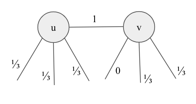
Figure 8: The decrease case in Lemma 3.3a, labelled with -values after the decrease is performed. If none of the edges in are decreased, then (conditioned on ) the analysis from the even case (3.2.1) gives
Now consider the case that an edge in is decreased. Let and let denote the set of two nonzero edges in (see Figure 8). Applying Theorem 2.9 and the fact that , we have . By Theorem 2.8,
We apply Theorem 2.9 again to lower bound by
Since the same calculation may be repeated with and (as ), we have
So comparing both cases, we have that conditioned on , if there is a local decrease then
- A local increase occurs.
We first note that the probability of no edge in being increased is at least , in which case the analysis from the even case (3.2.1) gives
Now consider the case that an edge , say in , is increased from to . Let . Since , by Markov’s inequality we have . Furthermore, by Theorem 2.8. In total, . Applying Theorem 2.8 thrice more, we obtain
which by Theorem 2.9 gives us
This yields, in the case that an edge in is increased,
Since the probability that no edge in is increased is at least , and , in the worst case we have that, conditioned on , if there is a local increase then
Now comparing the cases of local increase and decrease and removing the conditioning of , we obtain in the worst case
which is the bound we sought. ∎
Proof of Lemma 3.3b, Odd Case.
The MatInt claims. Fix a matching such that (w.p. ); each of have two other internal edges, each with -value . Call these four interesting edges. Suppose has two edges, then we perform a local increase step. Condition on the edge in chosen as part of the local increase: in the worst case it is incident to the endpoint of two of the interesting edges.
- •
Then w.p. it increases one of the interesting edges from to . The total -value of interesting edges becomes . By the same argument as for the even case, the tree contains exactly one interesting edge with probability at least .
- •
With the remaining probability , the increase is not to an interesting edge, and hence we succeed with the original probability .
The total probability of success is therefore .
On the other hand, if is empty, then we perform a local decrease step. Condition on the boundary edge chosen in the first part of the local decrease. In the worst case it is one of the boundary edges incident to either or . One of the interesting edges is reduced w.p. , from to . If that happens, the total -value of interesting edges sums to . The connectivity of the spanning tree means that every tree we sample with these marginals will have exactly one interesting edge.
Hence, in either case, we have exactly one of these four internal edges and satisfy the condition of the claim with probability , conditioned on having . The overall probability is therefore at least .
The MaxEnt claims. Observe that the edge will always contribute either: 0 to both the degree of in and the degree of in OR 1 to both the degree of in and the degree of in . Thus, to lower bound the probability that and have different parities in , we will not need to consider whether or not is in .
Let be the two internal edges in and be the two internal edges in . (We know each set has exactly two edges because are each boundary vertices.) Let be the two external edges incident to , respectively. We take cases based on (a) whether a local increase or decrease is performed, (b) whether or not any of are changed by the local increase or decrease, and (c) whether or not . Note that for (b), we do not take subcases on whether or not is changed, by the above paragraph. Also note that for (c), we consider whether in order to determine the marginals of prior to a local increase or decrease.
- Case I.N.1: local increase occurs, not touched, .
- Case I.N.2: local increase occurs, not touched, .
This case includes the two subcases and , which are cases 2 and 3 in the proof of Lemma 3.3b (see 3.2.1) and yield lower bounds on the desired probabilitiy of and , respectively. Finally, there is one more subcase for the case where is odd, namely, , since we may have . Since in this subcase are all -valued edges, we have the same bound from Case 1 of the even case in the proof of Lemma 3.3, namely, .
- Case I.T.1: local increase occurs, touched, .
One of the edges is increased from to , while the rest are still -valued, since . Hence, . Furthermore, note that we must have . This gives
- Case I.T.2: local increase occurs, touched, .
Just as in Case I.N.2., there are three subcases. First consider the subcase of . In this subcase, cannot be increased, so we know . By Theorem 2.9, .
Next, consider the subcase that only . Then, we have and hence by Theorem 2.9, .
For the final subcase that , we have and since , we have .
This concludes the local increase cases. We move on to the local decrease cases.
- Case D.N.1: local decrease occurs, not touched, .
This is the same case as I.N.1., giving a bound of .
- Case D.N.2: local decrease occurs, not touched, .
This is the same case as I.N.2., taking only the first subcase (), since in a local decrease. Thus the lower bound here is .
- Case D.T.1: local decrease occurs, touched, .
Since , we know start of as -valued. Then, w.l.o.g., say is decreased to 0. Then, But since , this gives
- Case D.T.2: local decrease occurs, touched, .
Since in a local decrease , we have w.l.o.g. that and that is not decreased. So Since we know , we instead study ; by Theorem 2.9, we have .
The minimum of all the boxed quantities is . Hence, for the odd case of Lemma 3.3b, we obtain the desired bound
Appendix C Charging Proof Details
Proof of Averaging Argument, §6.5.1, Case 4.
We will use an averaging argument to show that the expected charge is no worse than We construct a flow network as in the proof of Lemma 6.3 in order to show there exists a function satisfying constraint (7) for . Then we can apply a charging scheme like the one described in Case 1 using the function . The flow network is as follows: take the graph and add a source node and a sink node . Connect to every vertex in , and label with capacity or based on whether corresponds to a non- degree, degree, or cycle edge, respectively. To find satisfying the properties in the above paragraph, by Lemma 1 we need to show that for each ,
where and are the numbers of vertices in corresponding to non- degree, degree, and cycle edges, respectively. Note .
Lemma 6.4 showed that
Now taking a convex combination of the three inequalities above we obtain:
which is precisely what we sought to show. This concludes Case 4. ∎
Appendix D Symmetry Lemma
Claim D.1 (Symmetry Lemma).
For any graph with each edge having , let be a random set of edges faithful to the marginals, i.e., . For any two edges , let denote the probabilities of being respectively. Then and .
Proof.
Observe that . Moreover, . Hence, , proving the first statement. Now, giving , proving the second. ∎