∎
On the asymptotics of 3+1D cosmologies with bounded scalar potential and isometry group forming 2-dimensional orbits
Abstract
We study the onset of inflation in 3+1 dimensional cosmologies with an inflationary potential satisfying , matter satisfying the dominant and strong energy conditions, and with spatial slices that can be foliated by 2-dimensional surfaces that are orbits under an isometry group. Assuming an initial Cauchy slice with positive mean curvature everywhere, we show, via mean curvature flow, that there exists a family of spatial slices parameterized by , whose volume grows between the flat slicings in de Sitter spaces with cosmological constants and . In particular, inflationary expansion indeed occurs in this setting with inhomogeneous initial conditions. Finally, we apply this “inflationary time coordinate” to study asymptotics of the variation in the metric, the average stress-energy tensor, and the dynamics of an inflaton field on a spatial slice.
Keywords:
Inflation, non-homogeneous initial conditions, mean curvature flow.1 Introduction
Inflation has been a highly successful theory in resolving the horizon, flatness, and magnetic monopole problems in cosmology guth1981; Linde:1981mu; Albrecht:1982wi; Linde:1983gd. Furthermore, it has shown remarkable agreement with observational data from the Cosmic Microwave Background (see for example Aghanim:2018eyx; Akrami:2018odb; Akrami:2019izv) and the Large-Scale Structure of the universe (see for example DAmico:2019fhj; Ivanov:2019pdj; Colas:2019ret; Abbott:2017wau; Abbott:2018wzc). Despite these triumphs, the standard analysis of inflation suffers from an unrealistic assumption of homogeneous initial conditions. Concretely, one assumes an initial region of space, on the order of the Hubble length during inflation, that is homogeneously filled with the inflationary scalar field (inflaton) at the top of its potential. Such fine-tuned initial conditions seem improbable, for which this issue is dubbed the “initial patch problem” (see for example Ijjas:2015hcc). More fundamentally, spatial homogeneity is widely thought to be a consequence of inflation, and not its cause. Hence, whether inflation can begin under inhomogeneous initial conditions has been an important question under debate.
Recently, significant progress on both numerical and analytic fronts have been made in this direction. On the numerical side, East:2015ggf; Clough:2016ymm; Clough:2017efm have found that inflation always begins from a large set of inhomogeneous initial conditions, enabled by developments in numerical relativity that can handle singularities and horizons Pretorius:2005gq. These numerical experiments seem to go a long way in showing that inflation does not generically need an initial homogenous patch. On the analytic end, Kleban:2016sqm has attained partial results in the general case of a positive cosmological constant without extra symmetries, via a combination of Mean Curvature Flow techniques (see for example gerhardtbook) and the Thurston Geometrization Classification (see besse1987einstein Theorem 4.35 and thurston1997three; 10.2307/2152760), under the assumptions of matter satisfying the weak energy condition and all space-time singularities being of the so-called crushing kind. Concretely, Kleban:2016sqm showed that for almost all topologies of the spatial slices of a cosmology, the volume of these slices is increasing and that there is always an open neighborhood that expands at least as fast as the flat slicing of de Sitter space. This is suggestive that the volume will expand to infinity, matter will dilute away, and the universe will resemble de Sitter space in arbitrarily large regions of spacetime. These statements were proven in 2+1 dimensions (with the additional assumption that matter satisfies the strong and the dominant energy conditions in Creminelli:2019pdh and stronger assumptions on the matter content and initial conditions in Barrow:2006cw). In 3+1 dimensions, creminelli2020sitter proved these results plus the pointwise convergence of the metric to that of de Sitter space and ‘physical equivalence’ to de Sitter, under the additional assumption that there exists an isometry group forming 2-dimensional orbits on the spatial slices of the cosmology. In particular, the latter convergence is a concrete, affirmative instance of the de Sitter no-hair conjecture (see for example Gibbons:1977mu; Hawking:1981fz; Wald:1983ky; Kleban:2016sqm) which states that initially sufficiently expanding cosmologies should asymptote to de Sitter space in the presence of a positive cosmological constant.
Though the above analytic results are already suggestive that the onset of inflation doesn’t necessitate an initial homogeneous patch, all of them assumed a positive cosmological constant as a model of the underlying inflationary potential. In this paper, we focus on 3+1 dimensions with the isometry assumptions of creminelli2020sitter and an inflationary potential satisfying , which supersedes the previously-supposed cosmological constant (which can be seen as the limiting case ). We show that if , there is a family of spacelike hypersurfaces , parameterized by a flow time , that reaches arbitrarily late times (as defined by the Cauchy time function of the cosmology) and whose volumes grow between those de Sitter spaces with cosmological constants and in the flat slicing. In other words, inflationary expansion indeed occurs under our more general assumptions, with as a new time coordinate.
We also present partial results for the variation of the metric on , the dilution of matter, and the asymptotic dynamics of an inflaton. These bounds are suggestive (but do not prove) that the metric approaches a spatially homogeneous one on the slices for late enough . All-in-all, our results govern the asymptotics of a more realistic model of inflation.
2 Geometric Set-up
We require the general assumptions of Creminelli:2019pdh with the cosmological constant replaced by a potential and the symmetry assumptions of creminelli2020sitter. The former endows certain existence results that enable studying the cosmology via mean curvature flow (MCF) while the latter partially reduces the problem to the study of 2-dimensional manifolds whose Ricci scalar is intricately connected to its Euler characteristic.
2.1 General Assumptions
The general geometric assumptions are:
- (A)
(Initially expanding slice in cosmology) There is a “cosmology”, which is defined as a connected 3 + 1 dimensional spacetime with a compact Cauchy surface. This implies that the spacetime is topologically where is a compact 3-manifold, and that it can be foliated by a family of topologically identical Cauchy surfaces gerochdomain. We fix one such foliation, i.e. such a time function , with and being a non-zero timelike past-directed vector field, and with associated lapse function : , . We consider manifolds that are initially expanding everywhere. That is, there is an initial slice , where everywhere, with being the mean curvature with respect to the future pointing normal to . In particular, such a slice exists if one has a global crushing singularity in the past.
- (B)
(EFE) satisfies Einstein’s field equation
(1) where is the Ricci tensor, is the scalar curvature, and is the stress-energy tensor. Next, we also suppose can be decomposed as
(2) where is a potential satisfying for constants and is the reduced stress-energy tensor.
- (C)
(Energy conditions) so the potential is positive. The reduced stress-energy tensor satisfies the Dominant Energy Condition (DEC) and the Strong Energy Condition (SEC). The DEC states that is a future-directed timelike or null vector for any future-directed timelike vector . The DEC implies the Weak Energy Condition (WEC), for all time-like vectors . The SEC, in 3+1D, states for any future-directed timelike vector .
- (D)
(Crushing singularities) We presume that the only spacetime singularities are of the crushing kind given in Definition 1 (thus, those with zero spatial volume):
Definition 1.
(Definition 1 in Creminelli:2019pdh, c.f. Definitions 2.9 — 2.11 in eardleytime). A future crushing function is a globally defined function on such that on a globally hyperbolic neighborhood , is a Cauchy time function with range ( is a constant), and such that the level sets , with , have mean curvature .11 1 For example in a Schwarzschild-de Sitter spacetime in the standard coordinates, one could take to be a function of for close to 0, so the level sets would be . We shall say that a cosmology has potential singularities only of the crushing kind if there is an open set such that, the inverse of the lapse of the foliation is bounded outside , and such that contains a Cauchy slice and admits a future crushing function with respect to which is bounded in for any given .
Physically, corresponds to a subset of the interior of black holes and we are imposing the condition that all possible pathologies occur as .
Notably, our assumptions allow for an inflationary potential associated with the stress-energy tensor of an inflaton field plus the stress-energy tensor of residual matter , assuming also satisfies the DEC and SEC. Such a stress energy tensor takes the form:
| (3) |
Note that this more realistic inflationary stress-energy tensor is precluded by creminelli2020sitter which models the inflationary potential by a positive cosmological constant. We will work with a general before specializing to this particular one in analyzing the dynamics of the inflaton in Section 6.3.
Now, since is bounded on the compact initial surface , we pick large enough such that . Then, we can redefine a new time function on , which we call from now on, whose lapse is set to in the region .
2.2 Mean Curvature Flow
The general geometric assumptions above enable us to study via the Mean Curvature Flow (MCF) of co-dimension one spacelike surfaces in a Lorentzian manifold. This is defined as the deformation of a slice as follows: is, at each a mapping between the initial spatial manifold (parametrized by ) and the global spacetime, . The evolution under is given by (see for instance eckerhuisken):
| (4) |
where is the future-oriented vector orthonormal to the surface of constant . We denote by the geometric image of and the mean curvature at with respect to the future pointing normal to . MCF in Lorentzian manifolds is endowed with many regularity properties, which are rare in the context of Riemannian manifolds. Importantly, the flow is globally graphical and the spatial volume of is non-decreasing . In our case, two additional properties are: a) remains spacelike; in fact the volume form of is non-decreasing but it would vanish anywhere where becomes null and, b) everywhere is preserved on (see e.g. gerhardtbook, Proposition 2.7.1).
Our assumptions, restricted to the case where the potential is just a positive cosmological constant , were used in Creminelli:2019pdh to prove the useful statements about the maximum of and the existence of the MCF for all . As pointed out in pg. 11 of Creminelli:2019pdh, modifications of their results lead to essentially the same consequences in the current situation.
Theorem 2.1
(Bound on the Maximum of ). Creminelli:2019pdh Let be hypersurfaces satisfying the MCF equation, in an interval , inside the smooth dimensional Lorentzian manifold satisfying Eq. (1) with for some and fulfilling the SEC. Then, defining , we have for ,
| (5) |
with and . So the maximum of , if larger than decays exponentially fast towards with a rate given .
Applying the above to and which satisfies22 2 Indeed, for any future-directed timelike vector , since satisfies the SEC, , and since is timelike. the SEC, we obtain for values of , at which the flow exists for all ,
| (6) |
where . For convenience, we also rewrite the above as
| (7) |
where .
Now, this upper bound on the maximum of then implies an upper bound on the height function defined by (i.e. is the Cauchy time function restricted to ) and the avoidance of crushing singularities.
Theorem 2.2
(Height bound). Creminelli:2019pdh Let with given in Definition 1 and . There exists a constant (depending on and
) such that the following holds.
Provided that is in for all , we have
for all and .
Theorem 2.3
(Avoidance of crushing singularities). Creminelli:2019pdh If the initial surface of the flow has then stays away from crushing singularity. More precisely, for any such that is in , the flow remains in .
Theorem 2.3 implies that the flow remains smooth while Theorem 2.2 implies that stays in a compact region for . Combined with the short-term existence result below, they imply that the MCF exists for all and .
Theorem 2.4
(Short-term existence of MCF). ecker_1993 Let be a smooth -dimensional Lorentzian manifold satisfying Eq. (1) with for some and satisfying the WEC. Let be a compact smooth spacelike hypersurface in . Then there exists a unique family of smooth compact spacelike hypersurfaces satisfying the MCF equation (4), in an interval for some and having initial data . Moreover, if this family stays inside a smooth compact region of then the solution can be extended beyond .
Note that Theorem 2.4 is indeed applicable with and which satisfies33 3 For any future-directed timelike vector , let be causal and future-directed since satisfies the DEC. Now, define which is future-directed as where since are future directed, , and since is timelike. Next, is also causal since where since is causal and also, , and as before. the DEC and hence the WEC.
Finally, applying Theorem 2.3 with implies always stays in such that for purposes of MCF, the lapse can be treated as unity. Ultimately, the global existence result of this section enables us to study via MCF while the upper bound in Eq. (6) will grant us control over geometric quantities.
2.3 Symmetry Assumptions
We also assume that either of the symmetry assumptions of creminelli2020sitter holds. These enable the control of geometric quantities by topological properties of orbit surfaces.
- (A)
(Simplified symmetry assumption) There is a Lie group which acts on such that the induced action on is by isometries, and such that the orbits under are closed surfaces. Assume that the orbits of are two-sided (i.e, with trivial normal bundle).
- (B)
(General symmetry assumption). There is a Lie group which acts on some cover such that the induced action on is by isometries. Assume further that the orbits under are two dimensional complete (i.e. with no edges) surfaces, and that for each such orbit its projection is a two-sided surface.
Notably, the induced actions of in Assumption A and in Assumption B on both map and thus its flow to themselves, thus preserving level sets of . Furthermore, if is an orbit under in Assumption A or the projection of an orbit under in Assumption B, all intrinsic and extrinsic scalar quantities on (such as in Section 3) are constant along it.
An example of allowed by our assumptions is sketched in Fig. 1. We defer more concrete constructions to Section 3 of creminelli2020sitter.

Our symmetry assumptions also enable the following decomposition of the induced metric on for a fixed creminelli2020sitter. Consider the foliation of by the orbits of (or more generally, by the projections of the orbits of ). By our two-sidedness assumption, there exists a global unit normal vector to this foliation. Let be the parameter along the flow lines of , which is thus a signed distance function. Due to the isometries of (or ), the metric on has the warped product form
| (8) |
where is a two-dimensional metric of constant curvature.
By passing to a double cover, we can assume without loss of generality that the orbit surfaces are orientable. Thus, each such orbit is a two-dimensional orientable surface, with Euler characteristic . Later, this will be used to control the Ricci scalar on these orbits via the Gauss-Bonnet theorem.
3 Notation and statement of main results
3.1 Notation
We will follow the notation in creminelli2020sitter. The Riemann tensor is defined by , the Ricci tensor by (we also use the notation , with being two vectors), the Ricci scalar (also known as scalar curvature) by .
A time slice has an induced Riemannian metric , and we can write , where is the spacetime metric (we use the mostly-plus convention) and is orthonormal to , , and future-directed. The extrinsic curvature (also known as second fundamental form) of these slices is defined as , satisfying and with trace (also known as mean curvature) , and traceless part (with our sign convention corresponds to expansion). We also define where since is a tensor projected on the spatial hypersurfaces. The Ricci tensor and Ricci scalar (scalar curvature) associated with the induced metric on the -dimensional slices are denoted, respectively, by and .
Similarly, each 2-dimensional symmetric orbit (or covering image of a symmetric orbit) within has induced metric satisfying , where is orthogonal to and to , and . The extrinsic curvature (second fundamental form) of this slice within is defined as , satisfying and with trace (mean curvature) . The Ricci tensor and Ricci scalar (scalar curvature) associated with the induced metric on a -dimensional slices are denoted by and respectively.
We denote by the capital letters with , non-negative constants that depend only on the intrinsic and extrinsic properties of the initial 3-manifold of the flow: . We refer to such constants as universal.
3.2 Main Results
We summarize the main result of our paper as follows:
Theorem 3.1
Let be a spacetime satisfying assumptions of Section 2.1, in addition to the symmetry assumptions of Section 2.3. If the orbit surfaces are spheres, one needs to further assume that the minimal area of an orbit surface in satisfies
| (9) |
where depends only on , , . If , for every , there exists some such that for ,
- (A)
(Volume grows between de Sitter spaces in the flat slicing with cosmological constants and ) Letting denote the volume of ,
(10) - (B)
(Majority of the physical volume reaches arbitrarily late times). Let be the height function defined by . In other words, . Without loss of generality, also suppose . For any , denoting as the physical volume of the subset of with , we have
(11) Combined with the lower bound in (A), this implies for all ,
(12) such that the majority of physical volume has height growing at least linearly in . We remark here that due to Eq. (6), so the height function also grows at most linearly in .
Theorem 3.1(A) shows that there exists a family of spacelike surfaces with volume exponentially expanding between those of flat slicings of de Sitter spaces with cosmological constants and . In particular, inflationary expansion occurs in the absence of homogeneous initial conditions in this case, though an everywhere positive mean curvature on the initial slice is still assumed .
Next, the exponentially expanding volume of renders as an ideal “MCF coordinate chart” for modelling cosmological inflation. To this end, Theorem 3.1(B) shows that this coordinate patch indeed covers a large subset of the cosmology and is hence useful as a physical description of the future.
The proof of Theorem 3.1 (and more) occupies the upcoming two sections. In Section 4 we study the asymptotic behavior of the minimal area of orbit surfaces, length of the transverse geodesics on , and the volume of (Theorem 3.1(A) ). Theorem 3.1(B) and the asymptotics of the average height on are covered in Section 5. Finally, Section 6 discusses several applications of the MCF coordinate chart concerning the variation of metric in the z-direction, the dilution of the reduced stress-energy tensor, the asymptotic evolution of an inflaton as well as directions for future work.
4 Asymptotic Geometric Bounds
In this section, we follow the approach of creminelli2020sitter to derive asymptotic bounds for various geometric quantities. The main idea is to repeatedly reduce the dimension of the problem until a two-dimensional orbit surface , whose can be upper bounded in terms its Euler characteristic . To this end, the Gauss equation will be essential in relating the Ricci tensor of a submanifold to that of its parent manifold. Applying the traced Gauss equation to within , we obtain (see for instance Wald:1984rg, Eq.
| (13) |
Now, substituting into Eq. (1) yields
| (14) |
such that Eq. (13) becomes
| (15) |
where
| (16) |
In coordinate form:
| (17) |
where since by the WEC and using ,
| (18) |
Meanwhile, the traced Gauss equations for a surface orbit within (see creminelli2020sitter Eq. (39)) imply
| (19) |
In reducing the problem to lower dimensions, Eqns. (17) and (19) relate Ricci scalars on and as well as between and respectively.
4.1 Orbit surfaces
The main objective of this section is an upper bound for on any orbit surface . Denote as the area of a two-dimensional orbit at coordinate , defined in Eq. (8), and as the minimal surface area of an orbit on . From the Gauss-Bonnet formula, which implies
| (20) |
where . Now, we show that if , grows between the two-dimensional spatial slices of de Sitter spaces in the flat slicing with cosmological constants , up to a correction that approaches zero as (44 4 The time evolution of topological surfaces in a similar setup was also studied in Mirbabayi:2018suw.). This exponential growth of will imply that the upper bound for in Eq. (20) decays exponentially if is positive.
To prove the above claim, we will consider a differential equation for . This is facilitated by the below standard lemma which shows that a minimizer has a well-defined derivative almost everywhere and obeys the fundamental theorem of calculus.
Lemma 1
(Hamilton’s trick (c.f mantegazza Lemma 2.1.3)). Let be a smooth function with being compact, and set to be the minimizer of on :
| (21) |
Then is a Lipschitz function, and thus, differentiable almost everywhere and obeying the fundamental theorem of calculus. Moreover, if is a point of differentiability of , and if is such that then
| (22) |
Next, we derive a few useful lemmas for our estimates. Lemma 2 enables us to wrap up various bounds once we have shown the logarithmic derivative of a quantity is a constant up to an exponentially decaying correction.
Lemma 2
Let be a non-negative function that is differentiable almost everywhere and satisfies the fundamental theorem of calculus. Furthermore, suppose that at points of differentiability, there are constants with such that
| (23) |
where . Then for every , there exists large enough such that for any ,
| (24) |
Similarly, if
| (25) |
where , then for every , there exists large enough such that for any ,
| (26) |
Proof.
We only prove the upper bound as the proof works almost verbatim for the lower bound. Since , for any , there exists large enough such that . Thus, integrating both sides of Eq. (23) from to ,
| (27) |
Upon exponentiation, we obtain Eq. (24).
∎
The next two technical lemmas are necessary due to the looseness in the range of the inflationary potential .
Lemma 3
Let for . The optimization problem
subject to the constraints (with being some constants with )
has the solution with .
Proof.
Firstly, observe that the first constraint implies . Now, we argue that the minimizer of must occur on the curve . Otherwise so would result in a smaller value of since is decreasing in .
Next, we show that there is no local minimum of in the interior of . Otherwise, let and suppose the minimizer is an interior point. By the method of Lagrange multipliers, we must have or
| (28) |
which is a contradiction since (). Hence, the minimizer must occur at which are the points and , at which takes respective values and . Some algebra then shows for so the minimizer is . ∎
For a slightly technical reason, we need to modify Lemma 3 as follows.
Lemma 4
Suppose with and satisfy the new constraints,
where , and . Then,
| (29) |
| (30) |
where
| (31) |
| (32) |
| (33) |
| (34) |
are non-negative increasing functions with as while and as .
Proof.
Firstly, we consider the following auxiliary problem. Let with and suppose (with , being some constants and )
Then, we claim that
| (35) |
| (36) |
To prove these, observe that is individually increasing in both under the constraints. Hence, the maximum of occurs at .
| (37) |
where we have used the inequality for .
Equipped with these lemmas, we obtain the following bounds for .
Theorem 4.1
Denote by the minimal area of a surface orbit and its Euler characteristic. Suppose . Then, for every , if either or, if and also where as in Eq. (6), there exists such that for all .
| (40) |
where
| (41) |
Remark 1.
The condition ensures that . Technically, Eq. (40) holds for even without this condition, though the lower bound will not be as meaningful.
Proof.
Firstly, we show that on a minimal surface orbit, . By the Riccatti equation (primes indicate derivative with respect to ),
| (42) |
Now, substituting Eq. (42) into Eq. (19) to eliminate , we obtain
| (43) |
Recall that by the first variation of area formula, where is the volume element of the surface orbit. Hence, on the minimal -slice, and such that Eq. (43) implies
| (44) |
Substituting this into Eq. (18) and applying Eq. (20), yields on a minimal slice,
| (45) |
Next, we obtain a differential equation for the evolution of . The evolution of the metric under MCF is given by (see eckerhuisken, Proposition 3.1)
| (46) |
Also, note that in general, if are local coordinates around a point on a orbit surface at flow time (not necessarily of minimal area), we have
| (47) |
where the indices only run over (corresponding to the tangent vectors and ). This will be used in the relationship (where is the area of any orbit)
| (48) |
which is applicable even to by Hamilton’s trick (Lemma 1). Hence, we are left with bounding the integrand on the R.H.S of Eq. (48) on a minimal -slice. For any point on the -slice, we can without loss of generality assume that are local orthonormal coordinates such that by the triangle and Cauchy-Schwartz inequalities. Thus,
| (49) |
such that multiplying the above by and applying Lemma 4 to , , and , with in light of Eq. (45), due to Eq. (6),
| (50) |
where is decreasing in and , with and defined as in Lemma 4. Combining this with Eq. (48) and Lemma 1,
| (51) |
If such that and , Lemma 2 immediately implies the lower bound of Eq. (40) since . Otherwise if , there exists large enough such that for . Since is an increasing function and as , there exists a large enough such that as long as , so
| (52) |
where (recall is decreasing). As a result, we get that if with
| (53) |
then on . Furthermore, we see that for all such that ,
| ( and our choice of ) | ||||
| (54) |
which shows that if on with , we also have on some extended interval for some . To see this, observe that the R.H.S of Eq. (51) is at as in Eq. (54). The continuity of (since it is Lipschitz by Lemma 1) and of the R.H.S of Eq. (51) in and in then implies that there exists some such that for points of differentiability in such that for any , .
Thus, letting , we must have otherwise by continuity such that the extension property above implies that on , violating the supremum property of . Hence, for all such that Eq. (54) holds for all .
Then, we have the non-optimal estimate upon integrating Eq. (54) such that . Recalling , both and terms in Eq. (51) are exponentially decaying in so Lemma 2 implies the lower bound of Eq. (40) for if .
Similarly, from the upper bound of Lemma 4 (with the same substitutions for as before),
| (55) |
where and . Combining this with Eq. (48) and Lemma 1,
| (56) |
Now if so , Lemma 2 immediately implies the upper bound of Eq. (40) since . Otherwise if and , the lower bound of Eq. (40) shows . Hence, Lemma 2 again implies the upper bound of Eq. (40). ∎
Notice that the additional requirement in the case of the sphere depends exponentially on the initial conditions (see Eq. (53)). This is different from what happens in the case of complete homogeneity where, for Bianchi-IX universes, one has to impose a lower bound on Wald:1983ky. This bound however does not depend exponentially on the initial conditions.
Henceforth, we choose in Theorem 4.1 for a fixed .
Corollary 1
Suppose the conditions of Theorem 4.1 hold. Substituting the lower bound of Eq. (40) into Eq. (20), we have for ,
| (57) |
4.2 Transverse Length and Volume
In this section, we derive bounds for the asymptotic growth of the volume and “tranverse” length of where the latter is defined as follows. By the form of the metric in Eq. (8), it is straightforward to check that if a geodesic is at a point tangent to the vector (unit normal to the foliation of by orbit surfaces), it is tangent to everywhere. Denote therefore by the length, at time , of any geodesic that is parallel to the -direction, from an initial orbit surface to itself.
Firstly, we derive a lemma for the asymptotic bounds of averages of . This is important as the mean curvature controls the growth of various geometric quantities under MCF.
Below, denotes the volume form on . Furthermore, for any smooth function , we denote and .
Lemma 5
We have
| (58) |
Furthermore, under the conditions of Theorem 4.1, for ,
| (59) |
In particular, since ,
| (60) |
Proof.
The upper bounds are consequences of the pointwise bound in Eq. (7). For the lower bound, integrating Eq. (43) from to and noting that since the endpoints refer to the same -coordinate, we obtain
| (61) |
Integrating Eq. (18) from to and applying the above inequality,
| (62) |
Hence, by Eq. (57), we obtain upon dividing by ,
| (63) |
The same proof works for , by replacing integrals above by integrals over . ∎
The next theorem describes the asymptotic growth of and . In particular, and grow between what are expected of de Sitter spaces in the flat slicing with cosmological constants , with the latter having a correction term that approaches zero as .
Theorem 4.2
Remark 2.
If , then so Eq. (65) implies grows exponentially.
Proof.
From such that , we obtain for ,
| (66) |
due to Lemma 5. Applying Lemma 2, we obtain Eq. (64). Next, we compute
| (67) |
By the triangle and Cauchy-Schwartz inequalities,
| (68) |
Expressing the two equations above in terms of averages along the -direction, we have
| (69) |
| (70) |
which imply
| (71) |
Furthermore from Lemma 5, we have for (where we have used the inequality in the second equation below)
| (72) |
| (73) |
which correspond to the first two constraints in Lemma 4 with , , , , , , , . In light of Eq. (71), using in Lemma 4 ,
| (74) |
4.3 Flow Reset
For a fixed in Theorem 4.2, let where the latter condition is such that by Eq. (6). Now, for the ease of notation, let us re-define the initial time of the flow as to be , so from now on . Note that estimates (6) and (7) still hold (in fact, with and ).
In particular, we have, for every ,
| (75) |
| (76) |
| (77) |
| (78) |
| (79) |
| (80) |
where .
5 MCF Probes Large Regions of Cosmology
The exponentially expanding volume of renders an ideal time coordinate for modelling inflation (when combined with the spatial coordinate on ). However, can only be a meaningful coordinate if the slices probe a large subset of the cosmology. Physically, the main possible pathology is the flow slowing down to a halt, as it encounter black holes in the cosmology (such that approaches zero), in an effort to avoid them. This is not a defect of MCF per say but, by design, a mechanism that enables us to study smooth regions of the cosmology (expected to dominate on the large-scale), without having to explicitly handle singularities. That said, we do have to check that the flow does not trivially stop everywhere and is able to reach large regions of the cosmology.
In the context of a positive cosmological constant , creminelli2020sitter achieved this by proving that is in fact a foliation of the future . Inadvertently, this implies that the cosmology does not have any crushing singularities and is thus geodesically complete (since the only spacetime singularities are assumed to be of the crushing kind). Their result thus precludes black holes expected to be physically relevant.
For a more general inflationary potential , we hereby prove weaker statements which show that probes a large subset of the future. Concretely, we show that almost all of the total physical volume on has height that approaches as and, in fact the heights of these points grow at least as fast as . Though we do not know if black holes indeed form, our results do not explicitly preclude black holes in the cosmology.
Below, we assume without loss of generality that (otherwise one can redefine such a by subtracting a constant). Furthermore, we use the notation for any subset .
Theorem 5.1
For any and ,
| (81) |
As a result, for every ,
| (82) |
which shows that almost all of the physical volume of has height growing at least as fast as asymptotically.
Proof.
Firstly, observe that
| (83) |
where we have applied the reverse Cauchy-Schwartz inequality for timelike vectors in the second step (note that since is past-directed while is future-directed). Hence, for such that , Eq. (83) implies
| (84) |
such that since for , we have
| (85) |
and from the evolution equation ,
| (86) |
at these points. Then,
| (87) |
Substituting and recalling that in light of the lower bound in Eq. (64),
| (88) |
Finally, since is arbitrary, we obtain Eq. (82). ∎
We also have the following bounds on the max and average heights and on .
Corollary 2
| (89) |
Proof.
The only non-trivial inequalities are the left-most and the right-most ones. For the former, since is increasing in due to Eq. (83), for any and . Notably, for any and ,
| (90) |
Taking and applying Eq. (82) yields for all ,
| (91) |
Finally, taking gives the left-most inequality. For the right-most inequality, Lemma 1 implies
| (92) |
where and in the second expression are parallel at the maximizer of (so ). Integrating Eq. (92) yields after which taking yields the right-most inequality. ∎
6 Auxiliary Results
Having established that is a useful time coordinate which asymptotically describes the future of the cosmology, we explore a few ramifications of using such a coordinate system.
6.1 Variation of Metric in -direction
Observe that a priori, there might be large regions where and respectively. In these regions, the de Sitter no-hair theorem in creminelli2020sitter suggests (but does not prove) that the metrics in these cases approach those of de Sitter with cosmological constants and respectively. Then, the spatial metric of could vary significantly across these regions as grows. In this section, for large , we show that varies much more weakly along the -direction than the extreme case described. In particular, our results suggest that such hypothetical de Sitter domains (if they exist) must be separated by a physical distance that tends to infinity as , illustrating that a physical observer cannot experience two different cosmological constants at late enough times.
The propagation of the metric along the level sets is given by the second fundamental form (extrinsic curvature):
| (93) |
so we proceed by controlling . Firstly, Eq. (18) implies the following pointwise bound on ,
| (94) |
where we have applied Eq. (7) in the second step. Substituting the pointwise bounds for and given by Eqs. (79) and (94) into Eq. (43),
| (95) |
Using by the Cauchy-Schwartz inequality and noting that and the maximum and minimum of , we obtain the following pointwise bound
| (96) |
Integrating Section 6.1 along the z-direction and using the pointwise bound Section 6.1,
| (97) |
Using the Cauchy-Schwartz equality and the inequality ,
| (98) |
Equipped with this bound, we proceed with bounding the variation in the metric. For any product coordinate system on of the form where is as before and are tangent to each surface orbit, Eq. (93) implies
| (99) |
Integrating this from to and using Eq. (98), with ,
| (100) |
One consequence of the above is as follows. Suppose there are two points such that under MCF, at these points expand as in de Sitter with different cosmological constants in the FLRW slicing with . Now, let denote the respective -coordinates of on (identified via MCF). Then since and ,
which implies by Eq. (100). Notably, as , showing that these points must have a diverging physical separation in .
6.2 Dilution of Reduced Stress-Energy Tensor
Next, we show that as a consequence of inflationary expansion, matter partially dilutes and the reduced stress-energy tensor is at most almost everywhere. We achieve this by bounding the average of (by the WEC) on a transverse geodesic. Note that
| (Eq. (17)) | ||||
| (Eq. (61)) | ||||
| (101) |
where we have applied Eqns. (79) and (7) in the last inequality. Because of the DEC, is at least as large as the absolute value of any other component of the stress tensor in an orthonormal frame where is the timelike vector55 5 This is actually an equivalent definition of the DEC Hawking:1973uf as it is straightforward to verify.. We therefore define a vierbein , such that , with being the Minkowski metric. We choose . By the DEC, we have
| (102) | ||||
| (103) |
Since, by the symmetries of the problem, is uniform on the slices at constant , we see that in almost-all of the ever-growing -direction, has to be at most on the order of up to a correction of order on a z-distance that is at most an fraction of the total length . Physically, this suggests that for small enough , the influences of matter and the inflaton kinetic energy are bounded and the potential component is the dominant factor in determining the asymptotic geometry.
6.3 Asymptotic Average Rolling of Scalar Field in Monotonic Potential
In this section, we devote our attention to the stress-energy tensor of an inflaton given by Eq. (3). Under the additional assumption that the potential is increasing (i.e. ), we show that asymptotically, the average rolling of in MCF coordinates resembles that of a slow-rolling solution in an expanding FLRW universe. Given a point , the metric of at is given by
| (104) |
This motivates our definition of the average rolling of on as . Now, the dynamics of is governed by the Klein-Gordon equation:
| (105) |
where the Laplace-Beltrami operator on is defined by
| (106) |
Here, we recall that is the spatial metric on . Below, we will adopt the additional assumption that (i.e. the potential is increasing). An example potential is depicted in Fig. 2.
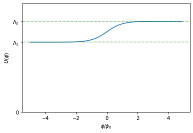
Theorem 6.1
Let evolve via the Klein-Gordon equation (105) with . Furthermore, suppose the conditions of Theorem 4.1 hold. Then,
| (107) |
| (108) |
In particular, if is bounded, we have
| (109) |
Proof.
Substituting Eq. (106) in Eq. (105), we obtain upon multiplying by and integrating over :
| (110) |
where in the second step, we have used Stokes’ theorem along with the fact that has no boundary to conclude that the spatial derivatives vanish upon integration. Next, we compute
| (111) |
where we have applied Section 6.3 and the equation in the second step. Now since , by a standard ODE argument, if for some , for all .
Concretely, suppose otherwise that for some . Then, define such that by continuity, . Then, Eq. (6.3) implies that . Then, the continuity of the R.H.S of Eq. (6.3) in implies that there exists such that on such that for , . However, this contradicts the infimum property of since there does not exist arbitrarily close to such that . Thus, for all .
In this case, we automatically have . Next, by Eqs. (75) and (80), we have the lower bound
| (112) |
Now, observe that since would result in the contradiction for large enough . Thus, taking the of Section 6.3 yields
| (113) |
The only other possible case is for all , for which we immediately have . Now, for large enough , the R.H.S. of Eq. (80) is larger than . Then, Section 6.3 becomes for large enough
| (114) |
or in other words,
| (115) |
which shows that . In this second case, we actually have . ∎
Remark 3.
Consider the standard slow-roll model with a FLRW metric
| (116) |
where is a spatial metric, independent of , on a three-manifold of uniform curvature—that is, the space is either elliptical (closed), euclidean (flat), or hyperbolic (open). Under the traditional slow-roll assumptions at late enough times and assuming as , we have while . Meanwhile, since , we can rewrite Theorem 6.1 as and . Hence, the asymptotic bounds in Theorem 6.1 are reminiscent of a slow-roll inflaton in an expanding FLRW universe, up to an additional factor of .
7 Conclusion and Future Work
In summary, we have considered 3+1 dimensional cosmologies satisfying the Einstein equations with an inflationary potential satisfying with and matter satisfying the dominant and the strong energy conditions. In particular, our results allow for a non-flat inflaton potential as opposed to only a cosmological constant assumed by previous work.
We have assumed that the only potential singularities are of the crushing kind, and that the spatial slices are foliated by homogeneous but potentially anisotropic 2-surfaces. Though we assumed that the initial spatial slice has positive mean curvature everywhere, we do not require homogeneous initial conditions on .
By probing the geometry with mean curvature flow, we show that the family of mean curvature flow surfaces has physical volume expanding in , at exponential rates between those of flat slicings of de Sitter spaces with cosmological constants and . In particular, this result shows that inflationary expansion can indeed occur without homogeneous initial conditions and partially resolves the “initial patch problem”.
Future Directions: In the limiting case of a positive cosmological constant, creminelli2020sitter proved a de Sitter no-hair theorem where the metric converges pointwise to that of de Sitter space and the asymptotic geometry becomes physically indistinguishable from de Sitter space. Though our current bounds are too weak (in particular, the lower bound in Eq. (60) involves the average rather than the pointwise ), our partial results in Section 6 are highly suggestive that in the particular case of a dynamical inflaton with the stress-energy tensor in Eq. (3), a similar convergence to de Sitter space may occur, given a more refined analysis of the inflaton dynamics or slightly stronger assumptions on the cosmology. Concretely, Sections 6.1 and 6.2 show that the influence of the inflaton on the inhomogeneity of the geometry is bounded on ever-expanding regions. At the same time, Section 6.3 shows that, in some averaged sense, the inflaton is asymptotically rolling down the potential (or at least not rolling upward) so at late enough times, one expects the inflaton to converge to a constant . Then, we might be able to recover a de Sitter no-hair theorem for a cosmological constant .
Acknowledgments
We thank Paolo Creminelli for initial extensive collaboration in this project. We also thank Or Hershkovits and Andras Vasy for discussions.
References
- (1) A. H. Guth, Inflationary universe: A possible solution to the horizon and flatness problems, Phys. Rev. D 23 (Jan, 1981) 347–356.
- (2) A. D. Linde, A New Inflationary Universe Scenario: A Possible Solution of the Horizon, Flatness, Homogeneity, Isotropy and Primordial Monopole Problems, Adv. Ser. Astrophys. Cosmol. 3 (1987) 149–153.
- (3) A. Albrecht and P. J. Steinhardt, Cosmology for Grand Unified Theories with Radiatively Induced Symmetry Breaking, Adv. Ser. Astrophys. Cosmol. 3 (1987) 158–161.
- (4) A. D. Linde, Chaotic Inflation, Phys. Lett. B 129 (1983) 177–181.
- (5) Planck collaboration, N. Aghanim et al., Planck 2018 results. VI. Cosmological parameters, 1807.06209.
- (6) Planck collaboration, Y. Akrami et al., Planck 2018 results. X. Constraints on inflation, 1807.06211.
- (7) Planck collaboration, Y. Akrami et al., Planck 2018 results. IX. Constraints on primordial non-Gaussianity, 1905.05697.
- (8) The Cosmological Analysis of the SDSS/BOSS data from the Effective Field Theory of Large-Scale Structure, 1909.05271.
- (9) M. M. Ivanov, M. Simonović and M. Zaldarriaga, Cosmological Parameters from the BOSS Galaxy Power Spectrum, 1909.05277.
- (10) T. Colas, G. D’amico, L. Senatore, P. Zhang and F. Beutler, Efficient Cosmological Analysis of the SDSS/BOSS data from the Effective Field Theory of Large-Scale Structure, 1909.07951.
- (11) DES collaboration, T. M. C. Abbott et al., Dark Energy Survey year 1 results: Cosmological constraints from galaxy clustering and weak lensing, Phys. Rev. D98 (2018) 043526, [1708.01530].
- (12) DES collaboration, T. M. C. Abbott et al., Cosmological Constraints from Multiple Probes in the Dark Energy Survey, Phys. Rev. Lett. 122 (2019) 171301, [1811.02375].
- (13) A. Ijjas and P. J. Steinhardt, Implications of Planck2015 for inflationary, ekpyrotic and anamorphic bouncing cosmologies, Class. Quant. Grav. 33 (2016) 044001, [1512.09010].
- (14) W. E. East, M. Kleban, A. Linde and L. Senatore, Beginning inflation in an inhomogeneous universe, JCAP 1609 (2016) 010, [1511.05143].
- (15) K. Clough, E. A. Lim, B. S. DiNunno, W. Fischler, R. Flauger and S. Paban, Robustness of Inflation to Inhomogeneous Initial Conditions, JCAP 1709 (2017) 025, [1608.04408].
- (16) K. Clough, R. Flauger and E. A. Lim, Robustness of Inflation to Large Tensor Perturbations, JCAP 1805 (2018) 065, [1712.07352].
- (17) F. Pretorius, Evolution of binary black hole spacetimes, Phys. Rev. Lett. 95 (2005) 121101, [gr-qc/0507014].
- (18) M. Kleban and L. Senatore, Inhomogeneous Anisotropic Cosmology, JCAP 1610 (2016) 022, [1602.03520].
- (19) C. Gerhardt, Curvature Problems. International Press, Boston, 2006.
- (20) A. Besse, Einstein Manifolds. Classics in mathematics. World Publishing Company, 1987.
- (21) W. Thurston and S. Levy, Three-dimensional Geometry and Topology. No. v. 1 in Luis A.Caffarelli. Princeton University Press, 1997.
- (22) G. Perelman, Manifolds of positive ricci curvature with almost maximal volume, Journal of the American Mathematical Society 7 (1994) 299–305.
- (23) P. Creminelli, L. Senatore and A. Vasy, Asymptotic Behavior of Cosmologies with in 2+1 Dimensions, Commun. Math. Phys. 376 (2020) 1155–1170, [1902.00519].
- (24) J. D. Barrow, D. J. Shaw and C. G. Tsagas, Cosmology in three dimensions: Steps towards the general solution, Class. Quant. Grav. 23 (2006) 5291–5322, [gr-qc/0606025].
- (25) P. Creminelli, O. Hershkovits, L. Senatore and A. Vasy, A de sitter no-hair theorem for 3+1d cosmologies with isometry group forming 2-dimensional orbits, 2020.
- (26) G. Gibbons and S. Hawking, Cosmological Event Horizons, Thermodynamics, and Particle Creation, Phys. Rev. D 15 (1977) 2738–2751.
- (27) S. Hawking and I. Moss, Supercooled Phase Transitions in the Very Early Universe, Adv. Ser. Astrophys. Cosmol. 3 (1987) 154–157.
- (28) R. M. Wald, Asymptotic behavior of homogeneous cosmological models in the presence of a positive cosmological constant, Phys. Rev. D28 (1983) 2118–2120.
- (29) R. Geroch, Domain of dependence, Journal of Mathematical Physics 11 (1970) 437–449, [https://doi.org/10.1063/1.1665157].
- (30) D. M. Eardley and L. Smarr, Time functions in numerical relativity: Marginally bound dust collapse, Phys. Rev. D 19 (Apr, 1979) 2239–2259.
- (31) K. Ecker and G. Huisken, Parabolic methods for the construction of spacelike slices of prescribed mean curvature in cosmological spacetimes, Comm. Math. Phys. 135 (1991) 595–613.
- (32) M. Kleban and L. Senatore, Inhomogeneous anisotropic cosmology, Journal of Cosmology and Astroparticle Physics 2016 (02, 2016) .
- (33) K. Ecker, On mean curvature flow of spacelike hypersurfaces in asymptotically flat spacetimes, Journal of the Australian Mathematical Society. Series A. Pure Mathematics and Statistics 55 (1993) 41–59.
- (34) R. M. Wald, General Relativity. Chicago Univ. Pr., Chicago, USA, 1984, 10.7208/chicago/9780226870373.001.0001.
- (35) M. Mirbabayi, Topology of Cosmological Black Holes, JCAP 05 (2020) 029, [1810.01431].
- (36) C. Mantegazza, Lecture notes on mean curvature flow. Springer Basel AG, 2011.
- (37) S. Hawking and G. Ellis, The Large Scale Structure of Space-Time. Cambridge Monographs on Mathematical Physics. Cambridge University Press, 2, 2011, 10.1017/CBO9780511524646.