Dust continuum, CO and [Ci] 1-0 lines: Self-consistent mass estimates and the possibility of globally CO-‘dark’ galaxies at z=0.352020Dust continuum, CO and [Ci] 1-0 lines: Self-consistent mass estimates and the possibility of globally CO-‘dark’ galaxies at z=0.35–23
Abstract
We present ALMA observations of a small but statistically complete sample of twelve 250m selected galaxies at designed to measure their dust submillimeter continuum emission as well as their and atomic carbon [Ci](3P1-3P0) spectral lines. This is the first sample of galaxies with global measures of all three -mass tracers and which show star formation rates (4–26 yr) and infra-red luminosities () typical of star forming galaxies in their era. We find a surprising diversity of morphology and kinematic structure; one-third of the sample have evidence for interaction with nearby smaller galaxies, several sources have disjoint dust and gas morphology. Moreover two galaxies have very high / ratios for their global molecular gas reservoirs; if confirmed, such extreme intensity ratios in a sample of dust selected, massive star forming galaxies presents a challenge to our understanding of ISM. Finally, we use the emission of the three molecular gas tracers, to determine the carbon abundance, , and CO– conversion in our sample, using a weak prior that the gas-to-dust ratio is similar to that of the Milky Way for these massive and metal rich galaxies. Using a likelihood method which simultaneously uses all three gas tracer measurements, we find mean values and errors on the mean of and (or ) and (or ), where our starting assumption is that these metal rich galaxies have an average gas-to-dust ratio similar to that of the Milky Way centered on .
Keywords:
Galaxies: Local, Infrared, Star-forming, ISM1 Introduction
The cold neutral gas (i.e. Cold Neutral Medium (CNM) Hi and H2 gas) in galaxies is the main fuel for star formation and thus a driver of galaxy evolution across cosmic time, with the CNM being the phase where the phase transition takes place (Papadopoulos et al. 2002, e.g. and references therein).
Measuring the cold neutral gas content for large representative galaxy samples is thus a key requirement for understanding how galaxies form from gas clouds in dark matter haloes to the agglomerations of stars we see in the local Universe. There are, however, considerable difficulties involved in observing the cold gas phase. Neutral hydrogen (Hi) produces 21-cm line radiation, but its very low ratio means that large arrays of radio telescopes such as the JVLA operating at the long cm range are required to observe it at any redshift beyond the very local Universe (). This state of affairs will change dramatically once the so-called Square Kilometer Array (SKA) comes into operation.
Cold gas, with densities starting from is the more intimate fuel for star formation in galaxies but unlike the case for Hi, the lowest transition available for mass tracing is S(0): , with which will not be excited appreciably for the typical temperature range of most of the molecular gas in Giant Molecular Clouds (). Indeed S(0) is mostly excited in shocks, containing only a few percent of the total H2 gas mass.11 1 Even if the S(0) line could somehow be excited for the bulk of the mass of a typical GMC, its rest-frame wavelength of m precludes routine observations from the ground over most of the cosmic volume as the atmosphere is opaque at such wavelengths.
This is the reason why the emission of tracer elements mixed with the gas are always used to determine its mass. These are low-J rotational lines of CO (the next most abundant molecule in the Universe after itself), its most abundant isotopologue 13CO (though often very faint), and dust continuum emission (which, for star-forming ISM, is mostly mixed with rather than Hi). Thus, unlike the case of Hi, where an Hi line is used to trace its mass, for molecular gas, the relative abundance (R) of the species used to trace will always insert a first, common, uncertainty in the computed mass. This uncertainty enters non-linearly in the case of the typically optically thick low-J CO lines J=1–0, 2–1, where a (FUV/CR)-regulated abundance enters the mass estimates via the non-linear dependence of the CO- (cloud volume)-filling factor on . The uncertainty is linear only in the cases of optically thin tracers such as low-J 13CO lines () or dust continuum emission ().
The low-J CO lines (J=1–0, 2–1), with their low critical densities (, Jansen 1995), and small , , are very easily excited even in the coldest and most diffuse regions of molecular clouds, and thus remain luminous throughout their volumes. Their typically high optical depths (), and the resulting radiative trapping, make them even easier to excite by lowering the corresponding critical densities to: , but are also responsible for a much less straightforward link between those luminosities and the underlying gas mass, than would have been the case should these CO lines be optically thin. This is what gives rise to the vagaries of the so called factor for the CO(1–0) line, (see Bolatto et al. 2013 for a good review).
There are quite a few effects in the use of CO lines as tracers which become more severe at high redshifts, namely:
- 1.
The conversion between luminosity ( ) and molecular gas mass is sensitive to metallicity in a non-linear fashion that is hard to calibrate, especially at the low () metallicities expected in the outer regions of local spirals, and even more so at high redshifts where present-epoch metallicity gradients are being built by cosmic chemical evolution.
- 2.
cannot be observed at high redshifts () without having to resort to the JVLA (the only array with adequate sensitivity). Any accessible higher-J CO lines (from J=3–2 and higher) trace only the warmer and denser H2 gas, which may not necessarily be the bulk of H2 gas mass even in vigorously star-forming galaxies.
- 3.
The underlying assumption of CO line luminosities emanating from macro-turbulent clouds (where gas cells are radiatively decoupled in CO line emission) which are self-gravitating may not hold in some extreme environments where gas motions may be unbound or responding to significant concomitant stellar mass inside the clouds (Solomon et al. 1997; Downes & Solomon 1998).
- 4.
At very high redshifts (), the CO J=1–0, 2–1 lines lose their contrast against a brightening CMB, significantly reducing the visibility of in the high-z Universe (da Cunha et al. 2013), but even more importantly the velocity fields and scale-lengths outlined by these lines are rendered nearly invisible inducing biases in the assessment of e.g. the dynamical mass enclosed (Zhang et al. 2016).
The latter is rather disconcerting given that, despite early claims of dusty distant starbursts containing mostly warm and dense gas (which could be traced using only high-J CO lines Tacconi et al. 2006; Tacconi et al. 2008), subsequent JVLA CO(1–0) line imaging of such galaxies found this not to be true and, in fact, their H2 gas was found to be in a cold/diffuse state where only only CO(1–0), (and 2-1) lines would be excited (Ivison et al. 2011). At large regions of such low-J CO line emission can rendered nearly invisible by the CMB effect described by (Zhang et al. 2016).
Furthermore, multi-line studies of large (U)LIRG samples challenged the long-held view of the Galactic value in these merger systems (Papadopoulos et al. 2012b). It is worth recalling that this long-held view was based on the study of four local (U)LIRGs (Downes & Solomon 1998), and on the premise that the total mass of dynamically unsettled merger systems can be computed via the virial theorem. Unfortunately the remedy is rather expensive in telescope time, demanding the observations of both low-J CO lines as well as observations of rotational lines of heavy rotor molecules such as HCN which are much fainter.
The emergent complications of using an factor in the distant Universe (or a simple bimodal application of it for disks and mergers) has been recently confounded by the discovery that Cosmic Rays (CRs) can be effective destroyers of the CO molecule, while leaving intact, especially in starbursts (Bisbas et al. 2017).
The combined effects of CRs, metallicity and UV fields have led to several theoretical and observational studies highlighting the possibility, and detection of, CO-‘dark’ molecular gas (Papadopoulos et al. 2002; Planck Collaboration et al. 2011; Pelupessy & Papadopoulos 2009; Wolfire et al. 2010; Pineda et al. 2013; Bisbas et al. 2015; Remy et al. 2017; Liszt et al. 2018). This gives more prominence to alternative gas mass tracers such as dust continuum and the two [Ci] lines.
Since the first statistical sub-mm survey of 100 local Far-Infrared (FIR) bright galaxies (SLUGS:Dunne et al. 2000; Dunne & Eales 2001), it has been clear that sub-mm derived dust masses () and CO based molecular gas masses () are tightly correlated. The recent availability of large sub-mm selected samples from Herschel have seen an increase in the exploitation of dust as a measure of molecular gas content (Magdis et al. 2012; Rowlands et al. 2014; Scoville et al. 2014; Scoville et al. 2016) and several large studies have demonstrated the potential for dust emission to be a good alternative tracer of molecular gas through comparisons of 850m emission and CO measurements (Scoville et al. 2014; Scoville et al. 2016; Hughes et al. 2017; Orellana et al. 2017). So far, however, there is no independent verification that dust or CO are tracing the total molecular component effectively.
The third tracer of molecular hydrogen is the atomic carbon line [Ci](3P1-3P0) (hereafter [Ci] (1–0)), with the [Ci] (1–0) line being optically thin in most extragalactic situations. Its promise as an alternative extragalactic H2 mass tracer was first comprehensively described by Papadopoulos et al. 2004; Papadopoulos & Greve 2004 (though see the early pioneering work by Keene et al. 1985; Keene et al. 1997). Early models of the chemical evolution of dense molecular clouds predicted that atomic carbon would be found only in a thin layer between the molecular CO form of C and the ionised Cii (Langer 1976; Tielens & Hollenbach 1985: the standard PDR view). Subsequent observations of [Ci] and CO in Galactic clouds were at odds with this model, measuring much higher abundances than the standard PDR view predicted and also revealing that the [Ci] emission was distributed widely throughout the cloud (Keene et al. 1985). A review of the models explored at that time to explain these high Carbon abundances was presented by Keene et al. 1985. One avenue of thought was that balance between the competing dynamical processes of accretion and evaporation of carbon atoms onto dust grain mantles would determine the Carbon abundance (Boland & de Jong 1982; Williams & Hartquist 1984) although there was disagreement about the main processes driving the evaporation (turbulence carrying cells to the cloud surface, or sputtering by shocks within the cloud). Another suggestion (Prasad & Tarafdar 1983) was that UV-photons could be produced deep within clouds by the interaction of cosmic rays with hydrogen molecules. This photon flux would dissociate CO and produce [Ci] throughout the cloud. The idea of a cosmic ray regulated chemistry has been explored further in recent numerical work by Bisbas et al. 2017; Clark et al. 2019 and could explain the existence of some clouds in the Galactic Center Region which have unusually high abundances (Tanaka et al. 2011) as well as the central regions of starburst galaxies and active nuclei (Israel & Baas 2002; Israel 2020; Izumi et al. 2020). Clouds in the process of forming are also expected to have higher Carbon abundances because of the timescale taken to reach equilibrium in the conversion of C CO (Suzuki et al. 1992).
Atomic carbon has a simple partition function of 3 levels (unlike CO’s rotational ladder), while the abundance () uncertainty is one common to all tracer species (indeed may actually be the easiest of the three to model in terms of the prevailing ISM conditions, if it is indeed mostly CR-controlled (Bisbas et al. 2015)). Moreover, while much fainter than Cii, the [Ci] (1–0) line traces only molecular hydrogen, unlike Cii which also traces the Hi or Hii gas components (which can be substantial for ‘young’ and forming high-z systems) (Papadopoulos et al. 2004; Liszt 2011; Pérez-Beaupuits et al. 2015; Clark et al. 2019).
The two [Ci] transitions are, however, highly absorbed by the atmosphere, making large scale observational work in the local Universe challenging, even from the driest sites on Earth like the Atacama plateau where ALMA is located. As a result there has been little observational work surveying this line in extra-galactic sources, and most have been restricted to a few nearby starbursts, local (U)LIRGs and high-z SMG and QSO (Israel et al. 2006; Weiß et al. 2005; Walter et al. 2011; Zhang et al. 2014; Krips et al. 2016). Herschel expanded the observations of the [Ci] lines in nearby galaxies with the FTS spectrometer (Kamenetzky et al. 2014; Lu et al. 2017; Jiao et al. 2017; Jiao et al. 2019; Wilson et al. 2017; Crocker et al. 2019) but its limited sensitivity meant that the targets were mostly still (U)LIRGs or only the central regions of very nearby galaxies. The recent development of the Atacama Large Millimetre Array (ALMA) and upgrades to NOEMA have allowed an expansion of studies focused on using [Ci] as a tracer of molecular gas at high redshifts (Alaghband-Zadeh et al. 2013; Bothwell et al. 2017; Valentino et al. 2018; Valentino et al. 2020; Bourne et al. 2019), but what is lacking is a well defined sample of non-extreme star forming galaxies with global observations of all three main gas tracers:– , [Ci] (1–0) and sub-mm observations of cold dust.
This paper describes the observations, data reduction and results for a first dedicated study of the dust, and [Ci] (1–0) emission in a small but homogeneously selected sample of galaxies in the relatively local Universe at . This is possible thanks to the Herschel-ATLAS (Eales et al. 2010): the first unbiased survey of the dust content of local galaxies, covering 660 sq. deg and sensitive to the cold dust component which dominates the mass of dust in galaxies. The large areal coverage lends itself to producing samples of (cold ISM)-selected sources at a variety of redshifts with which to revisit the relationships of dust, CO and [Ci] emission with the aim to cross-calibrate each tracer of molecular gas mass in massive metal-rich galaxies. A companion paper (Dunne et al. in prep) will combine this sample with numerous others from the literature to provide the first joint analysis of the calibration of gas mass tracers using all three methods in a self-consistent way.
In Section 2 we describe the sample, observations and data reduction. In Section 3 we discuss the results and comparisons of the three gas tracers. In Section 4 we present our method for deriving the gas calibration factors for this sample. We also find the very surprising result that there is an overdensity of a factor 4–6 in the number of high redshift dusty galaxies found in these fields compared to blank field surveys. This is discussed in a companion paper, (Dunne et al. 2020). Throughout we use a cosmology with and (Planck Collaboration et al. 2016).
2 Sample and Data
| H-ATLAS IAU | SDP | GAMA | R.A | Dec. | z | Spectral | Kinematic | SMG | ||
|---|---|---|---|---|---|---|---|---|---|---|
| name | ID | (hh:mm:ss) | (dd:mm:ss) | (mJy) | type | class | ||||
| J | 163 | 347099 | 09:05:06.1 | 02:07:02.2 | 0.34507 | 107.6 | 18.8 | Sy2 | Simple | N |
| J | 1160 | 301774 | 09:00:30.1 | 01:22:00.2 | 0.35309 | 48.4 | 19.15 | LIN | Simple | Y |
| J | 2173 | 376723 | 08:58:49.4 | 01:27:41.0 | 0.35506 | 46.2 | 18.71 | SF | Simple | Y |
| J | 3132 | 575168 | 09:14:35.3 | 00:09:35.6 | 0.35859 | 40.6 | 19.02 | SF | Simple | N |
| J | 3366 | 574555 | 09:04:50.1 | 00:12:03.0 | 0.35401 | 40.3 | 18.93 | Sy2 | Disturbed | Y |
| J | 4104 | 210168 | 09:07:07.9 | 00:00:02.1 | 0.35032 | 46.2 | 19.38 | LIN | Disturbed | Y |
| J | 5323 | 518630 | 09:08:45.3 | 02:53:20.0 | 0.35282 | 28.6 | 18.98 | SF-c | Disturbed | N |
| J | 5347 | 382441 | 09:06:58.4 | 02:02:44.7 | 0.34744 | 32.7 | 19.01 | – | Disturbed | Y |
| J | 5526 | 600545 | 09:04:44.9 | 00:20:48.2 | 0.34174 | 31.2 | 19.23 | SF | Simple | N |
| J | 6216 | 204249 | 09:08:44.8 | 00:21:18.0 | 0.35215 | 36.2 | 18.75 | SF-c | Simple | N |
| J | 6418 | 372500 | 09:04:02.2 | 01:07:58.2 | 0.34665 | 31.6 | 18.96 | LIN-c | Disturbed | Y |
| J | 6451 | 387660 | 09:08:49.5 | 02:25:56.9 | 0.35259 | 33.7 | 19.08 | SF-c | Simple | N |
Notes: Positions and redshifts refer to the optical cross-identifications from Bourne et al. 2016. is the spectroscopic redshift from GAMA (Hopkins et al. 2013; Baldry et al. 2018) 250m flux is from the H-ATLAS DR1 release (Valiante et al. 2016). is the SDSS r-band petrosian magnitude from GAMA. Spectral type uses the Blue diagnostic from Lamareille 2010 since we only have O[ii], H and O[iii] lines in the GAMA spectral range. SF-c are in the SF region but composite SF/LIN are also found here. LIN-c are in the LINER region but composite LIN/SF are also found here. Kinematic class describes whether the CO and [Ci] have similar kinematics and are aligned with the optical redshift (simple), or are disturbed with multiple kinematic components or large differences in the CO and [Ci] properties. SMG indicates whether a background high-redshift SMG is detected at in the Band 7 field.
The sample was selected at 250m from the Herschel-ATLAS Science Demonstration Phase (SDP) equatorial field at R.A. 09h. H-ATLAS was the widest area extragalactic survey carried out with the Herschel Space Observatory (Pilbratt et al. 2010), imaging 600 deg2 in five bands centered on 100, 160, 250, 350 and 500m, using the PACS (Poglitsch et al. 2010) and SPIRE instruments (Griffin et al. 2010). One of the primary aims of the Herschel-ATLAS was to obtain the first unbiased survey of the local Universe at sub-mm wavelengths, and as a result was designed to overlap with existing large optical and infrared surveys. The Herschel observations consist of two scans in parallel mode reaching a 4 point source sensitivity of 28 mJy beam-1 at 250m . The angular resolution is approximately 9′′, 13′′, 18′′, 25′′ and 35′′. While the original sample for the proposal was selected from the SDP public release catalogue described in Rigby et al. 2011 to have and a reliable optical identification with spectroscopic redshift from Smith et al. 2011, we update the Herschel photometry and optical parameters in this paper to those from the H-ATLAS DR1 release (Valiante et al. 2016; Bourne et al. 2016). We use the SPIRE MADX (Maddox & Dunne 2020) matched filter photometry from the DR1 release, as these are all point sources and this is the most likely estimate of their flux. In the case of PACS, the LAMBDAR algorithm of Wright et al. 2016 produces, in our opinion, a more robust measure of the PACS fluxes and errors as instead of using a top hat aperture, it convolves the optical r-band aperture with the PACS PSF and so measures flux in a PSF-weighted aperture. Where there was a significant difference between the two catalogues, we returned to the original H-ATLAS PACS maps and remeasured our own photometry. The four sources this applies to are marked with M in Table 5. Spectroscopic redshifts and UV-22m photometry are provided by the Galaxy and Mass Assembly (GAMA) survey (Driver et al. 2011; Liske et al. 2015; Wright et al. 2016).
In order to fulfil the requirements of the ALMA Cycle 1 call where only Band 7 and Band 3 were available, all the sources had to be within 12 deg of each other on the sky and had to be observed with no more than five tunings. This meant that only sources in a very limited redshift range around could be selected in order to be able observe and [Ci](3P1-3P0) . We selected all the H-ATLAS SDP sources within this redshift range, making this sample of twelve representative of sources from a blind 250m selected sample at . Details of the sample are given in Table 1.
2.1 Properties of the 250m selected galaxies
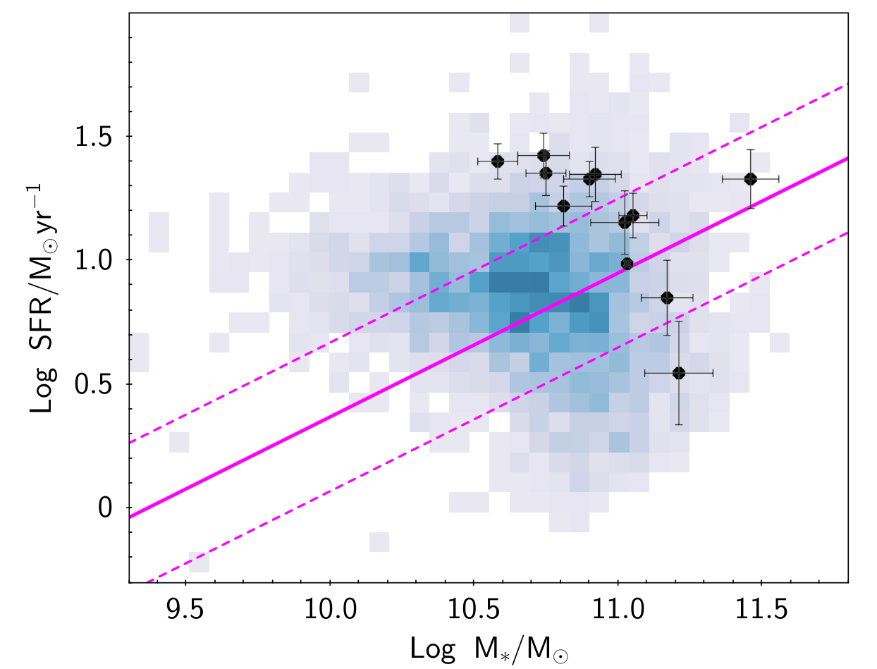
Earlier studies have shown that the 250m population is evolving rapidly over the interval (Dye et al. 2010; Dunne et al. 2011) and so we note that this sample probes an era where the galaxies were more IR luminous and gas and dust rich than those at . The sample has a narrow range of making them far more ‘typical’ of galaxies at this redshift than previous very luminous IR samples (Combes et al. 2011, e.g.). At these IR luminosities the sample should be dominated by galaxies which are forming stars under normal conditions, rather than displaying the properties of extreme star-bursts (Sargent et al. 2012). The star-formation rates are between 4–26 and stellar masses are in the range . A comparison with optically selected galaxies in the same redshift range from the GAMA survey (Driver et al. 2016; Baldry et al. 2018) is shown in Figure 1. The magenta solid and dashed lines show the ‘main sequence’ fit from Speagle et al. 2014 with dex intrinsic scatter. Most of the sample lies within the 0.3 dex scatter of the galaxy star forming main sequence at (when allowing for the measurement errors), and three sources are above the main sequence by a factor 4–6 (SDP.3132, SDP.6216, SDP.6451). It is also apparent that the 250m selection picks out the leading edge of the optical cloud of galaxies, i.e. only the most massive or highly star forming galaxies at this redshift make it above the Herschel flux limit.
Three colour optical/near-IR images of our sample from VST KIlo Degree Survey (de Jong et al. 2017) and VISTA VIKING, (Edge et al. 2013) are shown in Figure 4–15 and the optical spectra from GAMA (Baldry et al. 2018) are shown in Figure 18–23. The galaxies have a range of morphologies and colours, from compact to disk-like, with many displaying signs of disturbance such as stellar caustics and asymmetric morphology. The optical spectra predominantly show an older stellar population with superimposed emission lines indicating ongoing star formation, similar to that seen in stacked spectra in the much larger H-ATLAS sample analysed by Eales et al. 2018. One source (SDP.6216) has a clear starburst signature in the optical spectrum, and it also has the highest offset from the main sequence in Figure 1.
Metallicity is a property which affects the emission of all three gas tracers, but its most complicated effects are on CO because of a combination of non-linear FUV photon shielding effects (Pak et al. 1998; Bolatto et al. 1999; Wolfire et al. 2010).22 2 The recently explored effect of CRs only compound these difficulties (Bisbas et al. 2015; Bisbas, van Dishoeck et al. 2017). The effects on [Ci] and dust emission are more straight-forward and the abundances of these tracers are roughly proportional to metallicity. We cannot directly estimate metallicities for our galaxies as their optical spectra do not extend as far into the red as H at this redshift, i.e. there are no strong line-based methods available to measure metallicity directly (without H to correct for reddening we would not trust methods which use only the ratios of H, O[iii] and O[ii] in this dust selected sample). Fortunately, since we have a sample of massive galaxies with log , we can use the fact that the mass metallicity relation flattens at this mass in this redshift range, hence we expect these galaxies to have metallicities between 0.8–1.2 using a variety of metrics measured at this redshift (Vale Asari et al. 2009; Lara-López et al. 2010; Bothwell et al. 2016; Torrey et al. 2019). In this metallicity range we do not expect any of the molecular gas tracers to be adversely impacted because of metallicity and thus we do not consider metallicity-dependence within our sample any further.
2.2 ALMA observations and data reduction


| SB name | Date | EB | p.w.v | Phase Cal. | Flux Cal. | B.P. | |||||
| (GHz) | (min) | (mm) | (Jy) | (mJy) | |||||||
| B3 | 85.5 | 3.12.13 | Xe20 | 26 | 48.4 | 4.14 | J | Mars | J | 40 | 0.9 |
| 3.12.13 | X1032 | 26 | 48.4 | 4.14 | J | Callisto | J | ||||
| LowV (163, | 365.2 | 14.12.13 | X1644 | 26 | 50.2 | 0.84 | J | Pallas | J | 90 | 0.86 – 1.2 |
| 4104, 5347, 6418) | 26.12.14 | X2543 | 40 | 33.3 | 0.84 | J | Ganymede | J | .. | ||
| SDP.5526 | 366.8 | 21.2.14 | X5fa | 27 | 12.0 | 0.46 | J | Pallas | J | 77 | 1.25 |
| 26.12.14 | X23cb | 40 | 8.0 | 1.15 | J | Ganymede | J | .. | |||
| SDP.3132 | 362.3 | 14.12.13 | Xf8d∗ | 30 | 5.5 | 1.10 | J | Ganymede | J | 70 | 0.87 |
| 2.1.15 | X1ba4 | 39 | 5.5 | 0.70 | J | J | J | .. | |||
| 2.1.15 | X1cf1 | 39 | 5.5 | 0.72 | J | Callisto | J | .. | |||
| HighV | 363.5 | 21.2.14 | X3e5 | 28 | 35.3 | 0.64 | J | Ganymede | J | 65 | 0.84 – 1.1 |
| (1160, 2173, | 2.1.15 | X1e75 | 39 | 34.2 | 0.69 | J | Callisto | J | .. | ||
| 3366, 5323, | 2.1.15 | X2365 | 39 | 15.4 | 0.82 | J | Ganymede | J | .. | ||
| 6216, 6451) | 2.1.15 | X2606 | 39 | 34.2 | 0.91 | J | Ganymede | J | .. |
is the average rms in Jy/beam for the continuum. ∗ M.S. not used as it did not improve the overall noise level or image quality.
Choosing an observing set-up to cover both the and [Ci](3P1-3P0) lines with only Band 3 and Band 7 receivers available led to a severe restriction on the redshift of sources which could be observed in Cycle 1. Unfortunately, due to this restricted receiver choice the [Ci] (1–0) spectral window had to be placed in the wings of an atmospheric water line, thus the transmission in the [Ci] window is lower than that in the other three used for the continuum (Figure 2). The Band 3 base-bands were placed as close to the edge of the band as possible in order to maximise the transparency at the [Ci] (1–0) frequency. With a wider choice of receivers, observations with much improved sensitivity to the [Ci] (1–0) line are now possible.
Observations were made with the ALMA-12 m array in the C32-2 and C32-3 configurations for Band 3 and the C43-1/2 configuration for Band 7. This produced beam sizes (with natural weighting) of and . The coverage for the two set-ups is shown in Figure 3, where there is clearly more sensitivity on longer base-lines (smaller angular scales) in Band 7 compared to Band 3, while the Band 3 observations have relatively more short baselines (more sensitivity to extended structure). There are fewer missing short-spacings in the coverage33 3 which are always present for interferometric observations without total power measurements the CO(1–0) compared to the [Ci] (1–0) images, which results in better sensitivity to larger angular scales in the CO(1–0) maps compared to those for [Ci] and dust. The implications of this are discussed further in Section 3.3.
The Band-3 observations of the line ( GHz) were made in Dec 2013 during Cycle 1, the spectral setup consisted of four 2-GHz bandwidth spectral windows (spws): one spw with 976 MHz channel width centered at 85.4 GHz covering the line, and three spw with 31.25 MHz channel width, centered at 87.4, 87.5 and 99.3 GHz for the continuum. The total integration time was 96 minutes, giving mJy beam-1 in a 50 channel and Jy beam-1. The Band-7 observations of [Ci](3P1-3P0) and dust continuum were split across Cycles 1 and 2 over a period from December 2013–January 2015. The spectral setup again consisted of four 2-GHz bandwidth spectral windows, one with 976 MHz channel width centered on the [Ci](3P1-3P0) line ( GHz) and the other three with 31.25 MHz channel width at lower frequencies offset by -2, -12, -14 GHz from the high resolution spw. Four different central frequencies for the [Ci](3P1-3P0) spw were used, depending on the redshifts of the sources: 366.8, 365.2, 363.5 and 362.3 GHz. The total integration time was 3.9 hours giving mJy beam-1 in a 50 channel and Jy beam-1.
The 3-mm Band 3 data were reduced manually using the Common Astronomy Software Applications (CASA) v4.5 package (McMullin et al. 2007). The starting points were the observatory scripts delivered with the data, but these needed to be adapted due to early issues in Cycle 1, such as too much data being flagged in some cases and extra flagging needed in other regions. Flux calibration was from Mars and the phase/bandpass calibrator J0854+2006 was used. The two measurement sets (MS), which were observed on the same day, were concatenated before imaging having been set to a common flux scale. The spectral line cubes were created using clean in CASA in a range of channel widths in order to determine the best SNR for each source. Any emission detected was cleaned on a channel-by-channel basis. Natural weighting was used in order to maximise signal-to-noise.
The Band 7 observations were set up in four Scheduling Blocks (SBs) where the sources that could share a single tuning were grouped into a given SB. This means that the [Ci](3P1-3P0) line is not always placed in the centre of the spectral window. Occasionally both the line and neighbouring continuum spw had to be imaged together to provide a good baseline for line fitting. Due to some of these data being taking during Cycle 2, the newer CASA v4.7 was used for the reduction. Some of the MS were calibrated using the ALMA pipeline, while others were reduced manually, depending on how the data were delivered. All MS were checked and reprocessed allowing for tailoring of the calibration to the specific issues in this data-set. For example, there are several atmospheric lines which are evident in the Band 7 data and so the pipeline calibration was modified to avoid flagging the Tsys response in some cases, and to output the data-set from the pipeline after the generation of the water vapour radiometer (WVR) and calibration tables. The data were then manually processed from that stage so that the atmospheric lines could be flagged in the bandpass calibrator and the bandpass solutions interpolated in these regions. Additional manual flagging was also applied where required.
Imaging of the [Ci](3P1-3P0) line and continuum was performed using the casa task tclean with a Hogbom algorithm, using natural weighting. The dust continuum emission at GHz (rest-frame 480 GHz) was imaged using the line-free portions of the data. Images were made at full resolution () and also tapered in the -plane to increase the sensitivity to any low level extended emission. The optical diameter of the galaxies is 4–9′′, and so they are expected to be resolved in our observations. Sources above in the dirty image were masked and lightly cleaned (to 1.5).
Spectral line cubes were created using velocity channels chosen on the basis of the lines found (ranging from 30-150 ). Line emission above 3 detected in the dirty image was masked in each channel individually and cleaned down to 1.5. If the continuum emission was strong, it was subtracted from the cube using the casa task imcontsub, this was only necessary in the case of SDP.163 as in all other sources the peak continuum emission was much less than the rms in the line channels. We searched near the optical redshift for emission, also taking account of any neighbouring optical sources which may have been at a similar redshift and interacting with the main source (as turned out to be the case for four targets). The cubes were collapsed to make a moment 0 map across the velocity range where line emission was seen using the immoments task in casa.
Images are presented in Figure 4–15 and are not corrected for the variable attenuation of the primary beam over the field, being displayed instead as signal-to-noise contours.44 4 It should be noted that a source nearer to the edge of the map will have a higher flux at the same contour level compared to a source in the centre, due to the fact that the primary beam attenuation increases the noise as a function of radius from the pointing centre.
2.3 Flux measurements.
Continuum fluxes were measured on either the full resolution or tapered maps depending on the source size and morphology. For the most accurate fluxes we fitted Gaussians, using the CASA tasks imfit and gaussfit where possible, which meant using the tapered maps for the more extended sources and the full resolution maps for any point like sources. Where a source was reported to be unresolved or no size could be measured, we opted to use the peak flux, which is equivalent to that derived when fixing the size parameters to be equal to those of the beam. When a source was resolved and had a peak SNR, we used the integrated flux from the Gaussian fit, while for extended sources where a Gaussian was not a good representation, or when the SNR was less than 5, we used an aperture around the source emission (Simpson et al. 2015; Oteo et al. 2016, e.g)
When fitting fluxes using imfit or gaussfit, we used only a small region to actually solve the fit parameters as this makes the fitting less unstable. However, the flux error returned by the algorithm in casa is usually underestimated due to the presence of correlated noise in the map pixels (Condon 1997). To deal with this, we first measured , the pixel rms noise on the non primary-beam-corrected image, over a large enough region to be a true representation. We then derived the correct fractional errors on the flux output by the casa fitting task using the following equation:55 5 This is based on Condon 1997.
| (1) |
where and are the fractional error on the amplitude and integrated flux returned by the algorithm.
The amplitude error is underestimated if too small a region is used by the algorithm to determine the map rms, and so we correct this using the ratio of our own measurement of the noise to the rms used by algorithm in its determination of the errors ().66 6 In imfit one can simply supply to the task, thus overriding the noise estimate from the smaller region over which the fit is to be performed.
For the aperture measurements, we estimated the noise using the formulation in Dunne et al. 2000 which accounts for correlated noise:
where is the noise in an aperture which has pixels. is the pixel to pixel rms measured in large off-source regions of the map and is the number of pixels in the beam. This is equivalent to putting down random apertures on the map and estimating the variance of their sums (assuming the noise is Gaussian other than the beam scale correlations).
We corrected the aperture measurements for the fraction of the beam falling outside the aperture by comparing the fluxes within the same aperture placed on the phase calibrator with that returned by the imfit task in CASA, following the method outlined in Simpson et al. 2015.
Integrated line fluxes were calculated in a similar way to the continuum fluxes, either by fitting a Gaussian to the moment 0 image, or using an aperture if that was more appropriate. No thresholding was applied to the moment 0 maps to avoid biasing the fluxes. All fluxes and errors were then corrected for the primary beam attenuation using the primary beam model output by CASA during the clean stage. The integrated line intensities and other observational parameters for CO are listed in Table 3, and those for [Ci] and dust are found in Table 4.
| Source | R.A. | Dec | FWHM | |||
|---|---|---|---|---|---|---|
| (J2000) | (J2000) | ( ) | ( ) | (Jy ) | ( ) | |
| 163 | 09:05:06.19 | 02:07:02.2 | 80 | |||
| 1160 | 09:00:30.13 | 01:22:00.4 | 100 | |||
| 2173 | 08:58:49.36 | 01:27:41.4 | 50 | |||
| 3132 | 09:14:35.28 | 00:09:35.7 | 15 | |||
| 3366 | 09:04:50.10 | 00:12:03.6 | 50 | |||
| 4104.a | 09:07:07.85 | 00:00:02.4 | 60 | |||
| 4014.b | 09:07:07.82 | 00:00:05.1 | 60 | |||
| 5323 | 09:08:45.32 | 02:53:21.2 | 80 | |||
| 5347 | 09:06:58.22 | 02:02:45.73 | 80 | |||
| 5347(S) | 09:06:58.63 | 02:02:35.87 | 80 | |||
| 5526 | 09:04:44.88 | 00:20:48.2 | 50 | |||
| 6216 | 09:08:44.79 | 00:21:17.9 | 50 | |||
| 6418 | 09:04:02.15 | 01:07:58.9 | 75 | |||
| 6451 | 09:08:49.2 | 02:25:57.8 | 50 | 0 | ||
| 50 | -50 |
Each component found is listed on an individual
line. a or g next to the flux indicate whether an aperture
was used or a Gaussian fit, although where both methods could be
used they gave comparable results within the errors. indicates
the measurement was made on the tapered map. Bold font indicates
measurements with integrated flux at . Details on
individual source measurements can be found in
Section A.
SDP.5347 has two or three optical
components and it is difficult to disentangle the CO emission. The
sources appear to be merging and there is CO emission at a similar
velocity outside the optical disks which may be tidal
remnants. The first row includes emission from the three optical
components which have similar velocities. The second row (S) is
the clump of emission to the South which can be seen in
Figure 11. This southern emission is not used in any
further analysis. 6451 has very weak CO emission over a velocity
range . The first entry in the table above is
the peak flux from fitting a Gaussian to the brightest peak
coincident with the [Ci] peak. The second entry is using an aperture
which covers the same area as that used to measure the [Ci] flux in
Table 4.
| Source | R.A. | Dec | FWHM | |||||
|---|---|---|---|---|---|---|---|---|
| (J2000) | (J2000) | ( ) | ( ) | (Jy ) | ( ) | (mJy) | (m ) | |
| 163 | 09:05:06.11 | 02:07:01.9 | 150 | 837.18 | ||||
| 1160 | 09:00:30.15 | 01:22:00.2 | 50 | 840.27 | ||||
| 2173 | 08:58:49.31 | 01:27:41.3 | 30 | 840.69 | ||||
| 3132 | 09:14:35.28 | 00:09:35.7 | 20 | 843.98 | ||||
| 3132+ACA | ||||||||
| 3366.a.v1 | 09:04:50.13 | 00:12:03.6 | 100 | 840.29 | ||||
| (3366.a.v2) | 09:04:50.09 | 00:12:03.0 | 100 | .. | .. | |||
| (3366.b) | 09:04:50.21 | 00:12:01.0 | 100 | 840.29 | ||||
| 4104.a | 09:07:07.85 | 00:00:02.4 | 50 | 835.31 | ||||
| 4104.b | 09:07:07.82 | 00:00:05.1 | 50 | 835.31 | ||||
| 5323.v1 | 09:08:45.30 | 02:53:21.7 | 80 | 841.43 | ||||
| 5323.v2 | 09:08:45.30 | 02:53:21.7 | 80 | .. | .. | |||
| (5323.v3) | 09:08:45.29 | 02:53:20.9 | 80 | .. | .. | |||
| 5347.a | 09:06:58.45 | 02:02:45.2 | 80 | 849.38 | ||||
| 5347.bc | 09:06:58.22 | 02:02:47.6 | 80 | (b) | 849.38 | |||
| 5347.bc | “ ” | “ ” | 80 | (c) | 849.38 | |||
| (5347.S) | 09:06:58.56 | 02:02:39.3 | 80 | 849.38 | ||||
| 5526 | 09:04:44.88 | 00:20:48.2 | 50 | 833.32 | ||||
| 6216 | 09:04:02.15 | 00:21:17.9 | 50 | 841.44 | ||||
| (min) | 50 | .. | ||||||
| (max) | 50 | .. | ||||||
| 6418.a | 09:04:02.14 | 01:08:00.4 | 75 | 835.33 | ||||
| (6418.v1) | 75 | .. | ||||||
| 6418.v2 | 75 | .. | ||||||
| (6418.v3) | 75 | .. | ||||||
| (6418.b) | 09:04:02.37 | 01:07:58.5 | 75 | 835.33 | ||||
| 6451 | 09:08:49.49 | 02:25:57.6 | 50 | 841.44 |
The positions and fluxes of the various components
are listed with the following nomenclature: Spatially distinct
components which are identified with separate optical sources are
given letters to denote them. Kinematically distinct components in
the same source are denoted as . The components which are
used to derive the physical properties such as luminosity and gas
mass in Tables 6 and 7 are shown without
brackets, while those inside brackets are not used.
a or g
next to the flux indicate whether an aperture was used or a
Gaussian fit, although where both methods could be used they gave
comparable results within the errors. indicates the
measurement was made on the tapered map. Measurements at
are in bold.
For details on the individual entries
please see notes in Appendix A.
3132 had ACA data
taken in Cycle 7 and the inclusion of this leads to the second row
of fluxes denoted +ACA.
3366 has three components: the
main optical galaxy 3366.a has two associated velocity components,
and while the small blue companion, 3366.b, has a broad
line which overlaps the velocity profile of 3366.a.v2.
4104
(interacting pair) has spatially and kinematically resolved
components in both CO and [Ci] .
5323 has three velocity
components: north of the nucleus , south of the
nucleus ( ), and high velocity emission (Fig. 10). There is no corresponding CO
emission for the high velocity component, and we do not consider it further.
5347 ‘a,b,c’ refer to
the main optical galaxy, the satellite seen to the west within the
optical isophotes of the main galaxy with the strongest CO peak,
and the satellite visible to the north-west respectively. 5347.S
is a clump of emission to the South which overlaps in velocity
with the clump seen in CO.
6216 is an extended source with
complex continuum morphology, three continuum fluxes are
given. The first includes all the emission except for the Eastern
arm-like extension. The second is a robust minimum flux which
subtracts the compact clump discussed in Appendix A,
and does not include the Eastern extension. The third is a robust
maximum which includes all three components.
6418.a is the main
optical target, and the next three rows are the three velocity
components , the sum of which constitutes the flux for
6418.a. The smaller optical companion, 6418.b, has very low SNR
850m continuum flux but has [Ci] at the same velocity
as the 6418.a().
Spectral profiles were extracted either from the peak pixel of a point source, or from the aperture which covered the region of interest. The profiles were baseline subtracted, boxcar or Hanning smoothed in some cases and fitted with a Gaussian line profile. The profiles are shown in Figures 4- 15 and the fitted parameters are listed in Tables 3 and 4.
3 Results
We detect a total [Ci] flux above 3 for all 12 sources, for dust continuum the number is 11 and for CO we detect at this level in 10 sources. There are a wide variety of morphologies and relative luminosities. The optical images with ALMA signal-to-noise contours superimposed are shown in Figures 4–15 along with the CO and [Ci] spectral profiles. We comment in detail on each source in Appendix A.
Half of the fields contained one or more serendipitously detected high redshift dusty star-forming galaxies, identifiable as point sources with SNR and having either no optical/NIR counterpart, or a very red K-band detection in the VIKING imaging. In total 7 high redshift dusty galaxies are confidently detected at in 6 fields. A full investigation of these sources, which constitute an overdensity relative to the blank field counts of a factor 4–6 is given by Dunne et al. 2020.
3.1 Physical parameters from SED fitting
We have estimated physical parameters for the galaxies using the energy balance SED fitting code magphys, which uses libraries of optical and infrared SEDs with parameters drawn stochastically from physically motivated priors. Details of the fitting method are presented in da Cunha et al. 2008. We use extended infrared libraries which have an ISM cold temperature range of 10–30 K (Rowlands et al. 2014; da Cunha et al. 2015), as several of the sources favoured warmer ISM temperatures than allowed in the standard magphys infrared libraries. We fit the FUV–850m photometry (typically 22 or 23 bands), including an additional 7% error in quadrature to incorporate calibration, zero point and model scatter. The FUV-22m photometry is taken from the LAMBDAR catalogue (Wright et al. 2016), while the Herschel photometry is listed in Table 5. We take the IRAS scanpi (Helou et al. 1988) upper limits at 60m and use them as a constraint on the fitting. In several cases there is contamination of the SPIRE photometry from background sources at higher redshift in the Herschel beam. Sometimes the contaminant source is visible in the ALMA continuum images, other times it is evident from the 250m /350m and 350m /500m colours that another higher redshift source must be contributing to the SPIRE fluxes. We describe in Appendix B and in Dunne et al. 2020 how we estimate the range of possible contamination of the Herschel fluxes, in order to correct them. Where there is evidence for contamination, we have fitted the photometry with and without making this correction to check the impact on the SED. We find that, while in all cases making these corrections improves the fit to the SED, the changes to the estimated parameters are very small and within the original 1 uncertainties in all cases. Therefore the choice of whether to correct, or how to correct has no bearing on our findings in the next section. Our companion paper provides further detail and also investigates the wider implications of this boosting for cases where ALMA data are not present.
We show the best fit SED and parameter PDFs in Figure 18-23. Alongside the best-fit SED in red we also show 200 of the SEDs which are strongly contributing to the PDFs. The median parameters and their uncertainties are listed in Table 6.
| Source | ||||||||||||
|---|---|---|---|---|---|---|---|---|---|---|---|---|
| 163 | 73.9 | 20.7 | 102.1 | 24.1 | 107.6 | 7.3 | 50.7 | 8.1 | 23.9 | 8.5 | 3.05 | 0.34 |
| 1160† | 49.8 | 17.5 | 57.1 | 19.7 | 48.4 | 7.2 | 32.4 | 8.1 | 21.6 | 8.7 | 0.54 | 0.12 |
| 2173† | 59.0M | 34.0 | 68.0M | 38.0 | 46.2 | 6.5 | 21.4 | 7.5 | 11.1 | 7.8 | 0.74 | 0.20 |
| 3132 | 64.3M | 26.5 | 65.1M | 20.0 | 40.6 | 6.4 | 23.6 | 7.4 | 13.1 | 7.8 | 0.95 | 0.29 |
| 3366† | 19.7 | 24.5 | 114 | 37.6 | 40.3 | 7.3 | 26.3 | 8.0 | 16.5 | 8.8 | 0.42 | 0.019 |
| 4104† | 77.9 | 17.6 | 53.3 | 26.4 | 46.2 | 7.2 | 28.3 | 8.1 | 12.1 | 8.8 | 0.92 | 0.24 |
| 5323 | .. | .. | .. | .. | 28.6 | 7.1 | 30.0 | 8.0 | 9.6 | 8.4 | 0.89 | 0.24 |
| 5347† | 33.0 | 41.2 | 68.0 | 17.7 | 32.7 | 7.5 | 29.8 | 8.2 | 17.2 | 8.7 | 1.84 | 0.35 |
| 5526 | 62.0M | 32.6 | 56.9M | 40.7 | 31.2 | 7.3 | 20.0 | 8.2 | 10.7 | 8.5 | 1.11 | 0.27 |
| 6216 | 35.0M | 36.6 | 34.0M | 40.7 | 36.2 | 7.3 | 19.9 | 8.1 | 3.8 | 8.8 | 1.49 | 0.25 |
| 6418† | 40.4M | 19.8 | 27.0M | 33.3 | 31.6 | 7.3 | 18.5 | 8.0 | 16.6 | 8.4 | 1.06 | 0.32 |
| 6451† | 69.4 | 41.7 | 59.5 | 47.8 | 33.7 | 7.3 | 29.7 | 8.2 | 19.5 | 8.6 | 0.88 | 0.19 |
Notes: Fluxes are all in mJy. † indicates that there is evidence for contamination of these Herschel fluxes by high-z SMG in the beam. Before SED fitting we subtract from these fluxes the estimated contamination from high-z SMG listed in Table 9. See Appendix B for details. M indicates a PACS flux re-measured from the DR1 maps.
| Source | Log | Log | Log | Log | Log | Log | log sSFR | |
|---|---|---|---|---|---|---|---|---|
| () | () | () | ( ) | ( ) | ( ) | () | (K) | |
| 163 | ||||||||
| 1160† | ||||||||
| 2173† | ||||||||
| 3132 | ||||||||
| 3366† | ||||||||
| 4104† | ||||||||
| 5323 | ||||||||
| 5347† | ||||||||
| 5526 | ||||||||
| 6216 | ||||||||
| 6418† | ||||||||
| 6451† |
Notes on Luminosities 3366: [Ci] is from 3366.a.v1 only. 4104: the sum of both members of the pair as measured with the missing channels. 5323: [Ci] is the sum of the two velocity components and from Table 4. 5347: sum of the massive galaxy and the two satellites which have dust and/or [Ci] and CO emission (5347a–c in Table 4). 6216: flux at 850m is that from the main disk including the compact clump discussed in Appendix. A. 6418: [Ci] flux is only that of the component in the main galaxy. Notes on magphys parameters: † Fits use sub-mm fluxes from Table 5 which are then corrected for high-z contamination where required (see Appendix B). The differences in the fitted parameters using fluxes which are corrected for estimated contamination by dusty high redshift galaxies detected by ALMA within the SPIRE beam is well within the error and so the consideration of contamination has a negligible effect on the properties derived here. The dust mass estimates using the ALMA data in addition to the Herschel fluxes are considerably lower than when using the Herschel data alone.
3.2 Kinematics
The kinematics of the sources were more complex than anticipated in many cases. In seven cases, there is a single optical galaxy where CO and [Ci] have similar line-widths and velocities and similar morphology.77 7 As far as we can tell with the resolution differences between 85 GHz and 365 GHz. We call these the Simple Kinematic (SK) sources. The other five sources have disturbed kinematics (DK), four of which (SDP.3366, SDP.4104, SDP.5347, SDP.6418) have a smaller neighbouring optical source which shows either CO, [Ci] or both at a similar velocity, indicating tidal interaction. SDP.5323 has a very complex velocity field in [Ci] with three components, and may be hosting an outflow or be involved in an interaction with a satellite.
3.3 Gas and dust morphology
The ALMA Band 7 data provide 850m (rest-frame 620m ) dust and [Ci] line imaging at a common angular resolution () and with the same () coverage, so that morphological comparisons between the [Ci] and dust are meaningful. The CO imaging is at a very different frequency, which translates into different sensitivity to spatial scales within the interferometer. The smallest spatial scales probed are set by the longest baselines, and the synthesised beam with natural weighting gives a physical resolution of 10 kpc for CO(1–0), and 4 kpc for [Ci] (1–0) and dust. The CO is unresolved or very marginally resolved in all sources, apart from SDP.5347, where there appears to be some large scale tidal debris.
The Maximum Recoverable Scale (MRS) for the CO imaging is of order 20′′(100 kpc), while for [Ci] and dust it is only ′′(25 kpc), where we are quoting the quantity ).88 8 At the time of the Cycle 1 call, the proposal guide gave an MRS of 25′′and 7.1′′respectively for the two bands. This, plus the severe restriction on observing time for Cycle 1 meant that we did not request ACA data in the first instance. The optical diameter of the galaxies ranges from 4-7′′(20–35 kpc at this redshift), and we did not expect the molecular gas to be distributed smoothly on scales this large. However this may not be so for the CI-bright distribution as CO-poor gas will be preferentially be at larger galactocentric distances because of metallicity gradients and/or lower gas densities allowing FUV radiation and/or cosmic rays to shift the relative abundance towards higher values in outer regions. Moreover cold dust is typically found well-beyond optical disks and even well-concomitant with HI (Alton et al. 1998; Thomas et al. 2002a; Smith et al. 2016; Casasola et al. 2017). A subsequent ACA proposal to image those sources with the most extended emission was approved in the Cycle 7 supplementary call, however, only one source had data taken before ALMA ceased operations in March 2020. This source (SDP.3132) shows a small (10 percent) increase in [Ci] flux once the ACA data are included, but a much larger (60 percent) increase in the dust flux, from to .99 9 While the fractional increase is large, the uncertainties mean that the actual difference is not statistically very significant. This is not unexpected as the fainter dust continuum is affected more by the filtering effect of the missing short spacings, because there is no frequency dependence in the emission morphology. Other sources which appear to have diffuse dust emission (predominantly the disks which are face-on, SDP.2173, SDP.6216, SDP.6418) may also have substantial fractions of the dust flux resolved out, although there is no indication of anything larger than the effect on SDP.3132 given that none of these sources are outliers in the [Ci] –dust or CO–dust relations.
Ultimately, only higher sensitivity (u,v)-matched imaging of CO(1-0), dust continuum and [Ci] line emission can resolve these issues, an observing setup that is not trivial, especially between CO(1-0) and [Ci] (1-0) lines, given their very different frequencies. Still, should significant tracer brightness be resolved out by our current imaging setup, this will certainly impact any extended [Ci] line and dust continuum distribution much more than that of CO(1-0) because of the differential (u,v) coverage between the low and high frequency observations filtering-out extended emission from the high-frequency tracers (see Figure 3).
Within the limitations of the data (both in terms of resolution, coverage, and signal-to-noise), we can say that three of the sources show evidence for some difference between the dust and [Ci] distributions. SDP.5323 has a very compact dust morphology centered on the nucleus while the [Ci] is found in two lobes outside of the dust core. The CO appears to be more similar to the dust than to the [Ci] but the poorer angular resolution and SNR of the CO imaging means we cannot be confident. SDP.6216 has centrally concentrated [Ci] emission while the continuum morphology is diffuse and complex. SDP.6418 has dust emission at low level near to the optical centre while the [Ci] is located in several clumps at different velocities. The [Ci] is distributed over a much wider area than the dust, although the SNR is very low for the dust and so differences here could just be due to there being a diffuse distribution and low SNR.
In summary, there are some very interesting morphological differences between the [Ci] and dust, however, the SNR is not high enough for us to be confident that these are real in all cases. The CO(1-0) observations are at a very different angular resolution and do not provide much information on the morphology. To undertake a meaningful morphological comparison of the three tracers requires further observations to (a) improve the sensitivity in all three tracers and (b) crucially match the resolution and the () coverage between the Band 3 and Band 7 observations.
3.4 Relationships between the tracers
The fluxes which are not in parentheses in Tables 3 and 4 are used to estimate the line luminosities (Solomon & Vanden Bout 2005) and rest-frame 850m monochromatic luminosity as follows:
| (2) |
Where is the velocity-integrated flux density in Jy , is the luminosity distance in Mpc and is the rest frequency of the transition in GHz.
| (3) |
where is the luminosity distance, is the observed flux at 353 GHz, and is the K-correction to rest-frame 850m , defined as
| (4) |
Here , is the luminosity weighted dust temperature (from an isothermal fit to the SED) with . K-corrections for this sample ranged from 2.6–3.0, therefore making this extrapolation to rest frame 850m in order to be consistent with the literature (Scoville et al. 2016) does not add significant uncertainty to what we are doing. These luminosities are reported in Table 6.
The correlations between the three observables, , and are shown in Figure 16, along with the best linear 1:1 fit in order to visually compare the consistency of the various tracers. The two sources which have alternative [Ci] estimates (SDP.4104 and SDP.6418) are shown as cyan and pink circles with the two values joined by a dashed line. The choice of which [Ci] flux to use has no material impact on the conclusions or results. This sample is too small and has too limited a dynamic range in luminosity to make meaningful fits to these relationships, and we defer this process to a much more comprehensive analysis which combines this sample with others from the literature (Dunne et al. in prep). Suffice to say that the trend noted here, for [Ci] –dust to have the lowest scatter, is borne out by the analysis on a much larger sample of sources.


We also show the ratios of the tracers as a function of sSFR in the right column of Figure 16. The top row shows the / ratio which shows no apparent trend. The middle row shows , with the average values for the Milky Way (Frerking et al. 1989) and high-z QSO (Walter et al. 2011) shown as the grey dot-dashed (lower) and dotted (upper) horizontal lines respectively. With two exceptions (SDP.6418 and SDP.6451), the galaxies fall in a reasonably tight band with a spread of dex, and a trend to lower values of with increasing sSFR. The two exceptions have much higher for their sSFR, although the significance of the offset would need to be confirmed with more sensitive CO observations. The bottom row shows / , which has the smallest dispersion. The very highest sSFR galaxies have the lowest / ratios, but given the sample size and error bars there is no significant trend.
The means and medians (in brackets) and 1 ranges for the ratios are: log , and . The relationship with the least variance is – which implies that these two tracers are better correlated with each other than either of them are with CO. We will return to the implications of these relationships for calibrating the tracers in Section 4.
3.4.1 Potential CO-‘dark’ galaxies
The two sources (SDP.6418 and SDP.6451) which are outliers in the [Ci] –CO relationship (Figure 16), have very weak CO emission despite being detected both in dust and [Ci] . The sources are unremarkable in the [Ci] –dust relationship indicating that this seems to be a deficiency in CO relative to the other tracers rather than an enhancement in [Ci] . There is nothing particularly special about these sources, their stellar masses are log , and neither show evidence for an AGN in the optical spectra, using the criteria of Lamareille 2010; they have O[ii] flux greater than O[iii], and O[iii] is generally weak. As pointed out in Section 3.3, any filtering of flux on extended scales is going to affect [Ci] more than CO and so this cannot be an explanation for the high [Ci] /CO ratio. More data would be needed to confirm this unusual / ratio, both to increase the sensitivity in the line observations and to match the resolution between the tracers. The ratio of line luminosity / () in these galaxies ranges from , using the measured CO fluxes which are only 2 significance. Using a 3 upper limit on the CO flux gives a lower limit of for SDP.6418 and SDP.6451 respectively. The average value in Milky Way clouds is (Frerking et al. 1989), while the average value seen in QSO is (Walter et al. 2011).
Understanding how reasonably normal star forming galaxies like these can be so deficient in CO is very important for understanding the C/CO dependencies in the ISM. One mechanism for reducing CO emission relative to [Ci] is cosmic ray destruction of CO molecules volumetrically in the clouds, something discussed at length in Bisbas et al. 2015; Glover & Clark 2016; Bisbas et al. 2017; Papadopoulos et al. 2018. The more recent works show that conditions do not have to be extreme in terms of () in order to produce a high abundance ratio, providing that the average gas density is moderate to low. We note that it is not unheard of to find global reservoirs dominated by low-density gas, even in vigorous SF environments, and can be the result of coherent SF feedback on the gas reservoir. This may indeed be so for Arp 193, the most extreme ULIRG in the local Universe after Arp 220, where only small () gas mass fractions at are inferred from multi-J CO, 13CO, HCN and CS observations (Papadopoulos et al. 2014). We will discuss the line luminosity ratio and how observations compare to theory in more detail with a much larger sample in (Dunne et al. in prep).1010 10 An example of a very low / ratio in a local LIRG has been recently reported by Michiyama et al. 2020, which further indicates the need to better study a diverse range of galaxies with ALMA in order to understand the effects of the ratio on global tracers.
Finally we note that since: a) C-rich gas may extend further out in galactocentric distance than CO-rich gas, and b) differential ()-sampling will filter out extended [Ci] line emission more than the much-lower frequency CO(1-0) line, we expect that ()-matched CO, [Ci] line imaging of this sample will not only preserve our results about CO-‘dark’ galaxies, but it may even ‘push’ some other galaxies towards a global CO-deficient/ [Ci] -rich state by revealing more [Ci] line emission over larger areas. In that regard, ACA imaging observations, that include total power, of the CO(1-0), [Ci] (1-0) and dust continuum, can provide a definitive test.
4 Calibration of gas mass.
We estimate the molecular gas mass of the galaxies in our sample using each of the tracers in turn following the method described in detail in Dunne et al. in prep. We differentiate between - the mass of molecular hydrogen, and - the mass of molecular gas including a factor 1.36 contribution from He. Briefly, to determine we need a value for the calibration parameter for each tracer: for [Ci] we need to know the abundance , for CO we need the factor and for dust we need to know the gas-to-dust ratio . The molecular hydgrogen gas mass (in units) then depends on these calibration factors as follows:1111 11 Other literature works define quantities such as and which are simply related to our calibration factors, and will be presented at the end of this section.
| (5) |
The conversion of to also requires an estimate of , which is an excitation function. This is not a strong function of kinetic temperature (see Papadopoulos et al. 2004, Dunne et al. in prep) and so we will simply take a single value as is common in the literature. We choose to use the value based on the more detailed analysis of a larger sample in Dunne et al. in prep. The dust mass is calculated from using the mass weighted dust temperature from the magphys fits and assuming a value for the dust mass opacity at 850m of which is consistent with the results from Planck Collaboration XIX 2011 (see Dunne et al. in prep for more detailed descriptions of the dust opacity factors).
For each source, we have four unknowns, , , , , and three observables , , . If we had an independent measure of the true , then the observed values of , and would provide direct estimates of the three calibration parameters, , and . But, of course, we do not know the value of , so we need to use a probabilistic argument based on the fact the observations do provide constraints on the relative values of , , and for each source.
For each source there is a set of self-consistent calibration factors which link the observed , , to the true , with a common, but unknown constant factor. We can write down the products and ratios of these calibration factors in terms of the observed luminosity ratios:
| (6) |
From our parallel study of a larger sample of 72 sources all with CO, [Ci] and dust measurements (Dunne et al. in prep), we have measured the intrinsic variance for each pair of factors in Eqn. 6. We assume that the covariance between the calibration factors is zero, and use the three pair variances to estimate the intrinsic variance of each individual calibration factor, the population standard deviations of these are denoted , and for , and respectively.
With the constraints given by Eqn 6 we are in a position to determine self-consistent values for each of the calibration factors, , and , except for one thing: we do not have any independent measure of the gas mass on which to tie the normalisations of the our calibration (4 unknowns but only 3 measurements). We therefore have to assume a sample average for one of the unknown calibration factors, but having done so the relative values of all three will be optimised, and it is trivial to re-scale the solutions to a different normalisation if desired. We choose to normalise to a sample mean which is the Milky Way value for Hydrogen (no He) from the THEMIS dust framework (Jones 2018).1212 12 More precisely the combination of / we use is 2077, which is the quantity that calibrates dust emission to gas mass. This is equvialent to in S.I. units, where is the dust opacity at 850m per H atom.
Dunne et al. in prep use their sample of 72 sources which have observations for all three gas tracers1313 13 That sample includes the 12 galaxies from this analysis. to estimate the mean values of and . This gives us the 3 calibration factors normalised to the Milky Way value of . Using these mean values together with the population standard deviations, , , , we can estimate the probability of finding a particular set of calibration factors for any given source. Using to denote the logarithms of the three calibration factors, we can write the means and effective standard deviations as , and respectively, where the effective standard deviation is the intrinsic scatter on each parameter added in quadrature to the measurement error for that gas tracer. Assuming these follow Gaussian distributions, the probability of finding calibration factors for any source is given by
| (7) |
For any given source, we use the observed luminosity ratios in Eqn. 6, to fix the ratios of calibration factors, and choose the common scaling factor that maximises the probability in equation 7. The resulting optimised parameters are listed in Table 7, and shown in Figure 17, while the average values for the sample are listed in Table 8. By design, each tracer for a given source will produce the same gas mass when used in Eqn. 5. The errors are quoted as the values which give . We list these gas masses in Table 7 along with the gas fraction, , which is defined as . 1414 14 If we use the median calibration factors from the sample, listed in Table 8, to derive gas masses from each tracer independently (as one would do if only one measurement were available) there can be some dispersion in the three gas mass estimates depending on how far away a particular source lies in the distribution from the median. For most sources, the mass difference between any pair of tracers is within dex, except for the two sources with high (SDP.6418 and SDP.6451).
| Source | Log | |||||||
|---|---|---|---|---|---|---|---|---|
| [ ] | [] | [ ] | [] | [Gyr] | ||||
| 163 | 17.9 | 2.4 | ||||||
| 1160 | 14.9 | 1.1 | ||||||
| 2173 | 16.4 | 0.9 | ||||||
| 3132 | 19.9 | 0.24 | 0.7 | |||||
| 3366 | 15.7 | 0.06 | 2.8 | |||||
| 4104 | 21.4 | 0.19 | 0.9 | |||||
| 4104c | 18.4 | 0.21 | 1.0 | |||||
| 5323 | 20.4 | 0.13 | 1.1 | |||||
| 5347 | 21.5 | 0.22 | 5.7 | |||||
| 5526 | 23.3 | 0.14 | 1.7 | |||||
| 6216 | 26.0 | 0.32 | 0.7 | |||||
| 6418 | 17.1 | 0.20 | 1.0 | |||||
| 6418t | 15.3 | 0.28 | 1.5 | |||||
| 6451 | 13.0 | 0.26 | 0.9 | |||||
Gas mass in using the optimised calibration method described in Section 4. The optimised calibration parameter for each gas tracer, , and . Gas fraction defined as /( + ), using the value of from the magphys fitting in Table 6. Gas depletion timescale, /SFR, in Gyr. SDP.4104c uses the [Ci] fluxes corrected for flagged channels within the line profile as described in Appendix A. SDP.6418t uses all three of the [Ci] velocity components, as opposed to just the component.
| Parameter | mean | median | |
|---|---|---|---|
| () | 0.1 | 1.6 | |
| 0.1 | 1.7 | ||
| 0.5 | 2.8 | ||
| 0.7 | 2.8 | ||
| 16 | 111 | ||
| 16 | 118 |
The sample averages for the calibration parameters, using the optimisation procedure described in Section 4. The first line represents the values using the conservative [Ci] estimates for 6418 and 4104. The second row includes all the velocity components for 6418 and corrects the [Ci] flux for 4104 for the missing channels as described in the text. The errors quoted on the mean are the 16th and 84th percentiles representing the scatter. is the formal error on the mean (i.e. times the scatter.
5 Discussion
5.1 Calibration factors
We now place the values of our gas calibration factors into context with other recent work and other nomenclature for describing them.
We find that the mean and standard deviation for , which is similar to the values found in clouds in the Milky Way (Frerking et al. 1989) and to the recent determination of using GRB/QSO absorber systems using is a totally independent method (Heintz & Watson 2020). Several authors have adopted the use of an emprical quantity , with similar units of to that of , which is used as standard in extragalactic studies. is related to carbon abundance, as follows, where we now include a factor of 1.36 for He:
Thus for our average and , we find that .
The only other source which has an estimate of independent of a blind assumption on the value of is the AGN influenced CND region of NGC 7469, for which Izumi et al. 2020 find a value of , which is equivalent to . They attribute their much higher value of to the effects of an X-ray dominated region (XDR) on the ISM, which increases the [] ratio. High values for have also been inferred for other extreme sources in the high redshift universe such as QSO (Walter et al. 2011), however in these cases an assumption is made that in such sources, which then produces a higher compared to what would be inferred using a standard . The Izumi et al. 2020 work is novel because the calibration factors are estimated using a dynamical mass estimate for from very well sampled ALMA data. A comprehensive comparison of calibration factors with those in the literature is undertaken in Dunne et al. in prep.
We find an average , not including He,1515 15 To compare to other work which does include He and heavier elements, our values should be multiplied by 1.36. which is typical of star forming galaxies with an ISM dominated by self-gravitating clouds (Papadopoulos et al. 2012a; Bolatto et al. 2013; Sandstrom et al. 2013).
While we began with a prior that the gas-to-dust ratio would be similar to that in the Milky Way (given these are massive, metal rich star-forming galaxies), our method allows the to vary slightly in order to maximise the likelihood when considered along with the other two gas tracers. With this we find an average with a range of for individual sources ranging from 60–260, as expected for such a sample. Once again this does not include the contribution from He. It is now common to refer to the calibration between dust luminosity and gas mass as , following the work of Scoville et al. 2014; Scoville et al. 2016. This is defined as = / with units of , where now He is included in the definition of . We describe this parameter and its measurements in the literature in great detail in Dunne et al. in prep, but here just note that it is related to (assuming our and including a factor 1.36 for He) as:
where is the mass-weighted dust temperature, commonly assumed by Scoville et al. 2016 and others to be K in the sources they studied (typically high redshift star forming galaxies). Our empirically derived , using the optimal gas mass calculated using the above method, is . For our average and a K (which agrees well with the results of our magphys SED fits), we find a comparable value of . This compares with the value initially suggested by (Scoville et al. 2016) of and more recent literature studies which indicate (Orellana et al. 2017; Hughes et al. 2017; Kaasinen et al. 2019).
Overall, this sample of 250m selected galaxies at have calibration factors for CO(1–0), [Ci] (1–0) and dust which are comparable to normal spiral star forming galaxies in the local Universe, and conditions in the Milky Way.
5.2 Gas fractions and evolutionary status.
The mean gas fraction for the sample is where the error is the 1 standard deviation. This narrow range is rather surprising as 250m selection from H-ATLAS at produces samples with a huge range of gas fraction (0.1-0.9), and a mean value of (Clark et al. 2015). This selection was volume limited and dust mass selected, and was therefore dominated by lower mass, blue and Hi rich galaxies. In contrast, Figure 1 suggests that by H-ATLAS is only sensitive to the most massive dust sources, which presumably restricts the range of gas fractions, assuming that the anti-correlation between gas fraction and stellar mass holds also at (De Vis et al. 2017; Saintonge et al. 2017). At a given stellar mass, the gas fractions we find at are significantly higher than those found in the local Universe by the xCOLD GASS survey (Saintonge et al. 2017), who find for galaxies in our stellar mass range. However, in terms of specific star formation rate, the scaling found by xCOLD GASS seems to hold at , where for the expectation is , while at log this increases to . Thus the increased sSFR 3.9 Gyr in the past is completely consistent with the extra gas available without any changes to the efficiency of how it is converted into stars. This is noteworthy since the observables providing the measures of gas fraction (CO, [Ci] and dust) and sSFR (UV–optical SED) are completely independent in this study.
It is common in the literature for authors to define a gas depletion timescale (also the inverse of the star formation efficiency) as , which is a crude way of measuring the relative speed at which the current molecular reservoir is being converted into stars. We list this value for our sources in Table 7. There are limitations to this idea, principally that neither nor SFR are fixed quantities, being only a snapshot of the molecular mass at the observed epoch, and SFR being only the current SFR (averaged over Myr). The SFR will decline as the gas is consumed (thus is a lower limit to any physical depletion timescale), while in addition more gas may be accreted at later times, from either the cosmic web, mergers or simply the infall of atomic gas from the outer regions of the disk. The median of this quantity Gyr where the error is the 16-84th percentile range. This is consistent with the range of in the most massive gas-rich galaxies today, which is 1–1.6 Gyr over the same mass range as our sample (Saintonge et al. 2017). The time elapsed from to is 3.9 Gyr, which means that all of these galaxies would be passive today if they continued to form stars at the same rate without fresh gas supply. Certainly there must be some transformation from dust and gas rich galaxies at z=0.35 to passive galaxies today (Dunne et al. 2011; Beeston et al. 2018), but it is not plausible that all of them will become passive further high-lighting the limitations of the simple parameter.
6 Conclusions
We present ALMA observations of sub-mm dust continuum at 850, and [Ci](3P1-3P0) for a complete and volume limited sample of 12 sources selected at 250m from the H-ATLAS survey. We detected dust and either CO or [Ci] in all of the targets, finding:
- •
While the galaxies in the sample are reasonably ‘normal’ in terms of their and sSFR at these redshifts, a very high proportion (40 percent) of the sample are found to be interacting or kinematically disturbed systems. The interactions are mostly minor mergers, and hence maybe it is not surprising that they do not induce major star formation events.
- •
There is a large variety of morphology in the gas and dust, and in some cases the [Ci] and dust do not appear to have the same spatial structure. The CO resolution is too poor to allow a spatial comparison but kinematically there are also differences between [Ci] and CO in the most disturbed systems.
- •
The range of / in these sources is very large, covering the full range observed in local clouds in the Milky Way up to those seen in high-z QSO. We find two potential CO-‘dark’ candidates, detected in [Ci] and dust but not in CO.
- •
We estimate the gas calibration parameters, , and for each source using a likelihood approach. The sample averages are: Carbon abundance (required to calibrate [Ci] as a gas tracer) , while and , where we quote the sample log means and 16-84th percentile ranges. These factors do not include a correction for He. The starting assumption is that the average is similar to that for the Milky Way in these metal-rich massive galaxies. In other commonly used calibration units, which do account for He, these translate to and .
- •
The gas fractions in these galaxies range from 0.06–0.32, with an average of and a scatter of 0.07. This is a very small range of gas fraction, which is surprising given the very diverse galaxies in a volume limited 250m selected sample at .
We conclude this work by noting the supreme importance of (u,v)-matched imaging in all three prime gas mass tracers explored here, in order to fully and accurately reveal the similarities and differences of their distributions in galaxies. ALMA+ACA+(total power) imaging could provide the key for such comparisons in the future, by allowing the most unbiased imaging for the high-frequency [Ci] lines and sub-mm dust continuum.
Data Availability
The data underlying this article are publicly available from the ALMA archive http://almascience.eso.org/aq/ using the project code 2012.1.00973.S.
Acknowledgements
The authors thank the anonymous referee for their time in helping to improve the manuscript. LD thanks P. Papadopoulos for superb cooking, enlightening conversations and a careful proof-read and improvement of the draft manuscript. LD and SJM acknowledge support from the European Research Council Advanced Investigator grant, COSMICISM and Consolidator grant, COSMIC DUST. HLG acknowledges support from the European Research Council Consolidator grant, COSMIC DUST. This paper makes use of the following ALMA data: ADS/JAO.ALMA#2012.1.00973.S. ALMA is a partnership of ESO (representing its member states), NSF (USA) and NINS (Japan), together with NRC (Canada), MOST and ASIAA (Taiwan), and KASI (Republic of Korea), in cooperation with the Republic of Chile. The Joint ALMA Observatory is operated by ESO, AUI/NRAO and NAOJ. The National Radio Astronomy Observatory is a facility of the National Science Foundation operated under cooperative agreement by Associated Universities, Inc. The Herschel-ATLAS is a project with Herschel, which is an ESA space observatory with science instruments provided by European-led Principal Investigator consortia and with important participation from NASA. The H-ATLAS web-site is http://www.h-atlas.org. GAMA is a joint European-Australasian project based around a spectroscopic campaign using the Anglo- Australian Telescope. The GAMA input catalogue is based on data taken from the Sloan Digital Sky Survey and the UKIRT Infrared Deep Sky Survey. Complementary imaging of the GAMA regions is being obtained by a number of independent survey programs including GALEX MIS, VST KIDS, VISTA VIKING, WISE, Herschel-ATLAS, GMRT and ASKAP providing UV to radio coverage. GAMA is funded by the STFC (UK), the ARC (Australia), the AAO, and the participating institutions. The GAMA website is: http://www.gama-survey.org/. This publication has made use of data from the VIKING survey from VISTA at the ESO Paranal Observatory, programme ID 179.A-2004. Data processing has been contributed by the VISTA Data Flow System at CASU, Cambridge and WFAU, Edinburgh.
References
- Alaghband-Zadeh et al. (2013) Alaghband-Zadeh S., et al., 2013, MNRAS, 435, 1493
- Alton et al. (1998) Alton P. B., et al., 1998, A&A, 335, 807
- Baldry et al. (2018) Baldry I. K., et al., 2018, MNRAS, 474, 3875
- Beeston et al. (2018) Beeston R. A., et al., 2018, MNRAS, 479, 1077
- Bisbas et al. (2015) Bisbas T. G., Papadopoulos P. P., Viti S., 2015, ApJ, 803, 37
- Bisbas et al. (2017) Bisbas T. G., van Dishoeck E. F., Papadopoulos P. P., Szűcs L., Bialy S., Zhang Z.-Y., 2017, ApJ, 839, 90
- Boland & de Jong (1982) Boland W., de Jong T., 1982, ApJ, 261, 110
- Bolatto et al. (2013) Bolatto A. D., Wolfire M., Leroy A. K., 2013, ARA&A, 51, 207
- Bothwell et al. (2016) Bothwell M. S., Maiolino R., Peng Y., Cicone C., Griffith H., Wagg J., 2016, MNRAS, 455, 1156
- Bothwell et al. (2017) Bothwell M. S., et al., 2017, MNRAS, 466, 2825
- Bourne et al. (2016) Bourne N., et al., 2016, MNRAS, 462, 1714
- Bourne et al. (2019) Bourne N., Dunlop J. S., Simpson J. M., Rowlands K. E., Geach J. E., McLeod D. J., 2019, MNRAS, 482, 3135
- Casasola et al. (2017) Casasola V., et al., 2017, A&A, 605, A18
- Cavuoti et al. (2015) Cavuoti S., et al., 2015, MNRAS, 452, 3100
- Chapman et al. (2005) Chapman S. C., Blain A. W., Smail I., Ivison R. J., 2005, ApJ, 622, 772
- Clark et al. (2015) Clark C. J. R., et al., 2015, MNRAS, 452, 397
- Clark et al. (2019) Clark C. J. R., et al., 2019, MNRAS, 489, 5256
- Combes et al. (2011) Combes F., García-Burillo S., Braine J., Schinnerer E., Walter F., Colina L., 2011, A&A, 528, A124
- Condon (1997) Condon J. J., 1997, PASP, 109, 166
- Crocker et al. (2019) Crocker A. F., et al., 2019, ApJ, 887, 105
- De Vis et al. (2017) De Vis P., et al., 2017, MNRAS, 464, 4680
- Downes & Solomon (1998) Downes D., Solomon P. M., 1998, ApJ, 507, 615
- Driver et al. (2011) Driver S. P., et al., 2011, MNRAS, 413, 971
- Driver et al. (2016) Driver S. P., et al., 2016, MNRAS, 455, 3911
- Dunne & Eales (2001) Dunne L., Eales S. A., 2001, MNRAS, 327, 697
- Dunne et al. (2000) Dunne L., Eales S., Edmunds M., Ivison R., Alexander P., Clements D. L., 2000, MNRAS, 315, 115
- Dunne et al. (2011) Dunne L., et al., 2011, MNRAS, 417, 1510
- Dunne et al. (2020) Dunne L., Bonavera L., Gonzalez-Nuevo J., Maddox S. J., Vlahakis C., 2020, MNRAS, 498, 4635
- Dye et al. (2010) Dye S., et al., 2010, A&A, 518, L10
- Eales et al. (2010) Eales S., et al., 2010, PASP, 122, 499
- Eales et al. (2018) Eales S., et al., 2018, MNRAS, 473, 3507
- Edge et al. (2013) Edge A., Sutherland W., Kuijken K., Driver S., McMahon R., Eales S., Emerson J. P., 2013, The Messenger, 154, 32
- Frerking et al. (1989) Frerking M. A., Keene J., Blake G. A., Phillips T. G., 1989, ApJ, 344, 311
- Glover & Clark (2016) Glover S. C. O., Clark P. C., 2016, MNRAS, 456, 3596
- Griffin et al. (2010) Griffin M. J., et al., 2010, A&A, 518, L3
- Heintz & Watson (2020) Heintz K. E., Watson D., 2020, ApJ, 889, L7
- Helou et al. (1988) Helou G., Khan I. R., Malek L., Boehmer L., 1988, ApJS, 68, 151
- Hopkins et al. (2013) Hopkins A. M., et al., 2013, MNRAS, 430, 2047
- Hughes et al. (2017) Hughes T. M., et al., 2017, MNRAS, 468, L103
- Israel (2020) Israel F. P., 2020, A&A, 635, A131
- Israel & Baas (2002) Israel F. P., Baas F., 2002, A&A, 383, 82
- Israel et al. (2006) Israel F. P., Tilanus R. P. J., Baas F., 2006, A&A, 445, 907
- Ivison et al. (2011) Ivison R. J., Papadopoulos P. P., Smail I., Greve T. R., Thomson A. P., Xilouris E. M., Chapman S. C., 2011, MNRAS, 412, 1913
- Izumi et al. (2020) Izumi T., et al., 2020, arXiv e-prints, p. arXiv:2006.09406
- Jansen (1995) Jansen D. J., 1995, PhD thesis, Leiden Observatory, Leiden University, P.O. Box 9513, 2300 RA Leiden, The Netherlands
- Jiao et al. (2017) Jiao Q., Zhao Y., Zhu M., Lu N., Gao Y., Zhang Z.-Y., 2017, ApJ, 840, L18
- Jiao et al. (2019) Jiao Q., et al., 2019, ApJ, 880, 133
- Jones (2018) Jones A. P., 2018, arXiv e-prints,
- Kaasinen et al. (2019) Kaasinen M., et al., 2019, ApJ, 880, 15
- Kamenetzky et al. (2014) Kamenetzky J., Rangwala N., Glenn J., Maloney P. R., Conley A., 2014, ApJ, 795, 174
- Keene et al. (1985) Keene J., Blake G. A., Phillips T. G., Huggins P. J., Beichman C. A., 1985, ApJ, 299, 967
- Keene et al. (1997) Keene J., Lis D. C., Phillips T. G., Schilke P., 1997, in van Dishoeck E. F., ed., IAU Symposium Vol. 178, IAU Symposium. pp 129–139
- Kelvin et al. (2012) Kelvin L. S., et al., 2012, MNRAS, 421, 1007
- Krips et al. (2016) Krips M., et al., 2016, A&A, 592, L3
- Lamareille (2010) Lamareille F., 2010, A&A, 509, A53
- Langer (1976) Langer W., 1976, ApJ, 206, 699
- Lara-López et al. (2010) Lara-López M. A., Bongiovanni A., Cepa J., Pérez García A. M., Sánchez-Portal M., Castañeda H. O., Fernández Lorenzo M., Pović M., 2010, Astronomy and Astrophysics, 519, A31
- Liske et al. (2015) Liske J., et al., 2015, MNRAS, 452, 2087
- Liszt (2011) Liszt H. S., 2011, A&A, 527, A45
- Liszt et al. (2018) Liszt H., Gerin M., Grenier I., 2018, A&A, 617, A54
- Lu et al. (2017) Lu N., et al., 2017, ApJS, 230, 1
- Maddox & Dunne (2020) Maddox S. J., Dunne L., 2020, MNRAS,
- Magdis et al. (2012) Magdis G. E., et al., 2012, ApJ, 760, 6
- McMullin et al. (2007) McMullin J. P., Waters B., Schiebel D., Young W., Golap K., 2007, in Shaw R. A., Hill F., Bell D. J., eds, Astronomical Society of the Pacific Conference Series Vol. 376, Astronomical Data Analysis Software and Systems XVI. p. 127
- Michiyama et al. (2020) Michiyama T., et al., 2020, ApJ, 897, L19
- Orellana et al. (2017) Orellana G., et al., 2017, A&A, 602, A68
- Oteo et al. (2016) Oteo I., Zwaan M. A., Ivison R. J., Smail I., Biggs A. D., 2016, ApJ, 822, 36
- Papadopoulos & Greve (2004) Papadopoulos P. P., Greve T. R., 2004, ApJ, 615, L29
- Papadopoulos et al. (2002) Papadopoulos P. P., Thi W.-F., Viti S., 2002, ApJ, 579, 270
- Papadopoulos et al. (2004) Papadopoulos P. P., Thi W.-F., Viti S., 2004, MNRAS, 351, 147
- Papadopoulos et al. (2012a) Papadopoulos P. P., van der Werf P. P., Xilouris E. M., Isaak K. G., Gao Y., Mühle S., 2012a, MNRAS, 426, 2601
- Papadopoulos et al. (2012b) Papadopoulos P. P., van der Werf P., Xilouris E., Isaak K. G., Gao Y., 2012b, ApJ, 751, 10
- Papadopoulos et al. (2014) Papadopoulos P. P., et al., 2014, ApJ, 788, 153
- Papadopoulos et al. (2018) Papadopoulos P. P., Bisbas T. G., Zhang Z.-Y., 2018, MNRAS, 478, 1716
- Pelupessy & Papadopoulos (2009) Pelupessy F. I., Papadopoulos P. P., 2009, The Astrophysical Journal, 707, 954
- Pérez-Beaupuits et al. (2015) Pérez-Beaupuits J. P., Stutzki J., Ossenkopf V., Spaans M., Güsten R., Wiesemeyer H., 2015, A&A, 575, A9
- Pilbratt et al. (2010) Pilbratt G. L., et al., 2010, A&A, 518, L1
- Pineda et al. (2013) Pineda J. L., Langer W. D., Velusamy T., Goldsmith P. F., 2013, A&A, 554, A103
- Planck Collaboration XIX (2011) Planck Collaboration XIX 2011, A&A, 536, A19
- Planck Collaboration et al. (2011) Planck Collaboration et al., 2011, Astronomy and Astrophysics, 536, A19
- Planck Collaboration et al. (2016) Planck Collaboration et al., 2016, A&A, 594, A13
- Poglitsch et al. (2010) Poglitsch A., et al., 2010, A&A, 518, L2
- Prasad & Tarafdar (1983) Prasad S. S., Tarafdar S. P., 1983, ApJ, 267, 603
- Remy et al. (2017) Remy Q., Grenier I. A., Marshall D. J., Casand jian J. M., 2017, A&A, 601, A78
- Rigby et al. (2011) Rigby E. E., et al., 2011, MNRAS, 415, 2336
- Robotham & Driver (2011) Robotham A. S. G., Driver S. P., 2011, MNRAS, 413, 2570
- Rowlands et al. (2014) Rowlands K., et al., 2014, MNRAS, 441, 1017
- Saintonge et al. (2017) Saintonge A., et al., 2017, ApJS, 233, 22
- Sandstrom et al. (2013) Sandstrom K. M., et al., 2013, ApJ, 777, 5
- Sargent et al. (2012) Sargent M. T., Béthermin M., Daddi E., Elbaz D., 2012, ApJ, 747, L31
- Scoville et al. (2014) Scoville N., et al., 2014, ApJ, 783, 84
- Scoville et al. (2016) Scoville N., et al., 2016, ApJ, 820, 83
- Simpson et al. (2015) Simpson J. M., et al., 2015, ApJ, 807, 128
- Smith et al. (2011) Smith D. J. B., et al., 2011, MNRAS, 416, 857
- Smith et al. (2016) Smith M. W. L., et al., 2016, MNRAS, 462, 331
- Solomon & Vanden Bout (2005) Solomon P. M., Vanden Bout P. A., 2005, ARA&A, 43, 677
- Solomon et al. (1997) Solomon P. M., Downes D., Radford S. J. E., Barrett J. W., 1997, ApJ, 478, 144
- Speagle et al. (2014) Speagle J. S., Steinhardt C. L., Capak P. L., Silverman J. D., 2014, The Astrophysical Journal Supplement Series, 214, 15
- Stach et al. (2019) Stach S. M., et al., 2019, MNRAS, 487, 4648
- Suzuki et al. (1992) Suzuki H., Yamamoto S., Ohishi M., Kaifu N., Ishikawa S.-I., Hirahara Y., Takano S., 1992, ApJ, 392, 551
- Tacconi et al. (2006) Tacconi L. J., et al., 2006, ApJ, 640, 228
- Tacconi et al. (2008) Tacconi L. J., et al., 2008, ApJ, 680, 246
- Tanaka et al. (2011) Tanaka K., Oka T., Matsumura S., Nagai M., Kamegai K., 2011, ApJ, 743, L39
- Thomas et al. (2002a) Thomas H. C., Dunne L., Clemens M. S., Alexand er P., Eales S., Green D. A., 2002a, MNRAS, 329, 747
- Thomas et al. (2002b) Thomas H. C., Dunne L., Clemens M. S., Alexand er P., Eales S., Green D. A., James A., 2002b, Monthly Notices of the Royal Astronomical Society, 331, 853
- Tielens & Hollenbach (1985) Tielens A. G. G. M., Hollenbach D., 1985, ApJ, 291, 722
- Torrey et al. (2019) Torrey P., et al., 2019, Monthly Notices of the Royal Astronomical Society, 484, 5587
- Vale Asari et al. (2009) Vale Asari N., Stasińska G., Cid Fernandes R., Gomes J. M., Schlickmann M., Mateus A., Schoenell W., 2009, Monthly Notices of the Royal Astronomical Society, 396, L71
- Valentino et al. (2018) Valentino F., et al., 2018, ApJ, 869, 27
- Valentino et al. (2020) Valentino F., et al., 2020, ApJ, 890, 24
- Valiante et al. (2016) Valiante E., et al., 2016, MNRAS, 462, 3146
- Walter et al. (2011) Walter F., Weiß A., Downes D., Decarli R., Henkel C., 2011, ApJ, 730, 18
- Weiß et al. (2005) Weiß A., Downes D., Henkel C., Walter F., 2005, A&A, 429, L25
- Williams & Hartquist (1984) Williams D. A., Hartquist T. W., 1984, MNRAS, 210, 141
- Wilson et al. (2017) Wilson D., et al., 2017, ApJ, 848, 30
- Wolfire et al. (2010) Wolfire M. G., Hollenbach D., McKee C. F., 2010, ApJ, 716, 1191
- Wright et al. (2016) Wright A. H., et al., 2016, MNRAS, 460, 765
- Wright et al. (2018) Wright A. H., et al., 2018, arXiv e-prints, p. arXiv:1812.06077
- Zhang et al. (2014) Zhang Z.-Y., et al., 2014, A&A, 568, A122
- Zhang et al. (2016) Zhang Z.-Y., Papadopoulos P. P., Ivison R. J., Galametz M., Smith M. W. L., Xilouris E. M., 2016, Royal Society Open Science, 3, 160025
- Zhu et al. (2007) Zhu M., Gao Y., Seaquist E. R., Dunne L., 2007, AJ, 134, 118
- da Cunha et al. (2008) da Cunha E., Charlot S., Elbaz D., 2008, MNRAS, 388, 1595
- da Cunha et al. (2013) da Cunha E., et al., 2013, ApJ, 766, 13
- da Cunha et al. (2015) da Cunha E., et al., 2015, ApJ, 806, 110
- de Jong et al. (2017) de Jong J. T. A., et al., 2017, A&A, 604, A134
Appendix A Notes on individual sources
SDP.163 (SK)
This is the most massive galaxy with , and , residing in a GAMA group (ID104290) with estimated dynamical mass of (Robotham & Driver 2011). The GAMA spectrum (Fig. 18) has good SNR, and strong O[ii] and O[iii]. It is classed as a Sy 2 using the Lamareille 2010 blue classification. The source, which is strongly detected in CO, [Ci] and dust continuum, is a highly inclined massive disk galaxy with in both CO and [Ci] . Continuum subtraction was performed in the -plane for the B7 cube. There is an extra kinematic component in the [Ci] cube at the northern end of the galaxy which is not present in the CO map, but which is significant in the [Ci] cube with Jy . The flux reported in Table 4 includes this component. This suggests that the CO/Ci ratio is not constant across the galaxy. Matched resolution imaging is needed to further study the spatial variation in the [Ci] /CO ratio.
SDP.1160 (SK)
SDP.2173 (SK)
This is a face-on spiral galaxy with and . The optical spectrum (Fig. 19) shows broad lines of O[iii] lines and narrow O[ii] and H emission, the continuum is quite blue and there is weak dust attenuation. This is the brightest galaxy in the r-band, with an absolute magnitude of , and while not a member of a GAMA group, it has three dwarf companions with compatible photo-z () at projected distances of 40–90 kpc. The dust, [Ci] and CO emission are spatially extended, with a narrow profile consistent with the face-on orientation (Fig. 6).
SDP.3132 (SK)
This is a face-on spiral galaxy with and . The GAMA spectrum (Fig. 19) is noisy with emission lines of O[ii] and Hβ. The dust, [Ci] and CO emission are extended. The inclusion of ACA data taken in Cycle 7 shows that as much as 60 percent of the continuum flux of this source was resolved out in the original 12-m configuration. The [Ci] emission was not so affected, with a 10 percent increase once the ACA data were included. The CO and [Ci] lines are very narrow with consistent profiles.
SDP.3366 (DK)
This galaxy is massive with and . The GAMA spectrum (Fig. 20) shows strong and broad lines of O[iii] and strong O[ii]. Hδ and Hβ are strong in absorption, Ca H is stronger than Ca K and there is no strong 4000Åbreak, indicating a recent significant star formation event. The line ratios put it in the Sy 2 region of the Lamareille 2010 blue diagram, however, with such strong absorption underlying the H line this will be a very uncertain classification. The Sersic fits from GAMA (Kelvin et al. 2012) are steeper in the K-band () compared to the Z-band (), suggesting that the bluer emission is coming from a rejuvenated disk while the older stellar population is consistent with a spheroid. There is a small, blue neighbouring source in the optical imaging which has photometric redshift from the KIDS survey (Cavuoti et al. 2015; Wright et al. 2018). This is denoted as 3366.b in Table 4 and Fig. 8.
The dust and gas morphology and kinematics are complex. Firstly, Fig. 8 shows strong 850m continuum emission from a SMG coincident with a very red source () located 3.4′′to the north-east of the galaxy. There is no line emission associated with this continuum (see spectral profile in Fig 8).
Both the bluer satellite galaxy and the massive central target galaxy show weak dust emission. The 850m flux for the satellite was fitted at the same time as fitting a point source to the position of the SMG using the 2-D Gaussian fit task imfit. There is also broad [Ci] emission spatially coincident with the blue satellite galaxy (3366.b), shown as the black spectral profile in the lower right panel of Fig 8. There is no CO counterpart to the satellite visible in the depth of our 3-mm data.
The massive central galaxy has [Ci] emission in two velocity components: 3366.a() at the optical redshift and a blue-shifted component, 3366.a(), which overlaps in velocity with the broad [Ci] emission from the small blue satellite galaxy (3366.b). These two components are shown in the upper right panel of Fig 8. This suggests an interaction between the two sources, probably responsible for the recent star formation activity in an otherwise older stellar population, as indicated by the optical spectrum and Sersic fits. The spectral profiles for the velocity component centered on the optical redshift, 3366.a(), are shown in the lower left panel of Fig 8 with CO in blue and [Ci] in black, showing reasonable agreement between the CO and [Ci] kinematics for this component. CO is only detected at the velocity, the blue-shifted [Ci] emission associated with the main target, 3366.a(), and that of the satellite galaxy (3366.b) have no corresponding CO emission.
To compute the [Ci] , CO and dust luminosities used in the comparison of the tracers and gas masses (Section 4) we use the values for the 3366.a() component only.
SDP.4104 (DK)
The H-ATLAS target is the southern source (4104.a) of a galaxy pair, with and . The GAMA optical spectrum (Fig. 20) has a noisy continuum with detection of O[ii], and very weak O[iii]. The neighbouring optical source to the north (4104.b) has from KIDs (Cavuoti et al. 2015) but was below the -band limit for inclusion in the GAMA spectroscopic sample. There is a relatively narrow CO line feature close to the optical velocity of the target ( ) which appears to be elongated along the major axis of the galaxy (see lower right inset panel in Fig. 9). A second, blue-shifted CO component is detected at the position of the northern companion, with a velocity offset of , confirming that the two galaxies are interacting. The dust continuum image also shows emission at the location of both sources, albeit at very low SNR in the main target (which is extended). The [Ci] data for this target are affected by an atmospheric absorption line in the middle of the expected velocity profile, which was flagged before making the spectral cubes. This resulted in two 50 channels being unusable due to the large noise from mostly flagged data. The moment 0 maps were made excluding these affected channels ( ) resulting in a lower limit to the integrated line flux (listed in the first row of Table 4). Notwithstanding this, both galaxies are detected in [Ci] with positions and velocities consistent with the CO data. The elongation seen in the CO emission along the major axis of the southern galaxy is also seen in [Ci] .
In an attempt to correct for the missing flux, we have added a second measurement in Table 4 denoted c which includes a contribution from the two missing channels assuming that their flux is the average of the neighbouring good channels on either side. For the northern source (4104.b) with a velocity offset of , this is a negligible addition but for the main optical target (4104.a), the extra flux estimated this way is 50% of the measurement with the missing channels. We use both sets of fluxes (corrected and uncorrected) in the comparison of gas mass tracers in Section 4 summing together 4104.a and 4104.b (since both will be contributing equally to the H-ATLAS photometry). There is only a modest change in the parameters when the correction is made, and so the decision to correct or not is not critical to the conclusions in the paper.
SDP.5323 (DK)
This galaxy has and . The GAMA spectrum (Fig. 21) has strong O[ii] emission and weak but broad O[iii]. The Balmer series is visible in absorption with CaH being stronger than CaK and there is some residual H emission in the absorption trough, indicating a recent episode of star formation (A-star signatures). The low level optical emission is suggestive of a disturbed disk in the young stellar population and there is a small satellite of similar optical colour to the south west which has a 9-band photo-z of (Wright et al. 2018). Figure 10 (top left) shows a very complex morphology. Continuum dust emission is detected along the major axis of the galaxy with a peak located just south of the nucleus, while the [Ci] appears in two peaks either side of the dust. The line emission is clearly resolved and so tapering was employed to improve the visibility of low level extended flux (yellow contours in Fig. 10 (top left) are [Ci] smoothed by 1.5′′). The top right panel shows CO contours on a tapered [Ci] moment-0 map, and it can be seen that the CO appears to be more similar to the dust in its position and morphology but matched resolution observations are required to investigate further the correspondence between the CO and [Ci] and dust.
This source also has a complex velocity field, with a velocity offset between the northern and southern [Ci] peaks as shown in Fig. 10 (centre right). The green and blue contours denote the two velocity components: v1=-273 (blue) and v2=+107 (green). The centre right panel shows the velocity weighted moment map masked at 2 for these main two components which we are certain are associated with SDP.5323. The two velocity peaks are quite clearly distinguished although the SNR is not high enough to say if this is consistent with rotation. A third [Ci] component at much higher velocity () is shown as red contours in Fig. 10 (centre left) with an extended and complex morphology. This gas may be associated with tidal disruption experienced by the galaxy. The total flux for the main galaxy components ( and ) was measured by making two moment 0 maps in the velocity ranges shown by the blue and green contours in Fig. 10, measuring the fluxes on each and then summing them. These are the measurements which are used in the analysis of the gas mass and calibration. The CO shows no complex morphology or kinematics and has a velocity profile similar to the combined and components in [Ci] , as shown in Fig. 10 (lower left). The magphys SED fit (Fig. 21) is not well constrained for dust properties because there was no PACS coverage for this source.
SDP.5347 (DK)
This galaxy has and . The GAMA spectrum (Fig. 21) shows a strong 4000Åbreak and Balmer, Ca-H and K and Mg absorption features, but no emission lines are seen.1616 16 H does appear right at the edge of the spectrum but there is often a problem with the throughput calibration in this region so we do not have confidence in this as the only line. The image (Fig. 11 top left) shows the massive central galaxy ‘5347.a’ and two small sources to the west and north (‘b’ and ‘c’) which have bluer optical colours. The small source to the west is not de-blended by KIDs and the one to the north has (Cavuoti et al. 2015; Wright et al. 2018), however there is a colour gradient across this source, which may make the fluxes used for the photo-z inaccurate.
The CO moment-0 map is integrated over the velocity range ( ) and shows an extended structure stretching N–S between the two small optical galaxies and the disk of the target.
There is dust emission at the position of the northern optical companion (5347.c), and also a background SMG (see Dunne et al. submitted) to the North-East of the system. The dust emission elsewhere is very weak.
Tapering the continuum subtracted [Ci] cube reveals a structure between the two small satellites to the west at similar velocity to the CO emission in the same region (Fig 11 top left orange contours: component ‘b,c’, and lower left). There is an additional component at large blue-shifted velocity () which has no counterpart in CO. This blue-shifted emission peaks at exactly the same location as the main velocity component between the optical satellites and , and also has a second clump just north of the main optical galaxy. There is a second [Ci] component associated with the main galaxy reaching out in the direction of , this is shown as red contours in Fig 11(top left) with the spectral profile shown in the centre left panel. There is no CO component at the same velocity.
Based on the CO and [Ci] morphology and kinematics, we assume this is an interacting system, though there is no optical verification for this. There is very little gas or dust associated with the centre of SDP.5347.a, which is not so surprising given the rather passive nature of the optical spectrum.
There is also a clump of CO emission further South which is shown in Fig 11(top right), which may also be related to tidal disruption (Thomas et al. 2002b; Zhu et al. 2007, e.g.). It has a very broad velocity range (Fig 11:centre right). The band 7 field of view is much smaller and so this CO clump falls beyond the half-power radius for the primary beam (shown as an orange dashed circle in the top right panel) which means we would not have the sensitivity to detect any counterpart in [Ci] . A [Ci] clump is however detected significantly slightly north of the CO clump but at overlapping velocity ranges. The [Ci] clump is coincident with a faint blue patch of emission in the -band image (smoothed in Fig 11 top right). The southern clumps are listed as SDP.5347(S) in Tables 3 and 4 but are not used further in any analysis.
h
SDP.5526
This isolated galaxy has and . The optical GAMA spectrum (Fig. 22) shows strong O[ii] and also H in emission. At the very red end of the spectrum the N[ii] and H lines can be seen, though the spectrum is very noisy in this region. This source is well detected in CO, Ci and dust continuum, with a narrow line-width and the signature of rotation in the velocity weighted moment map (Fig. 12). The dust and gas are centrally concentrated, however there is lower level continuum emission which contributes significantly to the integrated flux in the tapered image. The WISE 22m flux for this source seems very high relative to the permissible SEDs from magphys in Figure 22.
SDP.6216
An isolated, blue and vigorously star forming galaxy with and . The optical GAMA spectrum (Fig. 22) shows strong lines of O[ii] and H and weaker O[iii]. In conjunction with the strong Balmer absorption lines, this indicates a recent burst of star-formation, which is now declining. The magphys SED fit is shown in Fig. 22 and is in agreement with the optical spectrum, favouring a high sSFR with low dust extinction. The optical gri image (Fig. 13) shows a sharp stellar caustic to the south-east and disturbed clumpy star forming regions to the North. This asymmetry suggests a possible recent interaction either with another galaxy (now subsumed), accretion from the cosmic web or simply disk instability. There are good detections of [Ci] and CO, with a relatively narrow line profile (FWHM ), as expected for this low inclination galaxy. The morphology of the dust and [Ci] emission is different in this source. The [Ci] is centrally concentrated while the continuum morphology is complex: low level emission is visible across the northern half of the optical disk in the tapered image (grey contours in the right panel of Fig. 13). There is a bright and compact (but not point-like) dust source in the northern spiral arm, where the three colour optical image shows clumpy regions of star formation (upper inset). The dust clump could be interpreted either as an obscured SF region in the disk or a background SMG. The flux of the dust clump is 0.43 mJy. Finally, there is extended clumpy dust emission to the East of the galaxy; it does not coincide with any optical features but may be tracing cold gas associated with the outer disk. Three values for the 850m continuum flux are given in Table 4. The first includes the compact clump and the emission in the disk, the second is a robust minimum flux which subtracts the compact clump and does not include the Eastern extension. The third is a robust maximum which includes all three components. Careful inspection of the optical/NIR images and the morphology of the compact clump leads us to prefer the explanation that it is part of the galaxy disk and so we regard the first flux as the most plausible estimate, and this is the one we use in our analysis of the gas mass in Section 4.
SDP.6418
This appears to be an interacting system with the main galaxy, SDP.6418.a, having and . The GAMA spectrum (Fig. 23) shows a blue continuum with very strong O[ii] emission, and also significant O[iii] and H with H in absorption. There is H just visible at the red end of the spectrum. The smaller diffuse neighbour of similar colour to the east, has (Cavuoti et al. 2015). A reasonably strong 850m continuum source in the primary beam allowed us to self-calibrate this image. The dust continuum in both low redshift galaxies is detected, but is weak and extended. This source is a challenge to interpret as we do not find CO or [Ci] line emission at the systemic velocity of the optical galaxy, but there is [Ci] emission offset both red-ward and blue-ward. The [Ci] spectra did have problematic spectral baselines in the region around . We can be sure that there is no strong signal in that region, but cannot say anything else. Continuum subtraction was performed with imcontsub in order to try to flatten the baselines but an order 3 polynomial was required which leads to extra uncertainty in the line fluxes. Careful inspection before and after subtraction shows that the subtraction has not produced any spectral features which were not there already in the original cube. There are three [Ci] components which are outside the systemic velocity range: and are shown by the orange and red contours in Fig. 14(top left) and is shown in green, though is less convincing in the spectrum. The spectral profiles are shown individually for each velocity component in Fig. 14 with the colour of the spectrum matching the colour of the contours. The profile for the component (which is present in both the main galaxy and the satellite) is shown as a solid orange line for the main galaxy and a dotted brown line for the satellite. The complex kinematics for this source, coupled with the presence of a neighbour at a similar redshift indicates that there is a disturbance of the gas but further observations would be necessary to be certain which of these features are real and related to an interaction.
We perform the analysis on gas mass in Section 4 using two versions of the [Ci] fluxes: conservatively using just the component, because this has the least offset from the systemic optical velocity, and secondly using all three components which would be a maximum. There is no significant CO emission detectable at any of these velocities, nor at the systemic velocity. The ratio of line luminosity / () in this galaxy is thus higher than we see in other sources, ranging from , using the measured CO flux which is only 2 significance. Using the 3 upper limit on the CO flux gives a lower limit for this source of . The average value in Milky Way clouds is (Frerking et al. 1989), while the average value seen in QSO is (Walter et al. 2011).
SDP.6451
This galaxy has and . The GAMA spectrum (Fig. 23) has strong O[ii] and H in emission indicating ongoing star formation. There is only weak O[iii] indicating that this is not an AGN (Lamareille 2010). Both dust and [Ci] line emission are strongly detected, while CO is much weaker. Figure 15(top right) shows the CO contours on tapered [Ci] showing a roughly 2 detection of flux at the same location and same velocity range as [Ci] . There is a wide blue wing in the [Ci] line profile which is extended to the east of the galaxy. At full resolution this appears to have structure, possibly spiral arms or tidal material. The tapered map suggests that this may be another source where the dust and [Ci] may be partially resolved out. The flux presented in Table 4 for [Ci] is integrated over the full extent of the emission from . The CO flux estimate is measured in an aperture over a similar velocity range. The dust emission appears to be morphologically different to the [Ci] , there are two distinct clumps either side of the optical nucleus and no extension to the east as is apparent in [Ci] (Fig. 15). The for this source is also very high.
Appendix B Flux boosting by SMG
Flux boosting by the high redshift dusty galaxies in these fields affects all the Herschel SPIRE fluxes of our target sources, but more so in the 350 and 500m bands for two reasons. Firstly, the Herschel beam is larger with increasing wavelength and so a contaminant at distance will have a higher weighting in the beam profile. Secondly, the observed sub-mm colour of the high redshift dust source will be redder (relatively brighter at 500m ) compared to the target source, as the observed frame samples closer to the peak of the SED. The percentage contamination at 500m from the high-z SMG is thus larger than that at 250m . In order to produce reasonably accurate physical parameters from SED fitting, we wanted to estimate the possible contamination from the high redshift galaxy and investigate its impact on the results of the SED fitting. More details are given in Dunne et al. 2020. Briefly, we took the ALMA for each high redshift dusty galaxy and calculated the flux that it should have in each of the Herschel SPIRE bands, using plausible values of K, and for SMG (Chapman et al. 2005; da Cunha et al. 2015; Stach et al. 2019). Any redshift where the predicted signal should be highly visible in the H-ATLAS maps at the position of the SMG was ruled out. From the remaining possible redshifts we calculate the contribution of the high redshift dusty galaxy to the Herschel fluxes of the galaxy by weighting its predicted flux at each band by the beam attenuation at the location of the galaxy relative to the position of the SMG. We then correct the H-ATLAS DR-1 photometry in Table 5 for the possible contamination and fit the SEDs again with magphys. We choose the redshift at which the correction produces the lowest overall for the SED fit and the best estimates of the contamination in the Herschel bands are listed in Table 9.1717 17 The redshift and are roughly degenerate in this process but we are not attempting to constrain either; merely we wish to retrieve FIR colours which are most compatible with the PACS and ALMA 850m photometry, which we know to be uncontaminated.
| SMG | |||
|---|---|---|---|
| (mJy) | (mJy) | (mJy) | |
| 1160 | 13.6 | 16.9 | 16.8 |
| 2173 | 9.2 | 6.7 | 3.3 |
| 3366 | 12.5 | 7.7 | 3.4 |
| 4104 | 12.7 | 11.1 | 6.2 |
| 5347 | 2.0 | 3.4 | 3.0 |
| 6418 | 1.2 | 3.5 | 4.7 |
| 6451 | 1.6 | 4.2 | 5.1 |
Estimated contamination to the H-ATLAS SPIRE fluxes in Table 5.