Probabilistic Spatial Distribution Prior Based Attentional Keypoints Matching Network

Formally, we consider two images $\{I_{A},I_{B}\}$, their depth maps $\{\boldsymbol{D}^{A},\boldsymbol{D}^{B}\}$ and the IMU measurements $\{\boldsymbol{M}_{i}=(\boldsymbol{\omega}_{B},\boldsymbol{a}_{B})_{i}|i\in[1,M]\}$ between $I_{A}$ and $I_{B}$, where $\boldsymbol{\omega}_{B}=(\omega_{x},\omega_{y},\omega_{z})$ and $\boldsymbol{a}_{B}=(a_{x},a_{y},a_{z})$ denote the angular velocity and linear acceleration in the IMU body frame respectively. The keypoint features $\{\boldsymbol{F}_{i}=(\boldsymbol{p}_{i},\boldsymbol{f}_{i})|i\in[1,N]\}$ of each image are first extracted by the feature extractor, where $\boldsymbol{p}_{i}=(u,v)$ is the position of the i-th keypoint, $\boldsymbol{f}_{i}$ denotes the corresponding feature, and $N$ is the number of extracted keypoints in the image. Assuming there are $N_{A}$ keypoints in $I_{A}$ and $N_{B}$ keypoints in $I_{B}$, thus the keypoint features of $\{I_{A},I_{B}\}$ are represented as $\{\boldsymbol{F}^{A}_{i}\}_{i\in[1,N_{A}]}$ and $\{\boldsymbol{F}^{B}_{i}\}_{i\in[1,N_{B}]}$. Our goal is to match the pixel coordinate $\{\boldsymbol{p}^{A}_{i}\}_{i\in[1,N_{A}]}$ and $\{\boldsymbol{p}^{B}_{i}\}_{i\in[1,N_{A}]}$, with the initial pose $\boldsymbol{T}_{AB}$ integrated from the IMU measurement $\{\boldsymbol{M}_{i}\}_{i\in[1,M]}$. Note that under this formulation, the keypoint features can be extracted with any existing feature extractor such as the handcrafted [10, 20, 36] or the learned [23, 24, 25, 26, 27, 21] feature.

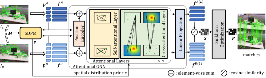
The overview of the proposed matching pipeline is shown in Fig. 2. First, the Spatial Distribution Prior Module (SDPM), which will be presented in detail in Section III-B, computes the spatial distribution prior $\boldsymbol{s}$ by using the keypoints position $\boldsymbol{p}^{A}$, $\boldsymbol{p}^{B}$, and the IMU measurements $\boldsymbol{M}$. Before the attentional GNN layers, the Keypoint Encoder encodes the keypoints position $\boldsymbol{p}$ into feature space $\boldsymbol{f}$. Then, the spatial distribution prior $\boldsymbol{s}$ is fed to the attentional GNN (Section III-C and Section III-D) to assist the keypoint features optimization. Each attentional GNN layer has two types of attention: self-attention and cross-attention. The spatial distribution prior $\boldsymbol{s}$ is integrated into these attention mechanisms in a probabilistic way. Next, the cosine similarity matrix $\boldsymbol{S}$, which is computed by the linear transformed features of the attentional GNN, is optimized by the Sinkhorn algorithm [59] (Section III-E) to obtain the assignment matrix $\boldsymbol{P}$ representing the matching result.

A basic motion assumption is to consider the velocity between two images is constant [29, 30]. To obtain an accurate prior motion, IMU measurements have been widely used in recent SLAM systems to constrain the pose optimization problem [60, 61, 62, 31, 32]. In this paper, we adopt the switched linear system based IMU integration model [31, 32]. It integrates all IMU measurements $\{\boldsymbol{M}_{i}=(\boldsymbol{\omega}_{B},\boldsymbol{a}_{B})_{i}|i\in[1,M]\}$ between $I_{A}$ and $I_{B}$ and outputs motion prior, that is, the initial relative pose $\hat{\boldsymbol{T}}_{AB}$ of $I_{A}$ and $I_{B}$.

As illustrated in Fig. 4, the keypoints prior module first warps the keypoint $\boldsymbol{F}_{i}^{A}=(\boldsymbol{p}_{i},\boldsymbol{f}_{i})^{A}$ in $I_{A}$ to $I_{B}$ with the motion prior $\hat{\boldsymbol{T}}_{AB}$:

where $\Pi(p)$ is the camera projection function that projects a 3D landmark $\boldsymbol{l}\in\mathbb{R}^{3}$ into the camera image plane.

We regard the warped position $\hat{\boldsymbol{p}}_{i}^{A\rightarrow B}$ in $I_{B}$ as keypoint prior knowledge across images. We name it as spatial distribution prior $s_{i,j}$ of keypoints and encode it with Gaussian distribution

where $d_{ij}^{A,B}=\|\hat{\boldsymbol{p}}_{i}^{A\rightarrow B}-\boldsymbol{p}_{j}^{B}\|$ denotes the re-projection distances of keypoint $\hat{\boldsymbol{p}}_{i}^{A\rightarrow B}$ and $\boldsymbol{p}_{j}^{B}$. Similarly, the spatial distribution prior of keypoints in the same image can be obtained with $d_{ij}^{k,k}=\|\boldsymbol{p}_{i}^{k}-\boldsymbol{p}_{j}^{k}\|\ (k\in{A,B})$. In Section III-D, we present two methods to integrate the spatial distribution prior ${\boldsymbol{s}}_{i}$ into attentional GNN.

As shown in Fig. 2, given the features $\boldsymbol{F}^{A}=\{\boldsymbol{p}^{A},\boldsymbol{f}^{A}\}$ and $\boldsymbol{F}^{B}=\{\boldsymbol{p}^{B},\boldsymbol{f}^{B}\}$ of an image pair, we first embed the keypoint position $\boldsymbol{p}$ into its feature space $\boldsymbol{f}$ with the position encoder. This enables the attentional GNN to utilize the position in an implicit way. Following [28], an MLP module is adopted as the position encoder for each feature $\boldsymbol{F}_{i}\in[1,N]$:

The attentional GNN layers for keypoints matching [28] formulates the vertexes as keypoint feature $\boldsymbol{f}$, edges as attention $\alpha$. It optimizes each keypoint feature $\boldsymbol{f}$ iteratively to obtain the contextual information in-and-cross images. Fig. 5 illustrates the process that the $i$-th feature in $I_{A}$ is optimized by all the features in $I_{B}$. In the following, to facilitate the notation, the superscripts $A$ and $B$ are omitted to denote arbitrary keypoint pairs of arbitrary images.

As in transformer [63], the input features are first linear-transformed to the query $\boldsymbol{q}_{i}$, key $\boldsymbol{k}$, and value $\boldsymbol{v}$:

where $j$ denotes the $j$-th feature in images. Then, the attention

is obtained to focus on different values $\boldsymbol{v}$. So that the contextual messages $\textup{m}_{\varepsilon\rightarrow i}$ for the feature $\boldsymbol{f}_{i}$ are propagated through all the edges $\varepsilon\rightarrow i$ connected with vertex $\boldsymbol{f}_{i}$:

The message $\boldsymbol{m}_{\varepsilon\rightarrow i}$ is aggregated into the $i$-th feature $\boldsymbol{f}^{(l-1)}_{i}$ in a residual style. The residual is the MLP dimensionality reduction of the concatenated contextual messages $[\boldsymbol{f}_{i}^{(l-1)}\|\textup{m}_{\varepsilon\rightarrow i}]$:

In the above processes, the self- and cross- attentional GNN layers are used iteratively to imitate the back-and-forth behaviors when asking a human to match keypoints. For a specific feature $\boldsymbol{f}_{i}$ in one image, the self-attention GNN layer propagates contextual messages from the same image, while the cross-attention GNN layer obtains contextual messages from another image. After several self- and cross- attentional GNN layers, the final matching feature $\boldsymbol{f}_{i}$ are linear projections of the last attentional GNN layer outputs $\boldsymbol{f}_{i}^{(L)}$:

It is rational that a keypoint should have strong correlations with the ones close to it. Based on this intuition, the correlation strength of each keypoint should decrease with the distance to others. A straightforward approach to integrating the prior $s_{ij}$ into attentional GNN is using it to weigh the attention in Equation (6). But directly weighting on $\alpha_{ij}$ will break the normalization property, thus we can weigh on the variable of softmax $\alpha_{ij}=\textup{softmax}_{j}(s_{ij}\boldsymbol{q}_{i}^{T}\boldsymbol{k}_{j})$. However, when the distance $d_{ij}$ of feature $i$ and $j$ is greater than $3\sigma$, the prior $s_{ij}$ becomes very close to zero. Thus the attention on other hidden features will be weakened unexpectedly. So the direct spatial prior integration is formulated as

It can be seen that the weight $(1+s_{ij})$ ranges from one to two, so it can preserve the attention on other hidden features even if $s_{ij}=0$. Under this formulation, the spatial prior could hinder the original attention extraction as they are tightly coupled together. So a probabilistic spatial prior integration is proposed to tackle this problem.

To integrate the spatial prior into the attention module in a natural way, we exploit the probabilistic perspective of the attention. In the formulation of the vanilla attention module, i.e. Equation (9), the attention $\alpha_{ij}$ is a normalized Gaussian distribution [64] of the cosine similarity of query $\boldsymbol{q}_{i}$ and key $\boldsymbol{k}_{j}$. With this perspective, the vanilla attention $\alpha_{ij}$ can be regarded as a joint distribution for each embedded features $\boldsymbol{q}_{i}$ and $\boldsymbol{k}_{j}$ as

In fact, it is a distribution conditioned by appearance, spatial characteristics, and other hidden contexts. Our intuition is that the vanilla attention module has to model all the hidden contexts from scratch, which could be difficult. This intuition can be further confirmed with the closer investigations on the attention $\alpha_{ij}$ in each layer. As shown in Fig. 6, the network struggles to find a proper attentional relationship of features across images. With the assistance of spatial distribution prior, the attentional GNN can focus on the modeling of other contexts such as the appearance, and the attentional GNN layers can be streamlined to only two attentional GNN layers, as shown in Fig. 8.

Then, we consider the spatial distribution prior $s_{ij}$ for keypoints $p_{i}$ and $p_{j}$ as a Gaussian distribution

and it is independent of other hidden contexts. As such, with the spatial distribution prior $\Pr(\boldsymbol{f}_{i},\boldsymbol{f}_{j}|\text{spatial})$, the network can be relaxed to solely model the appearance and other hidden contexts $\Pr(\boldsymbol{f}_{i},\boldsymbol{f}_{j}|\text{appearance},...)$. Thus the attentional distribution can be formulated as

With the normalization of the above distribution, this process can be efficiently implemented as

The elements in the assignment matrix $\bar{\boldsymbol{P}}_{1:N_{A},1:N_{B}}$ indicate the matching confidence for each possible keypoint pairs, and the elements in dustbins $\bar{\boldsymbol{P}}_{N_{A}+1,1:N_{B}}$ and $\bar{\boldsymbol{P}}_{1:N_{A},N_{B}+1}$ suggest the unmatched confidence. The direct way to constrain $\bar{\boldsymbol{P}}$ is by using the ground-truth keypoint matching $\mathcal{M}\subseteq\{(i,j)|i\in[1,N_{A}],j\in[1,N_{B}]\}$, unmatching $\mathcal{I}\subseteq[1,N_{A}]$, and $\mathcal{J}\subseteq[1,N_{B}]$.

To obtain the ground-truth matches $\mathcal{M}$, keypoints $\boldsymbol{p}_{i}^{A}$ in the image $I_{A}$ are warped to $I_{B}$ as $\boldsymbol{p}_{i}^{A\rightarrow B}$ with its depth map and ground-truth pose $\boldsymbol{T}_{AB}$. The distance matrix $\mathcal{D}\in\mathbb{R}^{N_{A}\times N_{B}}$ between the warped keypoints $\boldsymbol{p}_{i}^{A\rightarrow B}$ and $\boldsymbol{p}_{j}^{B}$ is computed. Then, the correct matching $\mathcal{M}$ is defined as

where $th$ is a pixel threshold.

As such, the matching loss could be formulated as the mean negative log-likelihood of the assignment $\bar{\boldsymbol{P}}$:

where $\#\mathcal{M}$ denotes the total number of matched keypoint pairs, $\#\mathcal{I}$ and $\#\mathcal{J}$ are the number of unmatched keypoints in $I_{A}$ and $I_{B}$ respectively. Thus the total matching loss is given as

However, in our experiments, we find that the model could not always converge to its best weights with the matching loss. We hypothesize that the hard-threshold ground-truth definition of Equation (16) with a fix $th$ could be sub-optimal. As shown in Fig. 7, the positive matching loss truncates the loss at $th$, regarding all the loss as the same when $d_{ij}<th$, while neglecting the loss for those $d_{ij}>th$.

To address this problem, we relax the threshold $th$ in Equation (16) to a much larger margin $mg$ ($mg>th$), and the loss should be defined with the distance $d_{ij}$. To this end, a subset of $\mathcal{D}$ is defined as positive matches

And the unmatched keypoints $\mathcal{\tilde{I}}$ of $I_{a}$ and $\mathcal{\tilde{J}}$ of $I_{B}$ are those not in the positive matches $\tilde{\mathcal{D}}$.

Under this formulation, each element in $\tilde{\mathcal{D}}$ is a possible match and its value indicates the ground truth matching distance. Then the projection loss of all possible matches is given as

where

The projection loss can constrain the loss of positive samples softer and more reasonably, as shown in Fig. 7. On the one hand, when the matching distance of keypoints is close to zero, they are more likely to be matched. In this case, the loss will push the output confidence to one. On the other hand, a larger ground truth matching distance indicates a weak tie, thus the loss constraint softly decreases with the distance. So that the loss can recall more potential matches.

We compared the proposed method with the handcrafted and learned methods. The proposed method of two attentional GNN layers was trained with projection loss (will be discussed in Section IV-E) for comparisons. For the handcrafted methods, two variations of nearest neighbor (NN) matching, the mutual NN with PyTorch implementation, and the FLANN with OpenCV implementation when the test ratio is 0.7, were evaluated. For the learned methods, the PointCN [16], OANet [18], ACNe [19], and SuperGlue [28] were assessed. During testing, the official released code and model weights were used. Specifically, we used the model trained on GL3D-v2 for OANet [18]. For ACNe [19], the indoor model weights were used, and the keypoint matches with a combined weight is greater than $10^{-7}$ were taken as correct matches. For SuperGlue [28], we assessed the official “indoor” and “outdoor” model weights, as well as the SueprGlue of two attentional GNN layers trained on our training set with the same training configures as for the proposed methods. The matching confidence thresholds of the assignment matrix of SuperGlue and the proposed models were both set to 0.2 as in [28], and we found this configuration gives the best trade-off between precision and recall. All the models were evaluated on a desktop platform with Intel Core i5-4590 and GeForce GTX TITAN X (PASCAL).

The matching results of different learned methods are shown in Fig. 10 and Fig. 11. As can be seen from these figures, the PointNet-like methods generate some false matches (results of PointCN [16] and ACNe [19] in Fig. 10) and obtain fewer matches (results of PointCN [16] and OANet [18] in Fig. 10) than the feature-based models. The possible reason is that the PointNet-like methods only take advantage of the position of keypoints and cannot model the appearance or other hidden features. The full SuperGlue [28] model, on the other hand, achieves the best matching results on the test images. Nevertheless, the full SuperGlue model consumes a lot of computation time (Fig. 11), and is not suitable for real-time SLAM systems. Simplifying SuperGlue by reducing the number of GNN layers can decrease its computational efforts, but it also degrades the matching performance (as shown in Fig. 11). With the assistance of prior information, the proposed method fills this performance decline without increasing the computation time (as shown in Fig. 11).

The ground-truth matches are first obtained according to Equation (16) with $th=3$. Then the matching precision $P_{m}$, recall $R_{m}$, and F1-score is given as

where $TP$, $FP$, and $FN$ denote the true positives, false positives, and false negatives respectively. The $TP$, $TP+FP$, and $TP+FN$ represent the number of correct matches, estimated matches, and ground-truth matches in the keypoints matching case respectively.

The detailed matching results are shown in Table I. It is noticeable that the mNN and FLANN both have good matching precision ($P_{m}$) and recall ($R_{m}$) on our test sets, which is only slightly lower than the SuperGlue [28] and the proposed method. While the PointNet-like models PointCN [16], OANet [18], and ACNe [19] do not perform well on our test sets. This could due to the fact that they follow the putative filtering strategy, so they require massive putative keypoint pairs (usually $>2000$) for each image pair. However, we only extracted the most distinctive keypoints as in most SLAM systems, resulting in fewer keypoints in the image and fewer putative matches in the image pairs. The full SuperGlue [28] model with “outdoor” weights (nine attentional GNN layers) achieves the best matching F1 scores, with an F1 score of 91.40%, 66.15%, and 83.37% on InteriorNet [33], TUM-RGBD [34], and ETH3D [35] respectively. Nonetheless, the SuperGlue of two attentional GNN layers drop the matching performance by 4.57%, 3.36%, and 5.98% for the F1 score on InteriorNet, TUM-RGBD, and ETH3D test sets respectively. The proposed methods, which are assisted by the spatial distribution prior of keypoints, can regain the performance drop of reduction of GNN layers as in Table I. Specifically, the proposed method promotes the recall $R_{m}$ by 4.94%, 7.46%, and 8.05%, F1 scores by 1.27%, 0.53%, and 3.98% on InteriorNet, TUM-RGBD, and ETH3D test sets receptively. Furthermore, as shown in Fig. 12, without the assistance of the spatial distribution prior, SuperGlue of two attentional GNN layers fails to recover correct matches with higher matching confidence (lower F1 score than the proposed method). Some matching examples are shown in Fig. 10.

The purpose of keypoints matching is to estimate the relative pose of two images. So the pose accuracy is also evaluated. Given the predicted keypoint matches of an image pair, the essential matrix is obtained with OpenCV function findEssentialMat, and then the relative pose is recovered with recoverPose. As in previous works [16, 18, 28], we calculate the pose angular differences between ground truth and estimated pose, and report the area under curve (AUC) with a maximum error of threshold 5°, 10°, and 20°.

Five learned models are assessed in Table II. The Pointnet-like models PointCN [16], OANet [18], and ACNe [19] yield lower AUCs. The possible reason is that the number of keypoints is not sufficient for them to recover good matches. The visualization in Fig. 10 suggests they recall fewer matches and produces many false matches. The AUCs of the full SuperGlue [28] model, are generally higher than the PointNet-like models. And the SuperGlue with “indoor” weights obtains the best AUC performance among previously learned methods, yields 38.26%, 19.29%, and 41.04% of AUC@20° on InteriorNet [33], TUM-RGBD [34], and ETH3D [35] test sets respectively. As the SuperGlue of two attentional GNN layers was trained on our training set, it also gives AUCs on par with the full SuperGlue model, with 35.37%, 18.09%, and 39.94% of AUC@20° on InteriorNet, TUM-RGBD, and ETH3D test sets respectively. Due to the assistance of spatial distribution prior, the proposed method produces higher AUCs than SuperGlue of two attentional GNN layers by 3.43%, 1.59%, and 3.29% of AUC@20° on InteriorNet, TUM-RGBD, and ETH3D test sets respectively, and outperforms the other learned methods.

We tested all the learned models with the same agenda to measure the matching time of an image pair. The results are shown in Fig. 13. Among the learned matching networks, the model sizes of ACNe [19], OANet [18], and SuperGlue [28] are larger, which results in longer running times. Since the running time is influenced by the number of points, the larger model in turn amplifies the dispersion of the running time. While the PointCN [16], SuperGlue [28] of two GNN layers and the proposed method have the shortest matching time of about 15 milliseconds. Considering the matching metrics and pose estimation accuracy of the proposed method are much better than those of PointCN [16] and SuperGlue [28] of two GNN layers, the effectiveness of the proposed prior integration and projection loss is verified.

To demonstrate the generalization of the proposed method, experiments are also carried out on homography image pairs. Table III illustrates the matching results of full SuperGlue [28] (with “outdoor” weights), SuperGlue of two attentional GNN layers, and the proposed method. Note that the latter two models were trained only on the RGBD datasets, no homography image pairs are included in the training process. As in Table III, the full SuperGlue [28] with “outdoor” weights achieves the best matching performance, giving F1 scores of 82.52%, 82.73%, and 75.51% on HPatches illumination, viewpoint, and OxfordParis, respectively. However, F1 scores of the two GNN layers version of SuperGlue drops to 60.77%, 51.12%, and 45.58% on these datasets. While the F1 scores of the proposed method significantly outperform the two GNN layers version of SuperGlue, which are 64.73%, 62.18%, and 51.42% respectively. Moreover, as the viewpoint differences on HPatches viewpoint and OxfordParis are larger, the assistance of the spatial distribution prior is more significant. Therefore, the improvement of the F1 score is more obvious, which increases by 10.05% and 5.84% respectively. In addition to the matching performance, the homography estimation accuracy $Acc_{H}$ is also evaluated. The mean reprojection error of the four corners of the image is first computed, and then the homography estimation accuracy is defined by the accuracy of the corner error under a threshold of three pixels. As shown in Table III, the homography accuracy $Acc_{H}$ of the proposed method is slightly lower than SuperGlue [28] on the Hpatches illumination dataset. The proposed method, on the other hand, significantly outperforms SueprGlue of two attentional GNN layers on HPatches viewpoint and OxfordParis datasets. The reason for this phenomenon is that for the Hpatches illumination dataset, the homography matrix is identity, and the noise added during generating the priors interferes with the matching process. For HPatches viewpoint and OxfordParis datasets, there are significant viewpoint differences in a pair of images. Thus the noise is trivial and the prior plays a vital role in improving the matching performance.

The MLP in Equation (3) makes use of position by embedding it to feature space, while the proposed prior integration utilizes the position by propagating contextual keypoint features through the attentional GNN. The two methods of position utilization are compared in this section. As shown in Table IV, the position encoder (penc) promotes the F1 score on the plain network by 0.27%. The proposed direct prior (dprior) and probabilistic prior integration boost the F1 score by 0.9% and 2.7% respectively. The same results can also be found in Fig. 14, where the F1 score is plotted with respect to the matching confidence. It could be because the embedding of positional encoding changes the feature distribution of descriptors, and it is difficult for the network to learn such embedding. While the proposed prior integration does not change the distribution of any features, but only aggregates the nearby features in the original feature space, so the proposed prior integration methods significantly improve the matching performance.

As shown in Table IV, compared to the plain network, after integrating the direct and probabilistic prior into attentional GNN, the precision is improved by 1.77% and 2.58% respectively, and the F1 score is improved 0.9% and 1.7% respectively. With the keypoint position encoder module, the total improvement of the F1 score is 1.08% and 1.79% for the direct and probabilistic prior integration respectively. The same promotion can also be found in Fig. 14. These primary matching results indicate the probabilistic prior integration is more efficient than direct prior integration.

In terms of the accuracy of the estimated pose, inconsistent results are observed for different approaches with the matching results as in Fig. 15. The improvements of AUCs by the direct prior integration are larger than those of probabilistic prior integration, and the improvements of both prior integrations are lower than the positional encoder except that of AUC under 5°. Another interesting result is that the combination of positional encoding and direct prior integration actually deteriorates the pose estimation accuracy. The possible reason could be that the positional embedding feature could not be processed correctly by the direct prior integration strategy. While the combination of positional encoding and probabilistic prior integration can promote each other, and improve the pose accuracy significantly.

We evaluated the matching loss of Equation (17) and the projection loss of Equation (21) by training the plain network (with two attentional GNN layers and an optimization layer) on the same train dataset with a fixed random seed. As expected, the projection loss recalls more matches than matching loss due to its relaxation of the matching threshold, thus yields higher $F1$ scores as shown in Fig. 16. Thus, we use the projection loss for all experiments.

Since the introduction of the spatial distribution prior can assist the model to utilize the contextual features, so that the number of attentional GNN layers is reduced for efficiency. To verify the impact of the number of GNN layers on the performance, we trained and assessed the models of one to five attention GNN layers. The matching results are shown in Fig. 16. Clearly, the model with more GNN layers has a better matching performance. However, when the number of GNN layers is larger than one, there is no significant performance improvement, but the running time is greatly increased. As shown in Table V, the pose estimation accuracy even decreases with the increase of the number of GNN layers, as a deeper model is harder to train. To balance the performance and efficiency, we use two attentional GNN layers.

References

- [1] C. G. Harris and M. Stephens, “A combined corner and edge detector.” in Alvey vision conference, vol. 15. Citeseer, 1988, pp. 10–5244.
- [2] J. Shi, “Good features to track,” in 1994 Proceedings of IEEE conference on computer vision and pattern recognition. IEEE, 1994, pp. 593–600.
- [3] S. Alkaabi and F. Deravi, “Candidate pruning for fast corner detection,” Electronics Letters, vol. 40, no. 1, pp. 18–19, 2004.
- [4] A. Barroso-Laguna, E. Riba, D. Ponsa, and K. Mikolajczyk, “Key. net: Keypoint detection by handcrafted and learned cnn filters,” in Proceedings of the IEEE International Conference on Computer Vision, 2019, pp. 5836–5844.
- [5] R. Hartley and A. Zisserman, Multiple view geometry in computer vision. Cambridge university press, 2003.
- [6] C. Ding and Z. Ma, “Multi-Camera Color Correction via Hybrid Histogram Matching,” IEEE Transactions on Circuits and Systems for Video Technology, Dec. 2020, doi: 10.1109/TCSVT.2020.3038484.
- [7] Q. Wang, W. Chen, X. Wu, and Z. Li, “Detail-enhanced multi-scale exposure fusion in YUV color space,” IEEE Transactions on Circuits and Systems for Video Technology, vol. 30, no. 8, pp. 2418–2429, Aug. 2020.
- [8] C. Zheng, Z. Li, Y. Yang, and S. Wu, “Single Image Brightening via Multi-Scale Exposure Fusion with Hybrid Learning,” IEEE Transactions on Circuits and Systems for Video Technology, Jun. 2020, doi: 10.1109/TCSVT.2020.3009235.
- [9] J. Ma, J. Zhao, J. Jiang, H. Zhou, and X. Guo, “Locality Preserving Matching,” International Journal of Computer Vision, vol. 127, no. 5, pp. 512–531, May 2019.
- [10] D. G. Lowe, “Distinctive image features from scale-invariant keypoints,” International journal of computer vision, vol. 60, no. 2, pp. 91–110, 2004.
- [11] O. Pele and M. Werman, “A linear time histogram metric for improved sift matching,” in European conference on computer vision. Springer, 2008, pp. 495–508.
- [12] X. Li and Z. Hu, “Rejecting mismatches by correspondence function,” International Journal of Computer Vision, vol. 89, no. 1, pp. 1–17, 2010.
- [13] Y. Lipman, S. Yagev, R. Poranne, D. W. Jacobs, and R. Basri, “Feature matching with bounded distortion,” ACM Transactions on Graphics (TOG), vol. 33, no. 3, pp. 1–14, 2014.
- [14] J. Ma, J. Zhao, J. Tian, A. L. Yuille, and Z. Tu, “Robust Point Matching via Vector Field Consensus,” IEEE Transactions on Image Processing, vol. 23, no. 4, pp. 1706–1721, Apr. 2014.
- [15] W.-Y. Lin, F. Wang, M.-M. Cheng, S.-K. Yeung, P. H. Torr, M. N. Do, and J. Lu, “CODE: Coherence based decision boundaries for feature correspondence,” IEEE transactions on pattern analysis and machine intelligence, vol. 40, no. 1, pp. 34–47, 2017.
- [16] K. M. Yi, E. Trulls, Y. Ono, V. Lepetit, M. Salzmann, and P. Fua, “Learning to Find Good Correspondences,” in 2018 IEEE/CVF Conference on Computer Vision and Pattern Recognition. Salt Lake City, UT, USA: IEEE, Jun. 2018, pp. 2666–2674.
- [17] C. Zhao, Z. Cao, C. Li, X. Li, and J. Yang, “NM-Net: Mining Reliable Neighbors for Robust Feature Correspondences,” in Proceedings of the IEEE Conference on Computer Vision and Pattern Recognition, 2018.
- [18] J. Zhang, D. Sun, Z. Luo, A. Yao, L. Zhou, T. Shen, Y. Chen, H. Liao, and L. Quan, “Learning Two-View Correspondences and Geometry Using Order-Aware Network,” in 2019 IEEE/CVF International Conference on Computer Vision (ICCV). Seoul, Korea (South): IEEE, Oct. 2019, pp. 5844–5853.
- [19] W. Sun, W. Jiang, E. Trulls, A. Tagliasacchi, and K. M. Yi, “ACNe: Attentive Context Normalization for Robust Permutation-Equivariant Learning,” in Proceedings of the IEEE/CVF Conference on Computer Vision and Pattern Recognition, 2020, pp. 11 286–11 295.
- [20] H. Bay, T. Tuytelaars, and L. Van Gool, “Surf: Speeded up robust features,” in European conference on computer vision. Springer, 2006, pp. 404–417.
- [21] K. M. Yi, E. Trulls, V. Lepetit, and P. Fua, “LIFT: Learned Invariant Feature Transform,” in European Conference on Computer Vision, vol. 9910. Cham: Springer, 2016, pp. 467–483.
- [22] X. Han, T. Leung, Y. Jia, R. Sukthankar, and A. C. Berg, “Matchnet: Unifying feature and metric learning for patch-based matching,” in Proceedings of the IEEE Conference on Computer Vision and Pattern Recognition, 2015, pp. 3279–3286.
- [23] A. Mishchuk, D. Mishkin, F. Radenovic, and J. Matas, “Working hard to know your neighbor’s margins: Local descriptor learning loss,” in Advances in Neural Information Processing Systems, Jan. 2018.
- [24] Y. Tian, X. Yu, B. Fan, F. Wu, H. Heijnen, and V. Balntas, “SOSNet: Second Order Similarity Regularization for Local Descriptor Learning,” in Conference on Computer Vision and Pattern Recognition, Dec. 2019.
- [25] D. DeTone, T. Malisiewicz, and A. Rabinovich, “SuperPoint: Self-Supervised Interest Point Detection and Description,” in Proceedings of the IEEE Conference on Computer Vision and Pattern Recognition Workshops, 2018, pp. 224–236.
- [26] M. Dusmanu, I. Rocco, T. Pajdla, M. Pollefeys, J. Sivic, A. Torii, and T. Sattler, “D2-Net: A Trainable CNN for Joint Description and Detection of Local Features,” in 2019 IEEE/CVF Conference on Computer Vision and Pattern Recognition (CVPR). Long Beach, CA, USA: IEEE, Jun. 2019, pp. 8084–8093.
- [27] J. Revaud, P. Weinzaepfel, C. D. Souza, N. Pion, G. Csurka, Y. Cabon, and M. Humenberger, “R2D2: Repeatable and Reliable Detector and Descriptor,” in NeurIPS, 2019, p. 12.
- [28] P.-E. Sarlin, D. DeTone, T. Malisiewicz, and A. Rabinovich, “SuperGlue: Learning Feature Matching with Graph Neural Networks,” in Proceedings of the IEEE/CVF Conference on Computer Vision and Pattern Recognition, Mar. 2020, pp. 4938–4947.
- [29] R. Mur-Artal and J. D. Tardós, “ORB-SLAM2: An open-source slam system for monocular, stereo, and rgb-d cameras,” IEEE Transactions on Robotics, vol. 33, no. 5, pp. 1255–1262, 2017.
- [30] J. Zhang and S. Singh, “LOAM: Lidar Odometry and Mapping in Real-time.” Robotics: Science and Systems Foundation, Jul. 2014.
- [31] J. Henawy, Z. Li, W. Y. Yau, G. Seet, and K. W. Wan, “Accurate IMU Preintegration Using Switched Linear Systems For Autonomous Systems,” in 2019 IEEE Intelligent Transportation Systems Conference (ITSC). Auckland, New Zealand: IEEE, Oct. 2019, pp. 3839–3844.
- [32] J. Henawy, Z. Li, W. Y. Yau, and G. Seet, “Accurate IMU Factor Using Switched Linear Systems For VIO,” IEEE Transactions on Industrial Electronics, vol. 68, no. 9, pp. 1–10, Sep. 2021.
- [33] W. Li, S. Saeedi, J. McCormac, R. Clark, D. Tzoumanikas, Q. Ye, Y. Huang, R. Tang, and S. Leutenegger, “InteriorNet: Mega-scale Multi-sensor Photo-realistic Indoor Scenes Dataset,” in British Machine Vision Conference (BMVC), 2018.
- [34] J. Sturm, N. Engelhard, F. Endres, W. Burgard, and D. Cremers, “A benchmark for the evaluation of RGB-D SLAM systems,” in 2012 IEEE/RSJ International Conference on Intelligent Robots and Systems, Oct. 2012, pp. 573–580.
- [35] T. Schops, T. Sattler, and M. Pollefeys, “BAD SLAM: Bundle Adjusted Direct RGB-D SLAM,” in 2019 IEEE/CVF Conference on Computer Vision and Pattern Recognition (CVPR). Long Beach, CA, USA: IEEE, Jun. 2019, pp. 134–144.
- [36] E. Rublee, V. Rabaud, K. Konolige, and G. Bradski, “ORB: An efficient alternative to SIFT or SURF,” in 2011 International conference on computer vision. Ieee, 2011, pp. 2564–2571.
- [37] V. Balntas, E. Riba, D. Ponsa, and K. Mikolajczyk, “Learning local feature descriptors with triplets and shallow convolutional neural networks.” in BMVC, vol. 1, 2016, p. 3.
- [38] Y. Tian, B. Fan, and F. Wu, “L2-Net: Deep Learning of Discriminative Patch Descriptor in Euclidean Space,” in 2017 IEEE Conference on Computer Vision and Pattern Recognition. Honolulu, HI: IEEE, Jul. 2017, pp. 6128–6136.
- [39] Y. Ono, E. Trulls, P. Fua, and K. M. Yi, “LF-Net: Learning Local Features from Images,” in Advances in Neural Information Processing Systems 31. Curran Associates, Inc., 2018, pp. 6234–6244.
- [40] Y. Verdie, K. Yi, P. Fua, and V. Lepetit, “Tilde: A temporally invariant learned detector,” in Proceedings of the IEEE Conference on Computer Vision and Pattern Recognition, 2015, pp. 5279–5288.
- [41] N. Savinov, A. Seki, L. Ladicky, T. Sattler, and M. Pollefeys, “Quad-networks: unsupervised learning to rank for interest point detection,” in Proceedings of the IEEE conference on computer vision and pattern recognition, 2017, pp. 1822–1830.
- [42] X. Guo and X. Cao, “Good match exploration using triangle constraint,” Pattern Recognition Letters, vol. 33, no. 7, pp. 872–881, 2012.
- [43] J. Ma, J. Jiang, H. Zhou, J. Zhao, and X. Guo, “Guided locality preserving feature matching for remote sensing image registration,” IEEE transactions on geoscience and remote sensing, vol. 56, no. 8, pp. 4435–4447, 2018.
- [44] J. Bian, W.-Y. Lin, Y. Matsushita, S.-K. Yeung, T.-D. Nguyen, and M.-M. Cheng, “Gms: Grid-based motion statistics for fast, ultra-robust feature correspondence,” in Proceedings of the IEEE Conference on Computer Vision and Pattern Recognition, 2017, pp. 4181–4190.
- [45] Y.-T. Hu, Y.-Y. Lin, H.-Y. Chen, K.-J. Hsu, and B.-Y. Chen, “Matching images with multiple descriptors: An unsupervised approach for locally adaptive descriptor selection,” IEEE Transactions on Image Processing, vol. 24, no. 12, pp. 5995–6010, 2015.
- [46] J. Maier, M. Humenberger, M. Murschitz, O. Zendel, and M. Vincze, “Guided matching based on statistical optical flow for fast and robust correspondence analysis,” in European Conference on Computer Vision. Springer, 2016, pp. 101–117.
- [47] Y. Liu, L. De Dominicis, B. Wei, L. Chen, and R. R. Martin, “Regularization based iterative point match weighting for accurate rigid transformation estimation,” IEEE transactions on visualization and computer graphics, vol. 21, no. 9, pp. 1058–1071, 2015.
- [48] L. Torresani, V. Kolmogorov, and C. Rother, “Feature Correspondence via Graph Matching: Models and Global Optimization,” in European Conference on Computer Vision, 2008.
- [49] S. Liu, H. Wang, Y. Wei, and C. Pan, “Bb-homography: Joint binary features and bipartite graph matching for homography estimation,” IEEE Transactions on Circuits and Systems for Video Technology, vol. 25, no. 2, pp. 239–250, 2015.
- [50] R. Zhang and W. Wang, “Second- and high-order graph matching for correspondence problems,” IEEE Transactions on Circuits and Systems for Video Technology, vol. 28, no. 10, pp. 2978–2992, 2018.
- [51] Y. F. Yu, G. Xu, K. K. Huang, H. Zhu, L. Chen, and H. Wang, “Dual calibration mechanism based l2,p-norm for graph matching,” IEEE Transactions on Circuits and Systems for Video Technology, 2020, doi:10.1109/TCSVT.2020.3023781.
- [52] M. A. Fischler and R. C. Bolles, “Random sample consensus: a paradigm for model fitting with applications to image analysis and automated cartography,” Communications of the ACM, vol. 24, no. 6, pp. 381–395, 1981.
- [53] N. Ufer and B. Ommer, “Deep semantic feature matching,” in Proceedings of the IEEE Conference on Computer Vision and Pattern Recognition, 2017, pp. 6914–6923.
- [54] W. Yu, X. Sun, K. Yang, Y. Rui, and H. Yao, “Hierarchical semantic image matching using CNN feature pyramid,” Computer Vision and Image Understanding, vol. 169, pp. 40–51, 2018.
- [55] S. Khan, M. Nawaz, X. Guoxia, and H. Yan, “Image correspondence with cur decomposition-based graph completion and matching,” IEEE Transactions on Circuits and Systems for Video Technology, vol. 30, no. 9, pp. 3054–3067, 2020.
- [56] F. Kou, Z. Li, C. Wen, and W. Chen, “Multi-scale exposure fusion via gradient domain guided image filtering,” in 2017 IEEE International Conference on Multimedia and Expo (ICME), 2017, pp. 1105–1110.
- [57] J. Zheng, Z. Li, Z. Zhu, S. Wu, and S. Rahardja, “Hybrid patching for a sequence of differently exposed images with moving objects,” IEEE Transactions on Image Processing, vol. 22, no. 12, pp. 5190–5201, 2013.
- [58] C. R. Qi, H. Su, K. Mo, and L. J. Guibas, “PointNet: Deep Learning on Point Sets for 3D Classification and Segmentation,” in Proceedings of the IEEE conference on computer vision and pattern recognition, 2017, pp. 652–660.
- [59] M. Cuturi, “Sinkhorn Distances: Lightspeed Computation of Optimal Transport,” in Advances in Neural Information Processing Systems 26. Curran Associates, Inc., 2013, pp. 2292–2300.
- [60] R. Mur-Artal and J. D. Tardós, “Visual-inertial monocular SLAM with map reuse,” IEEE Robotics and Automation Letters, vol. 2, no. 2, pp. 796–803, 2017.
- [61] T. Qin, P. Li, and S. Shen, “VINS-Mono: A Robust and Versatile Monocular Visual-Inertial State Estimator,” IEEE Transactions on Robotics, vol. 34, no. 4, pp. 1004–1020, Aug. 2018.
- [62] C. Forster, L. Carlone, F. Dellaert, and D. Scaramuzza, “On-Manifold Preintegration for Real-Time Visual–Inertial Odometry,” IEEE Transactions on Robotics, vol. 33, no. 1, pp. 1–21, 2017.
- [63] A. Vaswani, N. Shazeer, N. Parmar, J. Uszkoreit, L. Jones, A. N. Gomez, L. Kaiser, and I. Polosukhin, “Attention is All you Need,” in Advances in Neural Information Processing Systems 30. Curran Associates, Inc., 2017, pp. 5998–6008.
- [64] X. Wang, R. Girshick, A. Gupta, and K. He, “Non-local neural networks,” in Proceedings of the IEEE conference on computer vision and pattern recognition, 2018, pp. 7794–7803.
- [65] G. Peyré and M. Cuturi, “Computational Optimal Transport,” arXiv:1803.00567 [stat], Mar. 2020.
- [66] J. Munkres, “Algorithms for the assignment and transportation problems,” Journal of the society for industrial and applied mathematics, vol. 5, no. 1, pp. 32–38, 1957.
- [67] V. Balntas, K. Lenc, A. Vedaldi, and K. Mikolajczyk, “HPatches: A benchmark and evaluation of handcrafted and learned local descriptors,” in Proceedings of the IEEE Conference on Computer Vision and Pattern Recognition, 2017, pp. 5173–5182.
- [68] F. Radenović, A. Iscen, G. Tolias, Y. Avrithis, and O. Chum, “Revisiting oxford and paris: Large-scale image retrieval benchmarking,” in Proceedings of the IEEE Conference on Computer Vision and Pattern Recognition, 2018, pp. 5706–5715.
- [69] D. P. Kingma and J. Ba, “Adam: A Method for Stochastic Optimization,” in ICLR, 2015.