Let us begin by considering the fibres of $\alpha(x,y)=x$ in $A$, which correspond to radial lines. These fibres necessarily intersect their images as a consequence of the twist condition and the intermediate value theorem, as can be seen in Figure 5.

Next, isolate the intersections of these fibres with their images as in Figure 6(a). One can imagine that if we were to run this process for progressively denser sets of fibres of $\alpha$, we might hope to obtain a set of smooth curves. These curves would be $x-$invariant in the sense that they satisfy the equation $f_{1}(x,y)=x$ (i.e., the $x-$coordinate of the points in these curves is unchanged by $f$).

The intersection points in Figure 6(b) must exist because otherwise the region enclosed by some $x-$invariant curve would necessarily be mapped to a proper subset or superset of itself, which contradicts the assumption that $f$ admits a positive integral invariant. Then one might conclude that these intersection points are fixed points. However, there are two claims here needing further justification:

1. 1.

   The invariant curves exist.

2. 2.

   The intersection points of invariant curves and their images constitute fixed points of $f$.

It turns out (1) is indeed provable, however (2) is not necessarily true. Thus, the proof will proceed as a variation of the intuitive approach outlined here.

Proving the existence of the hinted at $x-$invariant curves is nearly a direct application of the preimage theorem to the map

In which case $F^{-1}(0)$ would be composed of the desired set of invariant curves.

However, it cannot be guaranteed that $0$ is a regular value of our $F$, a necessary condition for the application of the preimage theorem. Thus, we need a slightly stronger result, the parametric transversality theorem.

To apply Theorem 4.2 we parameterize $\alpha$ by an additional parameter, $\phi\in\mathbb{R}_{+}$, by $\alpha_{\phi}(x,y)=\phi\cdot x-y$. This naturally implies a redefinition of $F:\mathbb{R}_{+}\times A\rightarrow\mathbb{R}$, given now by

When we wish $\phi$ to be held constant, we denote $F(\phi,x,y)$ by $F_{\phi}(x,y)$.

Now we need to show $0$ is a regular value of $F$. In particular, we need to show that

is onto for all $(x,y)\in F^{-1}(0)$. If $DF$ weren’t onto, then each of its entries must be equal to $0$, which would imply $x=f_{1}$. This along with $F_{\phi}(x,y)=0$ would tell us $f(x,y)=(x,y)$. That is, $DF$ can only fail to be onto if $(x,y)$ is a fixed point of $f$.

Thus, there are exactly two possibilities:

1. 1.

   There is a set of $\phi$ of full measure such that $F_{\phi}$ is transverse to $0$.

2. 2.

   There is a fixed point of $f$ in $A$.

After covering several additional preliminary results, we begin the central thrust of the proof of Theorem 2.1 in Section 5. There we show that (1) contradicts the existence of a positive integral invariant, thus establishing that $f$ has at least one fixed point in $A$. Then in Section 6 we show that the assumption in (2) of a unique fixed point also leads to a contradiction. In fact, by a slight modification of the previous argument the assumption of a unique fixed point still contradicts the existence of a positive integral invariant.

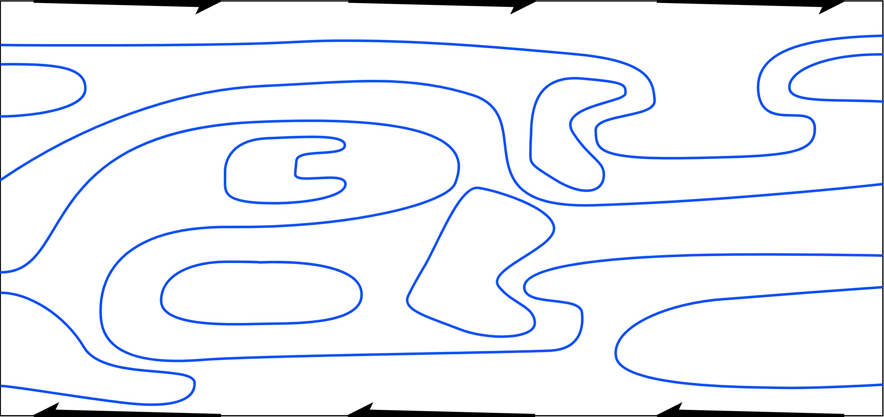
If (1) holds, then, by the definition of transversality, there exists $\phi\in\mathbb{R}_{+}$ such that $0$ is a regular value of $F_{\phi}$. So, by the preimage theorem, $F^{-1}_{\phi}(0)$ is a compact $1-$dimensional submanifold of $A$ and thus contains a finite number of connected components (all closed curves, by the classification of compact $1-$manifolds). Give each component the preimage orientation. This choice of orientation endows each component which wraps around the annulus with winding number $\pm 1$ and all other components with winding number $0$. Figure 7 provides an example of the sort of geometry we might expect here. When there is no risk of ambiguity, $F^{-1}_{\phi}(0)$ is referred to as $\mathcal{I}_{\phi}$ or simply as $\mathcal{I}$.

The parameterization of $\alpha$ with respect to $\phi$, necessary to apply Theorem 4.2 and the preimage theorem, complicates things slightly by endowing $\alpha_{\phi}(x,y)=\phi\cdot x-y$ with slanted fibres in comparison to the straight fibres of the original $\alpha(x,y)=x$. So, to simplify the analysis, we conjugate the system by the linear transformation

with inverse

In these coordinates, the fibres of $\alpha$ are straight, so $f$ translates $\mathcal{I}$ vertically (viewing $A$ as the $1$-periodic strip). Moreover, conjugation by $T$ is simply a change of coordinates, so the hypotheses of the theorem remain satisfied.

Let $\gamma:[0,1]\rightarrow\mathbb{R}^{2}$ be a parameterization of a simple closed curve. Then the winding number of $\gamma$ about $z\in\mathbb{R}^{2}$ is given by

where $\deg(g)$ is the topological degree of $g$.

Note that if any component $S\subseteq\mathcal{I}$ with $W(S)=\pm 1$ is free of non-degenerate critical points (see definition below), then the region bounded by $S$ violates the existence of a positive integral invariant. Thus, for the remainder of this section, we will operate under the assumption that such non-degenerate critical points exist for each $S\subseteq\mathcal{I}$ (such non-degenerate critical points trivially exist for $S$ with $W(S)=0$). Here, we view $A$ as the $1-$periodic strip $(\mathbb{R}/\mathbb{Z})\times[0,1]$, as in Figure 7, rather than the geometric annulus, as in Figure 5. Also let $\pi(x,y)=x$. As usual we define the $\epsilon-$neighborhood of a set $X\subseteq A$ as $\{(x,y)\in A:\inf\limits_{(x^{\prime},y^{\prime})\in X}|(x,y)-(x^{\prime},y^{\prime})|<\epsilon\}$.

• •

  A point $(x_{0},y_{0})\in S\subseteq\mathcal{I}$ is a critical point if $\dfrac{\partial F_{\phi}}{\partial y}(x_{0},y_{0})=0$ (here $S$ is the component of $\mathcal{I}$ containing $(x_{0},y_{0})$). In other words, the tangent to $S$ at $(x_{0},y_{0})$ is vertical.

• •

  A critical point $(x_{0},y_{0})\in S\subseteq\mathcal{I}$ is non-degenerate if there exists $\epsilon>0$ such that the $\epsilon-$neighborhood $U$ of $S\cap(\{x_{0}\}\times(0,1))$ satisfies $\pi(U\cap S)\leq x_{0}$ or $\pi(U\cap S)\geq x_{0}$. Intuitively, $(x_{0},y_{0})$ is non-degenerate if the vertical line $x_{0}\times(0,1)$ does not locally cross $S$.

• •

  A non-degenerate critical point is left-facing (respectively, right-facing) if its tangent is locally to its left (respectively, right). Each of the non-degenerate critical points in Figure 9 are left-facing.

• •

  The outer flow at a non-degenerate critical point is the direction of the $x-$component of the vector field $f(x,y)-(x,y)$ on the vertical tangent near said critical point.

What follows is a set of conventions which will be used to represent and algebraically manipulate the properties of the $S_{i}$ and the non-degenerate critical points.

• •

  Enumerate the $n$ connected components of $\mathcal{I}$ as $\{S_{i}\}_{i=1}^{n}$.

• •

  For each $S_{i}$, define the following:

  • –

    $u_{i}$ is the (constant) sign of $f_{2}(x,y)-y$ in $S_{i}$, denoting the vertical translation direction of $S_{i}$ under $f$.

  • –

    $n_{i}$ is the number of non-degenerate critical points of $S_{i}$.

  • –

    $\{c_{i,k}\}_{k=1}^{n_{i}}$ is the set of non-degenerate critical points of $S_{i}$, each equipped with a value:

    • *

      $c_{i,k}=+1$ if the non-degenerate critical point is right-facing,

    • *

      $c_{i,k}=-1$ if the non-degenerate critical point is left-facing.

  • –

    For $c_{i,k}$, define a corresponding $f_{i,k}$, denoting the direction of the outer flow at $c_{i,k}$:

    • *

      $f_{i,k}=+1$ if the outer flow at $c_{i,k}$ is to the right,

    • *

      $f_{i,k}=-1$ if the outer flow at $c_{i,k}$ is to the left.

  • –

    For $c_{i,k}$, define $T(c_{i,k})=u_{i}c_{i,k}$, called the “type” of $c_{i,k}$.

Now we can begin constructing the closed curve $C$. For each non-degenerate critical point $c_{i,k}$ of type $+1$ (that is, with $T(c_{i,k})=u_{i}c_{i,k}=1$) we define a directed path departing from it as follows.

1. 1.

   Begin traveling vertically in the $v=-f_{i,k}$ direction (i.e., $v=+1$ means up and $v=-1$ means down).

2. 2.

   Once another component $S_{i^{\prime}}$ of $\mathcal{I}$ is intersected, travel along it in the $t=-u_{i^{\prime}}vf_{i,k}$ direction (i.e., right if $t=+1$ and left if $t=-1$) until another non-degenerate critical point $c_{i^{\prime},k^{\prime}}$ is reached.

Adjacent non-degenerate critical points alternate in direction. Thus, because each component of $\mathcal{I}$ has at least one non-degenerate critical point, we can conclude that each component has at least one non-degenerate critical point of type $+1$. Then, since $\mathcal{I}$ is a compact 1-manifold, Lemma 5.1 directly implies there is a finite and non-zero number of non-degenerate critical points of type $+1$.

Note that this is not the same as requiring that $C$ and $f(C)$ have an empty intersection. We only require that $f(C)$ lies entirely within the closure of one of the two connected components of $A\setminus C$.

The remainder of this section is focused on the proof of Lemma 5.1 and Lemma 5.2.

Let $c_{i,k}$ be an arbitrary non-degenerate critical point on $S_{i}\subseteq A$ with $T(c_{i,k})=+1$. The proof of Lemma 5.1 can be reduced to three facts.

1. 1.

   The vertical path taken from $c_{i,k}$ (as defined above Lemma 5.1) intersects another component $S_{i^{\prime}}\subseteq\mathcal{I}$ and, in particular, does not intersect $\partial A$.

2. 2.

   Once $S_{i^{\prime}}$ is hit, the continuation along $S_{i^{\prime}}$ eventually reaches another non-degenerate critical point $c_{i^{\prime},k^{\prime}}$.

3. 3.

   The terminal non-degenerate critical point $c_{i^{\prime},k^{\prime}}$ is of type $+1$.

To prove Lemma 5.2, it will be sufficient to show that the path does not cross over its image.

We prove the existence of this lower bound in two steps: (1) We show that the closed loop from Lemma 5.2 has non-zero winding number, and (2) we use this fact to construct such a lower bound.

By the compactness of $A$ and the continuity of $Df$, the extreme value theorem guarantees there exists $M<\infty$ such that $M\leq|\det(Df(x))|$ for all $x\in A$.

Thus, the area deviation resulting from errors within $B_{\epsilon}(x^{\ast})$ is bounded by $\mu(B_{\epsilon}(x^{\ast}))\sup_{x\in B_{\epsilon}(x^{\ast})}|\det(Df)|$, which is bounded from above by $\mu(B_{\epsilon}(x^{\ast}))M$. Moreover, we have $\mu(B_{\epsilon}(x^{\ast}))\to 0$ as $\epsilon\to 0$, so we can choose $\epsilon>0$ sufficiently small in order to get

which implies

This contradicts the existence of an integral invariant, so we can conclude $f$ has at least two fixed points.

References

- [1] Bramham Barney, Poincaré’s Last Geometric Theorem: A 21st Century Proof, Institut Henri Poincaré, 2013.
- [2] George D. Birkhoff, Proof of Poincaré’s Geometric Theorem, Transactions of the American Mathematical Society 14 (1913), no. 1, 14–22.
- [3] George D. Birkhoff, An Extension of Poincaré’s Last Geometric Theorem, Acta Math. 47 (1926), no. 4, 297–311.
- [4] Christophe Golé and Glen R. Hall, Poincaré’s Proof of Poincaré’s Last Geometric Theorem, Twist Mappings and Their Applications 44 (1992), 135–152.
- [5] Victor Guillemin and Alan Pollack, Differential Topology, AMS Chelsea Publishing, 1974.
- [6] John Hubbard and Yulij Ilyashenko, A Proof of Kolmogorov’s Theorem, Discrete and Continuous Dynamical Systems 4 (2003), no. 4, 1–20.
- [7] Encyclopedia of Mathematics, Poincaré Theorem, http://encyclopediaofmath.org/index.php?title=Poincar%C3%A9_theorem&oldid=48210m.
- [8] Henri Poincaré, Sur un Théoréme de Géométrie, Rendiconti del Circolo Matematico di Palermo 33 (1912), 375–407.
Resumen: Mostramos que el teorema de punto fijo de Poincaré-Birkhoff puede ser probado vía una extensión del acercamiento geométrico originalmente divisado por el propio Poincaré, junto con algunos resultados elementales de topología diferencial. Tras un ejemplo de aplicación del teorema, procedemos a sistemáticamente construir y clasificar cierto conjunto de curvas invariantes y sus puntos críticos. Esta clasificación es luego utilizada para probar la corrección de un procedimiento que garantiza la existencia de por lo menos dos puntos fijos de cualquier función twist de un anillo siempre que admita una integral invariante positiva.
Palabras clave: Dinámica, topología diferencial, problema restringido de los tres cuerpos.
Andrew Graven
Department of Mathematics,
Cornell University
301 Tower Rd,
Ithaca, NY 14853
United States
ajg362@cornell.edu, andrew@graven.com
John Hubbard
jhh8@cornell.edu