跳到论文正文
W Papers独立论文阅读器 arXiv:2111.08734 论文正文 计算阅读时间 · 0%
引用这篇论文根据当前论文元数据生成,正式投稿前建议核对。


License: arXiv.org perpetual non-exclusive license
arXiv:2111.08734v2 [eess.SY] 12 Aug 2022

Formal Synthesis of Controllers for Uncertain Linear Systems against ω\omega-Regular Properties: A Set-based Approach

Bingzhuo Zhong1 , Majid Zamani2,3 and Marco Caccamo1 Address: 1TUM School of Engineering and Design, Technical University of Munich, Germany Email address: {bingzhuo.zhong,mcaccamo}@tum.de Address: 2Department of Computer Science, University of Colorado Boulder, USA Address: 3Department of Computer Science, LMU Munich, Germany Email address: majid.zamani@colorado.edu
Abstract.

In this paper, we present how to synthesize controllers to enforce ω\omega-regular properties over linear control systems affected by bounded disturbances. In particular, these controllers are synthesized based on so-called hybrid controlled invariant (HCI) sets. To compute these sets, we first construct a product system between the linear control system and the deterministic Streett automata (DSA) modeling the desired property. Then, we compute the maximal HCI set over the state set of the product system by leveraging a set-based approach. To ensure termination of the computation of the HCI sets within a finite number of iterations, we also propose two iterative schemes to compute approximations of the maximal HCI set. Finally, we show the effectiveness of our results via two case studies.

1. Introduction

Formal synthesis of control systems has received significant attention in the past few years [1] due to increasing demand for correct-by-construction controllers in many safety-critical real-life applications, such as autonomous vehicles and unmanned aerial vehicles. These synthesis problems become more challenging when handling high-level logic properties, e.g. those expressed as linear temporal logic (LTL) formulae [2], which are widely employed to specify properties for many applications, including [3, 4]. In this paper, we focus on designing controllers enforcing ω\omega-regular properties [5], which is a superset of LTL properties, over discrete-time linear control systems affected by bounded disturbances.

1.1. Related Works

In the computer science community, reactive synthesis [6] was introduced to synthesize controllers enforcing high-level logical properties, see e.g. [6, 7, 8]. However, these results are only applicable to systems with finite state and input sets. As for systems with continuous state and input sets, Hamilton-Jacobi-based (HJ-based) methods [9, 10] are applicable to synthesize controllers against invariance and reachability properties. However, it is challenging to apply these methods to enforce high-level logic properties, in general. To cope with high-level logic properties, discretization-based approaches have been proposed in the past two decades. Among them, symbolic techniques (see e.g. [11, 12, 13]) are widely applied for various types of properties, such as (safe-)LTL (see e.g. [14, 15]) and ω\omega-regular properties (see e.g. [16, 17]). These techniques require the construction of symbolic models (a.k.a. finite abstractions) with finite state and input sets for the original systems. Since the finite state and input sets are constructed by gridding the original sets, the number of discrete states and inputs grow exponentially with respect to the dimensions of state and input sets, respectively. This issue is known as the curse of dimensionality, which is one of the main challenges of discretization-based approaches. Some recent results alleviate this issue partially by constructing abstractions in a compositional manner (see e.g. [18, 19, 20]), by leveraging a counterexample-guided abstraction refinement framework [21], or by applying a specification-guided framework (see e.g. [22, 23, 24]). However, these results require either specific properties of the systems (e.g. dissipativity, mixed-monotonicity, etc.), or additional assumptions regarding the properties (e.g. properties can be decomposed into several simpler ones).

Recently, other discretization-based approaches, which are developed based on interval analysis (referred to as interval-analysis-based approaches), have been proposed to enforce invariance properties [25], reach-and-stay properties [26], and properties modeled by deterministic Büchi automaton [27], which are subsets of ω\omega-regular properties. Despite improvements in terms of space complexity compared with the symbolic techniques, interval-analysis-based approaches also suffer from the curse of dimensionality, since discretization of the state sets is still needed. Additionally, they are only applicable to systems without exogenous disturbances.

To avoid the curse of dimensionality introduced by discretizing the state and input sets, some discretization-free approaches have been proposed. Results in [28] propose a set-based approach to enforce invariance properties (i.e. the systems are expected to stay within a set). This result is further extended in [29, 30, 31, 32] in terms of termination and compositionality. Control barrier functions (CBF) [33] are also used to enforce invariance properties (e.g. [34, 35, 36, 37]), properties described by deterministic finite automata [38, 39], deterministic Büchi automata [40], LTL [41], and ω\omega-regular properties [42]. Unfortunately, constructing valid CBFs is an NP-hard problem in general [43].

1.2. Contribution

In this paper, we propose new discretization-free approaches for synthesizing controllers against ω\omega-regular properties over discrete-time linear control systems affected by bounded disturbances. Concretely, we develop set-based approaches that leverage iterative schemes to compute so-called hybrid controlled invariant (HCI) sets. Based on these sets, one can construct controllers enforcing the desired ω\omega-regular properties. A limited subset of the results in this paper has been presented in [44]. In this work, we provide detailed proofs for the results in [44], which are omitted in [44]. Additionally, we generalize the results in [44] for synthesizing the HCI-based controllers (c.f. Remark 3.8), and consider an additional iterative scheme for computing under-approximations of the maximal HCI sets. If the maximal HCI set exists, we show that these approximations can be obtained within a finite number of iterations using both iterative schemes. Moreover, here, we show that one can obtain approximations that are arbitrarily close to the maximal HCI sets. Finally, we provide a worst-case complexity analysis for the proposed set-based approaches.

Here, we also compare our approaches with existing results in the literature (see detailed discussion above in the related works). In comparison with those discretization-based approaches, we do not need to discretize the state and input sets, so that our proposed approaches can be efficient in some cases in terms of computation time (c.f. Section 6.3). Compared with the discretization-free approaches based on CBFs, our proposed methods are more systematic in the sense that given any linear control systems and desired ω\omega-regular properties, one can readily compute the HCI sets and construct their corresponding controllers by leveraging our results. Meanwhile, the results in [42] tackle the synthesis problems by first decomposing the synthesis task for the original property into several simpler ones and then computing CBFs for each simpler task by solving a series of sum-of-square (SOS) optimization problems. For each SOS optimization problem, one needs to choose the forms of the potential CBFs to be polynomials of fixed degrees and fix the forms of their corresponding controllers heuristically, which requires much manual effort.

1.3. Organization

The remainder of this paper is structured as follows. In Section 2, we provide preliminary discussions on notations, models, and the underlying problems to be solved. Then, we discuss in Section 3 how to solve the synthesis problem by leveraging a set-based approach for computing HCI sets. We provide in Section 4 two iterative approaches to approximate the maximal HCI sets within a finite number of iterations. Afterwards, we analyze the complexity of our approaches in Section 5. Finally, we apply our methods to two case studies in Section 6 and conclude our work in Section 7.

2. Notations and Preliminaries

2.1. Notations

We use ℝ\mathbb{R} and ℕ\mathbb{N} to denote the sets of real and natural numbers, respectively. These symbols are annotated with subscripts to restrict the sets in a usual way, e.g. ℝ≥0\mathbb{R}_{\geq 0} denotes the set of non-negative real numbers. Moreover, ℝn×m\mathbb{R}^{n\times m} with n,m∈ℕ≥1n,m\in\mathbb{N}_{\geq 1} denotes the vector space of real matrices with nn rows and mm columns. For a,b∈ℝa,b\in\mathbb{R} (resp. a,b∈ℕa,b\in\mathbb{N}) with a≤ba\leq b, the closed, open, and half-open intervals in ℝ\mathbb{R} (resp. ℕ\mathbb{N}) are denoted by [a,b][a,b], (a,b)(a,b) ,[a,b)[a,b), and (a,b](a,b], respectively. We denote by 𝟎n\mathbf{0}_{n} and 𝐈n\mathbf{I}_{n} the column vector in ℝn\mathbb{R}^{n} with all elements equal to 0, and the identity matrix in ℝn×n\mathbb{R}^{n\times n}, respectively. Given NN vectors xi∈ℝnix_{i}\in\mathbb{R}^{n_{i}}, ni∈ℕ≥1n_{i}\in\mathbb{N}_{\geq 1}, and i∈{1,…,N}i\in\{1,\ldots,N\}, we use x=[x1;…;xN]x=[x_{1};\ldots;x_{N}] to denote the corresponding column vector of dimension ∑ini\sum_{i}n_{i}. Additionally, given a vector x∈ℝnx\in\mathbb{R}^{n}, we denote by |x||x| and ∥x∥\lVert x\rVert the infinity and Euclidean norm of xx, respectively. We denote by 𝔹n\mathbb{B}^{n} the closed unit ball centered at the origin in ℝn\mathbb{R}^{n} with respect to the infinity norm. Given sets AA and BB, we denote by f:A→Bf:A\rightarrow B an ordinary map from AA to BB. Given sets XiX_{i}, i∈[1,N]i\in[1,N], and their Cartesian product X1×…×XNX_{1}\times\ldots\times X_{N}, the projection of XX onto XiX_{i} is denoted by mapping πXi:X→Xi\pi_{X_{i}}:X\rightarrow X_{i}. Considering a set Π\Pi, Πω\Pi^{\omega} denotes the Cartesian product of an infinite number of Π\Pi. Given sets AA and BB with A⊂BA\subset B, B\A={x|x∈B​and​x∉A}B\backslash A=\{x|x\in B\ \text{and}\ x\notin A\} denotes the complement of AA with respect to BB. The Minkowski sum of two sets AA, B⊆ℝnB\subseteq\mathbb{R}^{n} is denoted by A+B={x∈ℝn|∃a∈A,∃b∈B,x=a+b}A+B=\{x\in\mathbb{R}^{n}|\exists a\in A,\,\exists b\in B,\,x=a+b\}. In this paper, we slightly abuse the notation and use x+Ax+A instead of {x}+A\{x\}+A to denote the Minkowski sum of set AA and {x}\{x\} where x∈ℝnx\in\mathbb{R}^{n}. Moreover, A−B={a∈A|a+B⊆A}A-B=\{a\in A|a+B\subseteq A\} denotes the Pontryagin set difference between AA and BB.

2.2. Systems

In this paper, we focus on discrete-time linear control systems (dtLCS), which are defined as follows.

Definition 2.1.

(dtLCS) A discrete-time linear control system SS is a tuple

S=(X,X0,U,W,f),\displaystyle S=(X,X_{0},U,W,f), (2.1)

where X⊆ℝnX\!\subseteq\!\mathbb{R}^{n} is the state set, U⊂ℝmU\!\subset\!\mathbb{R}^{m} and W⊂ℝnW\!\subset\!\mathbb{R}^{n} are compact sets of input and exogenous disturbances, respectively. Set X0⊆XX_{0}\subseteq X is the set of initial states. Function f:X×U×W→Xf:\!X\!\times\!U\!\times\!W\!\rightarrow\!X characterizes the discrete-time dynamics as:

x⁡(k+1)=f⁡(x⁡(k),u⁡(k),w⁡(k)):=A​x​(k)+B​u​(k)+w⁡(k),x(k+1)=f(x(k),u(k),w(k)):=Ax(k)+Bu(k)+w(k), (2.2)

with A∈ℝn×nA\in\mathbb{R}^{n\times n} and B∈ℝn×mB\in\mathbb{R}^{n\times m}.

With these notations, the evolution of the system SS as in (2.1) can be described by its paths, as defined below.

Definition 2.2.

(Path) A path of a dtLCS SS as in (2.2) is

ξ:=(x⁡(0),u⁡(0),…,x⁡(k−1),u⁡(k−1),x⁡(k),…),k∈ℕ\displaystyle\xi\,:=\,(x(0),u(0),\ldots,x(k-1),u(k-1),x(k),\ldots),k\in\mathbb{N}

where x⁡(k+1)=A​x​(k)+B​u​(k)+w⁡(k)x(k+1)=Ax(k)+Bu(k)+w(k) for some w⁡(k)∈Ww(k)\in W.

Moreover, we denote by ξx:=(x⁡(0),x⁡(1),…CLOSE,\xi_{x}:=(x(0),x(1),\ldots, OPENx⁡(k),…)x(k),\ldots) and ξu:=(u⁡(0),u⁡(1),…,u⁡(k),…)\xi_{u}:=(u(0),u(1),\ldots,u(k),\ldots) the subsequences of states and inputs in ξ\xi, respectively. Next, we proceed with defining the properties of interest.

2.3. ω\omega-Regular Properties

The main goal of this work is to synthesize controllers enforcing ω\omega-regular properties over discrete-time linear control systems. These properties can be modeled by deterministic Streett automata (DSA) [45], as defined below.

Definition 2.3.

A DSA is a tuple 𝒜=(Q,q0,Π,δ,Acc)\mathcal{A}=(Q,q_{0},\Pi,\delta,\text{Acc}), where QQ is a finite set of states, q0∈Qq_{0}\in Q is an initial state, Π\Pi is a finite set of alphabet, δ⊆Q×Π×Q\delta\subseteq Q\times\Pi\times Q is the set of all feasible transitions among QQ, and Acc={⟨E1,F1⟩,⟨E2,F2⟩,…,⟨Er,Fr⟩,…,⟨E𝗋,F𝗋⟩}\text{Acc}=\{\langle E_{1},F_{1}\rangle,\langle E_{2},F_{2}\rangle,\ldots,\langle E_{r},F_{r}\rangle,\ldots,\langle E_{\mathsf{r}},F_{\mathsf{r}}\rangle\} denotes the accepting condition of the DSA where ⟨Er,Fr⟩\langle E_{r},F_{r}\rangle, ∀r∈{1,…,𝗋}\forall r\in\{1,\ldots,\mathsf{r}\}, are accepting state set pairs, with Er,Fr⊆QE_{r},F_{r}\subseteq Q.

Consider an infinite word denoted by σ=(σ0,σ1,…)∈Πω\sigma=(\sigma_{0},\sigma_{1},\ldots)\in\Pi^{\omega}. An infinite state run 𝐪=(q0,q1,…)∈Qω\mathbf{q}=(q_{0},q_{1},\ldots)\in Q^{\omega} on σ\sigma is an infinite sequence of states in which one has (qk,σk,qk+1)∈δ(q_{k},\sigma_{k},q_{k+1})\in\delta, ∀k∈ℕ\forall k\in\mathbb{N}. Similarly, consider an finite word denoted by σf=(σ0,…,σH)∈ΠH+1\sigma_{f}=(\sigma_{0},\ldots,\sigma_{H})\in\Pi^{H+1}, with H∈ℕH\in\mathbb{N}, we denote by 𝐪=(q0,…,qH)∈QH+1\mathbf{q}=(q_{0},\ldots,q_{H})\in Q^{H+1} the corresponding finite state run. An infinite run 𝐪\mathbf{q} is an accepting run of 𝒜\mathcal{A}, if for all ⟨Er,Fr⟩∈Acc\langle E_{r},F_{r}\rangle\,\in\text{Acc}, r∈{1,…,𝗋}r\in\{1,\ldots,\mathsf{r}\}, one has

i​n​f​(𝐪)∧Er=∅​ or ​i​n​f​(𝐪)∧Fr≠∅,\displaystyle inf(\mathbf{q})\,\wedge\,E_{r}=\emptyset\text{ or }inf(\mathbf{q})\,\wedge\,F_{r}\neq\emptyset, (2.3)

where i​n​f​(𝐪)inf(\mathbf{q}) is the set of states in QQ that are visited infinitely often in 𝐪\mathbf{q}. Additionally, an infinite word σ\sigma corresponding to an accepting run 𝐪\mathbf{q} is said to be accepted by 𝒜\mathcal{A}. The set of words accepted by 𝒜\mathcal{A}, denoted by ℒ⁡(𝒜)\mathcal{L}(\mathcal{A}), is called the language of 𝒜\mathcal{A}. Next, we define a labeling function, which is used to connect a system SS as in (2.1) to a DSA 𝒜\mathcal{A}.

Definition 2.4.

(Labeling function) Consider a dtLCS S=(X,X0,U,W,f)S=(X,X_{0},U,W,f) and a DSA 𝒜=(Q,q0,Π,δ,Acc)\mathcal{A}=(Q,q_{0},\Pi,\delta,\text{Acc}). We define a measurable labeling function L:X→ΠL:X\rightarrow\Pi as follows: given an infinite state sequence ξx=(x⁡(0),x⁡(1),…)∈Xω\xi_{x}=(x(0),x(1),\ldots)\in X^{\omega} of system SS, the word of ξx\xi_{x} over Π\Pi is L⁡(ξx)=(σ0,σ1,…,σk,…)L(\xi_{x})=(\sigma_{0},\sigma_{1},\ldots,\sigma_{k},\ldots), where σk=L⁡(x⁡(k))\sigma_{k}=L(x(k)) for all k∈ℕk\in\mathbb{N}. Accordingly, we denote by L⁡(ξx)⊧𝒜L(\xi_{x})\models\mathcal{A} if L⁡(ξx)∈ℒ⁡(𝒜)L(\xi_{x})\in\mathcal{L}(\mathcal{A}), and by S⊧𝒜S\models\mathcal{A}, if L⁡(ξx)⊧𝒜L(\xi_{x})\models\mathcal{A} holds for all possible ξx\xi_{x} of SS.

Note that in Definition 2.4, we slightly abuse the notation by applying the map L⁡(⋅)L(\cdot) over the domain XωX^{\omega}, i.e. L⁡((,,,,,))=(L⁡(x⁡(0)),L⁡(x⁡(1)),…)L((x(0),x(1),\ldots))=(L(x(0)),L(x(1)),\dots). However, the distinction is clear from the context. It is also worth noting that the set of alphabet Π={σ1,σ2,…,σM}\Pi=\{\sigma_{1},\sigma_{2},\ldots,\sigma_{M}\} along with the labeling function L:X→ΠL:X\rightarrow\Pi provide a partition of the state set X=∪Mj=1XjX=\cup^{M}_{j=1}X_{j}, where Xj:=L−1​(σj)X_{j}:=L^{-1}(\sigma_{j}). Finally, we propose two additional definitions related to the strongly connected components [46] in a DSA.

Definition 2.5.

Consider a DSA 𝒜=(Q,q0,Π,δ,Acc)\mathcal{A}\!=\!(Q,q_{0},\Pi,\delta,\text{Acc}). A set Q1⊆QQ_{1}\!\subseteq\!Q is strongly connected if any arbitrary pair of states qa,qb∈Q1q_{a},q_{b}\!\in\!Q_{1} are mutually reachable, i.e. ∃(qa,…,qb)∈Qd1,(qb,…,qa)∈Qd2\exists(q_{a},\ldots,q_{b})\!\in\!Q^{d_{1}},(q_{b},\ldots,q_{a})\in Q^{d_{2}} with d1,d2∈ℕd_{1},d_{2}\!\in\!\mathbb{N}. A set Q1⊆QQ_{1}\subseteq Q is a strongly connected component in 𝒜\mathcal{A} if Q1Q_{1} is strongly connected, and ∄Q2⊆Q\nexists Q_{2}\!\subseteq\!Q, with Q1⊂Q2Q_{1}\!\subset\!Q_{2}, such that Q2Q_{2} is strongly connected. Additionally, we denote by SCC​(𝒜)⊂2Q\text{SCC}(\mathcal{A})\subset 2^{Q} the set of all strongly connected components in 𝒜\mathcal{A}.

Definition 2.6.

(reduced DSA) Consider a DSA 𝒜=(Q,q0,Π,δ,Acc)\mathcal{A}=(Q,q_{0},\Pi,\delta,\text{Acc}). A reduced DSA of 𝒜\mathcal{A} with respect to a set Q¯⊂Q\bar{Q}\subset Q is defined as 𝒜r​d​(Q¯):=(Q′,q0,Π′,δ′,Acc′)\mathcal{A}_{rd}(\bar{Q}):=(Q^{\prime},q_{0},\Pi^{\prime},\delta^{\prime},\text{Acc}^{\prime}), with Q′⊆QQ^{\prime}\subseteq Q, Π′⊆Π\Pi^{\prime}\subseteq\Pi, δ′⊆δ\delta^{\prime}\subseteq\delta, and Acc′⊆Acc\text{Acc}^{\prime}\subseteq\text{Acc} such that ∀Qs​c​c∈SCC​(𝒜r​d​(Q¯))\forall Q_{scc}\in\text{SCC}(\mathcal{A}_{rd}(\bar{Q})), ∄q∈Q¯\nexists q\in\bar{Q} such that q∈Qs​c​cq\in Q_{scc}.

Intuitively, the reduced DSA 𝒜r​d​(Q¯)\mathcal{A}_{rd}(\bar{Q}) is constructed such that it does not have any strongly connected component containing the state within the set Q¯\bar{Q}. So far, we have formally defined desired properties. Next, we formulate the main problem we plan to solve in this work.

2.4. Problem Formulation

To formulate the main problem, we need the following definitions, which are borrowed from [47].

Definition 2.7.

(Hyperplane) A hyperplane in ℝn\mathbb{R}^{n} is a set

{x∈ℝn|aT​x=b},\{x\in\mathbb{R}^{n}|a^{T}x=b\}, (2.4)

where a∈ℝna\in\mathbb{R}^{n} is non-zero and b∈ℝb\in\mathbb{R}.

Definition 2.8.

A Polytope is a bounded set of the form

𝒫={x∈ℝn|P​x≤p},\mathcal{P}=\{x\in\mathbb{R}^{n}|Px\leq p\}, (2.5)

with P∈ℝnp×nP\!\in\!\mathbb{R}^{n_{p}\times n}, p∈ℝnpp\!\in\!\mathbb{R}^{n_{p}}, and np∈ℕn_{p}\!\in\!\mathbb{N}, where the inequality in (2.5) is component-wise. Accordingly, we denote by

𝗇𝗎𝗆𝗁⁡(𝒫):=np,\mathsf{numh}(\mathcal{P}):=n_{p}, (2.6)

the number of hyperplanes defining 𝒫\mathcal{P}, and denoted by 𝒫⁡(n)\mathcal{P}(n) the set of all polytopes in ℝn\mathbb{R}^{n}.

Definition 2.9.

(P-collection) A P-collection 𝒰\mathcal{U} is a finite collection of polytopes in ℝn\mathbb{R}^{n}, i.e.

𝒰=∪𝖭𝖼a=1𝒫a,\mathcal{U}=\cup^{\mathsf{N_{c}}}_{a=1}\mathcal{P}_{a},

where 𝖭𝖼∈ℕ\mathsf{N_{c}}\in\mathbb{N}, and 𝒫a={x∈ℝn|Pa​x≤pa}\mathcal{P}_{a}=\{x\in\mathbb{R}^{n}|P_{a}x\leq p_{a}\} are polytopes, with a∈[1,𝖭𝖼]a\in[1,\mathsf{N_{c}}], Pa∈ℝnp,a×nP_{a}\in\mathbb{R}^{n_{p,a}\times n}, and pa∈ℝnp,ap_{a}\in\mathbb{R}^{n_{p,a}}. Additionally, for a P-collection 𝒰\mathcal{U}, we define

𝗅𝖺𝗋𝗀⁡(𝒰):=maxa∈[1,𝖭𝖼]⁡𝗇𝗎𝗆𝗁⁡(𝒫a),\mathsf{larg}(\mathcal{U}):=\max_{a\in[1,\mathsf{N_{c}}]}\mathsf{numh}(\mathcal{P}_{a}), (2.7)

and

𝗇𝗎𝗆⁡(𝒰):=𝖭𝖼,\mathsf{num}(\mathcal{U}):=\mathsf{N_{c}}, (2.8)

with 𝗇𝗎𝗆𝗁⁡(⋅)\mathsf{numh}(\cdot) as in (2.6).

Now, we formulate the main problem in this work.

Problem 2.10.

Consider a dtLCS S=(X,X0,U,W,f)S=(X,X_{0},U,W,f) as in (2.1), a DSA 𝒜=(Q,q0,Π,δ,Acc)\mathcal{A}=(Q,q_{0},\Pi,\delta,\text{Acc}), and a labeling function L:X→ΠL:X\rightarrow\Pi as in Definition 2.4. We aim to synthesize a controller (if existing) to enforce the property modeled by 𝒜\mathcal{A} over SS.

For a better illustration of the theoretical results, we also employ a running example throughout this paper.

Example 1.

(Running example) Consider a dtLCS as in (2.1), in which A=[0.99900.1846−0.00740.5265]A\!=\!\begin{bmatrix}\begin{smallmatrix}0.9990\ &0.1846\\ -0.0074\ &0.5265\end{smallmatrix}\end{bmatrix}; B=[1.0209;7.3830]B\!=\!\begin{bmatrix}\begin{smallmatrix}1.0209;7.3830\end{smallmatrix}\end{bmatrix}; x⁡(k)=[x1​(k);x2​(k)]x(k)\!=\![x_{1}(k);x_{2}(k)] is the state; X0=[105,110]×[−10,10]X_{0}=[105,110]\!\times\![-10,10] is the initial state set; u⁡(k)∈[−0.32, 0.68]u(k)\in[-0.32,\,0.68] denotes the input; and w⁡(k)∈[−0.18, 0.18]2w(k)\in[-0.18,\,0.18]^{2} denotes the disturbances affecting the system. Here, we are interested in an ω\omega-regular property ψ\psi which is modeled by a DSA 𝒜\mathcal{A} as in Figure 1. The temporal logic formula11 1 see [46, Section 5.1] for syntax and semantics of the formula. for 𝒜\mathcal{A} is given by G⁡((p2⇒F​G​p2)∧(¬p​3))G((p_{2}\Rightarrow FGp_{2})\wedge(\neg p3)), which, in English, requires that: 1) if the system enters the region X2:=L−1​(p2)X_{2}:=L^{-1}(p_{2}), it must eventually stay within X2X_{2}; and 2) the system should not reach the region X3:=L−1​(p3)X_{3}:=L^{-1}(p_{3}).

Figure 1. DSA 𝒜\mathcal{A} modeling ψ\psi, with alphabet Π={p1,p2,p3}\Pi=\{p_{1},p_{2},p_{3}\}; labeling function L:X→ΠL:X\rightarrow\Pi with L⁡(x)=p1L(x)=p_{1} when x∈[105,x\in[105, 110]×[−10,10]110]\times[-10,10], L⁡(x)=p2L(x)=p_{2} when x∈(110,115]×x\in(110,115]\times [−10,10][-10,10], and L⁡(x)=p3L(x)=p_{3} when x∈ℝ2\([105,115]×[−10,10])x\in\mathbb{R}^{2}\backslash([105,115]\times[-10,10]); and accepting condition Acc={⟨E1,F1⟩,⟨E2,F2⟩,\text{Acc}=\{\langle E_{1},F_{1}\rangle,\langle E_{2},F_{2}\rangle, ⟨E3,F3⟩}\langle E_{3},F_{3}\rangle\}, in which E1={q3}E_{1}=\{q_{3}\}, F1=∅F_{1}=\emptyset, E2={q1}E_{2}=\{q_{1}\}, F2={q2}F_{2}=\{q_{2}\}, E3=∅E_{3}=\emptyset, and F3={q0}F_{3}=\{q_{0}\}. ■\blacksquare and ●\CIRCLE indicate the states that can be visited finitely and infinitely many times, respectively.

3. Controller Synthesis via Hybrid Controlled Invariant Sets

3.1. Product System

Consider a dtLCS SS and a DSA 𝒜=(Q,q0,Π,δ,Acc)\mathcal{A}=(Q,q_{0},\Pi,\delta,\text{Acc}). To solve Problem 2.10, a product between a dtLCS SS and a DSA 𝒜\mathcal{A} is required, which is formally defined as follows.

Definition 3.1.

(Product of SS and 𝒜\mathcal{A}) Consider a dtLCS S=(X,X0,U,W,f)S=(X,X_{0},U,W,f), a DSA 𝒜=(Q,q0,Π𝐶𝐿𝑂𝑆𝐸,\mathcal{A}=(Q,q_{0},\Pi, 𝑂𝑃𝐸𝑁δ,Acc)\delta,\text{Acc}), and a labeling function L:X→ΠL:X\rightarrow\Pi. The product system between SS and 𝒜\mathcal{A} is defined as

S⊗𝒜=(X¯,X¯0,U¯,W¯,f¯),S\otimes\mathcal{A}=(\underline{X},\underline{X}_{0},\underline{U},\underline{W},\underline{f}), (3.1)

with state set X¯:={(q,q′,x)∈Q×Q×X|∃σ∈Π,(q,σ,q′)∈δ, and x∈L−1(σ)}\underline{X}\!:=\!\{(q,q^{\prime},x)\!\in\!Q\!\times\!Q\!\times\!X|\exists\sigma\!\in\!\Pi,(q,\sigma,q^{\prime})\!\in\!\delta,\text{ and }x\!\in\!L^{-1}(\sigma)\}; the set of initial states X¯0:={(q0,q,\underline{X}_{0}:=\{(q_{0},q, x)∈{q0}×Q×X0|∃σ∈Π,(q0,σ,q)∈δ, with x∈L−1(σ)}⊆X¯x)\in\{q_{0}\}\!\times\!Q\times X_{0}|\exists\sigma\!\in\!\Pi,(q_{0},\sigma,q)\!\in\!\delta,\text{ with }x\!\in\!L^{-1}(\sigma)\}\subseteq\underline{X}; the input set U¯:=U\underline{U}:=U; and the disturbance set W¯:=W\underline{W}:=W. The transition f¯:X¯×U¯×W¯→X¯\underline{f}:\underline{X}\times\underline{U}\times\underline{W}\rightarrow\underline{X} is defined as x¯′:=f¯​(x¯,u,w)\underline{x}^{\prime}:=\underline{f}(\underline{x},u,w) with x¯=(q,q′,x),x¯′=(q′,q′′,x′)\underline{x}=(q,q^{\prime},x),\underline{x}^{\prime}=(q^{\prime},q^{\prime\prime},x^{\prime}), u∈U¯u\in\underline{U}, and w∈W¯w\in\underline{W} in which x′=A​x+B​u+wx^{\prime}=Ax+Bu+w and (q′,L⁡(x′),q′′)∈δ(q^{\prime},L(x^{\prime}),q^{\prime\prime})\in\delta.

Consider the hybrid set X¯\underline{X} as in (3.1), and any set X¯′⊂X¯\underline{X}^{\prime}\subset\underline{X}. We also need the following definitions in this paper:

  • •

    (Projection) We denote by

    X¯′​(q,q′):={x∈X|(q,q′,x)∈X¯′},\displaystyle\underline{X}^{\prime}(q,q^{\prime}):=\{x\in X|(q,q^{\prime},x)\in\underline{X}^{\prime}\}, (3.2)

    the projection of X¯′\underline{X}^{\prime} on XX with respect to some q,q′∈Qq,q^{\prime}\in Q. Accordingly, we define (q,q′,X¯′(q,q′)):={(q1,q2,x)∈X¯′|q1=q,q2=q′}\big(q,q^{\prime},\underline{X}^{\prime}(q,q^{\prime})\big):=\{(q_{1},q_{2},x)\in\underline{X}^{\prime}~|~q_{1}=q,q_{2}=q^{\prime}\}.

  • •

    (Hybrid Minkowski sum) Consider a set 𝖷⊆X\mathsf{X}\subseteq X. We denote by X¯′⊕𝖷\underline{X}^{\prime}\oplus\mathsf{X} the hybrid Minkowski sum between X¯′\underline{X}^{\prime} and 𝖷\mathsf{X}, which is defined as

    X¯′⊕𝖷:={(q,q′,x)∈X¯|\displaystyle\underline{X}^{\prime}\oplus\mathsf{X}:=\{(q,q^{\prime},x)\!\in\!\underline{X}~|~ X¯′(q,q′)≠∅,x∈X¯′(q,q′)+𝖷};\displaystyle\underline{X}^{\prime}(q,q^{\prime})\neq\emptyset,x\in\underline{X}^{\prime}(q,q^{\prime})+\mathsf{X}\}; (3.3)
  • •

    (ε\varepsilon-expansion set) Consider an ε∈ℝ≥0\varepsilon\in\mathbb{R}_{\geq 0}. We denote by X¯ε′\underline{X}^{\prime}_{\varepsilon} the ε\varepsilon-expansion of X¯′\underline{X}^{\prime}, which is defined as

    X¯ε′:=X¯′⊕ε​𝔹n;\underline{X}^{\prime}_{\varepsilon}:=\underline{X}^{\prime}\oplus\varepsilon\mathbb{B}^{n}; (3.4)
  • •

    (ε\varepsilon-contraction set) Consider an ε∈ℝ≥0\varepsilon\in\mathbb{R}_{\geq 0}. We denote by X¯−ε′\underline{X}^{\prime}_{-\varepsilon} the ε\varepsilon-contraction of X¯′\underline{X}^{\prime}, which is defined as

    X¯−ε′:={(q,q′,x)∈X¯\displaystyle\underline{X}^{\prime}_{-\varepsilon}:=\{(q,q^{\prime},x)\in\underline{X} |X¯′(q,q′)≠∅,x∈X¯′(q,q′)−ε𝔹n}.\displaystyle~|~\underline{X}^{\prime}(q,q^{\prime})\neq\emptyset,x\in\underline{X}^{\prime}(q,q^{\prime})-\varepsilon\mathbb{B}^{n}\}. (3.5)
  • •

    (ρ\rho-contraction product) Consider ρ∈ℝ≥0\rho\in\mathbb{R}_{\geq 0}. We denote by

    (S⊗𝒜)−ρ:=(X¯−ρ,(X¯0)−ρ,U¯−ρ​𝔹m,W¯,f¯),(S\otimes\mathcal{A})_{-\rho}:=(\underline{X}_{-\rho},(\underline{X}_{0})_{-\rho},\underline{U}-\rho\mathbb{B}^{m},\underline{W},\underline{f}), (3.6)

    the ρ\rho-contraction of S⊗𝒜S\otimes\mathcal{A} as in (3.1).

  • •

    (Distance) Consider any x¯1,x¯2∈X¯\underline{x}_{1},\underline{x}_{2}\in\underline{X}, with x¯1=(q1,q1′CLOSE,\underline{x}_{1}=(q_{1},q^{\prime}_{1}, OPENx1)x_{1}) and x¯2=(q2,q2′,x2)\underline{x}_{2}=(q_{2},q^{\prime}_{2},x_{2}). The distance between x¯1\underline{x}_{1} and x¯2\underline{x}_{2} is defined as

    𝖽(x¯1,x¯2):={+∞, if ​q1≠q2​ or ​q1′≠q2′;∥x1−x2∥, if ​q1=q2​ and ​q1′=q2′.\displaystyle\!\!\!\!\mathsf{d}(\underline{x}_{1},\underline{x}_{2})\!:=\!\!\left\{\begin{aligned} &+\infty\quad\quad,\text{ if }q_{1}\!\neq\!q_{2}\text{ or }q^{\prime}_{1}\!\neq\!q^{\prime}_{2};\\ &\lVert x_{1}-x_{2}\rVert,\text{ if }q_{1}\!=\!q_{2}\text{ and }q^{\prime}_{1}\!=\!q^{\prime}_{2}.\end{aligned}\right. (3.7)

Additionally, we also define Hausdorf distance between any two hybrid sets X¯′,X¯′′⊂X¯\underline{X}^{\prime},\underline{X}^{\prime\prime}\subset\underline{X} as follows.

Definition 3.2.

Consider two hybrid sets X¯′,X¯′′⊂X¯\underline{X}^{\prime},\underline{X}^{\prime\prime}\subset\underline{X}. The Hausdorf distance between X¯′\underline{X}^{\prime} and X¯′′\underline{X}^{\prime\prime} is defined as

𝖽H​(X¯′,X¯′′):=inf{ε∈ℝ≥0|X¯′⊆X¯ε′′∧X¯′′⊆X¯ε′}.\displaystyle\mathsf{d}_{H}(\underline{X}^{\prime},\underline{X}^{\prime\prime}):=\inf\{\varepsilon\in\mathbb{R}_{\geq 0}|\underline{X}^{\prime}\!\subseteq\!\underline{X}^{\prime\prime}_{\varepsilon}\wedge\underline{X}^{\prime\prime}\!\subseteq\!\underline{X}^{\prime}_{\varepsilon}\}. (3.8)

Next, we proceed with discussing the solution to Problem 2.10.

Remark 3.3.

Note that the ε\varepsilon-contraction set in (3.5) can be empty when ε\varepsilon is too large. Hence, the ρ\rho-contraction products as in (3.6) are only meaningful for those ρ\rho with which the sets X¯−ρ\underline{X}_{-\rho}, (X¯0)−ρ(\underline{X}_{0})_{-\rho}, and U¯−ρ​𝔹m\underline{U}-\rho\mathbb{B}^{m} are not empty.

3.2. Synthesis via Hybrid Controlled Invariant Set

Here, we show that Problem 2.10 can be solved by computing HCI sets (cf. Definition 3.5) for the product system as in Definition 3.1. To this end, the next result is required.

Theorem 3.4.

Consider a dtLCS S=(X,X0,U,W,f)S=(X,X_{0},U,W,f), a DSA 𝒜=(Q,q0,Π,δ,Acc)\mathcal{A}=(Q,q_{0},\Pi,\delta,\text{Acc}), a labeling function L:X→ΠL:X\rightarrow\Pi, the product S⊗𝒜S\otimes\mathcal{A} as in Definition 3.1, and a set E¯⊂X¯\underline{E}\!\subset\!\underline{X} such that X¯\E¯\underline{X}\backslash\underline{E} is the state set of the product system S⊗𝒜r​d​(E′)S\otimes\mathcal{A}_{rd}(E^{\prime}), with 𝒜r​d​(E′):=(Qr​d,q0,Πr​d,δr​d,Accr​d)\mathcal{A}_{rd}(E^{\prime}):=(Q_{rd},q_{0},\Pi_{rd},\delta_{rd},\text{Acc}_{rd}), and

E′:={q∈Q|∃r∈{1,…,𝗋},q∈Er}.\displaystyle E^{\prime}:=\{q\in Q|\exists r\in\{1,\ldots,\mathsf{r}\},q\in E_{r}\}. (3.9)

One has S⊧𝒜S\models\mathcal{A} if for any infinite state sequence ξ¯x=(x¯​(0)𝐶𝐿𝑂𝑆𝐸,\underline{\xi}_{x}=(\underline{x}(0), 𝑂𝑃𝐸𝑁x¯​(1),…,x¯​(k),…)\underline{x}(1),\ldots,\underline{x}(k),\ldots) of S⊗𝒜S\otimes\mathcal{A}, x¯​(k)∉E¯\underline{x}(k)\notin\underline{E}, ∀k∈ℕ\forall k\in\mathbb{N}.

One can show Theorem 3.4 by considering the accepting condition of 𝒜\mathcal{A} as in (2.3). As a key insight, if one can find a controller that keeps all infinite state sequences of S⊗𝒜S\otimes\mathcal{A} evolving within the set X¯\E¯\underline{X}\backslash\underline{E}, then any state q∈E′q\in E^{\prime} would be visited at most once considering the definition of the reduced DSA 𝒜r​d​(E′)\mathcal{A}_{rd}(E^{\prime}). One can build such a controller by leveraging HCI sets for S⊗𝒜S\otimes\mathcal{A}, as defined next.

Definition 3.5.

(HCI Set) A set I¯⊆X¯\E¯\underline{I}\subseteq\underline{X}\backslash\underline{E} is an HCI set for S⊗𝒜S\otimes\mathcal{A}, if ∀x¯∈I¯\forall\underline{x}\in\underline{I}, ∃u∈U¯\exists u\in\underline{U} such that ∀w∈W¯\forall w\in\underline{W}, one has x¯′:=f¯​(x¯,u,w)∈I¯\underline{x}^{\prime}:=\underline{f}(\underline{x},u,w)\in\underline{I}, with E¯\underline{E} being the set as in Definition 3.4. Additionally, we denote by I¯∗\underline{I}^{*} the maximal HCI set in the sense that for any other HCI set I¯′⊂X¯\E¯\underline{I}^{\prime}\subset\underline{X}\backslash\underline{E}, we have I¯′⊂I¯∗\underline{I}^{\prime}\subset\underline{I}^{*}.

Note that the HCI set defined here is similar to the strongly reachable set in [28, Definition 2], but defined on the hybrid set X¯\underline{X} instead of ℝn\mathbb{R}^{n}. Based on the definition for the HCI set, we define an HCI-based controller as follows.

Definition 3.6.

(HCI-based controller) Consider a dtLCS S=(X,X0,U,W,f)S=(X,X_{0},U,W,f), a DSA 𝒜=(Q,q0,Π,δ,Acc)\mathcal{A}=(Q,q_{0},\Pi,\delta,\text{Acc}), a labeling function L:X→ΠL:X\rightarrow\Pi, the product system S⊗𝒜S\otimes\mathcal{A} as in Definition 3.1, and a non-empty HCI set I¯\underline{I} for S⊗𝒜S\otimes\mathcal{A}. An HCI-based controller μ:X¯→U¯\mu:\underline{X}\rightarrow\underline{U} is constructed as follows: given x¯​(k)=(q,q′,x)\underline{x}(k)=(q,q^{\prime},x), input u​(k)=μ​(x¯​(k))u(k)=\mu(\underline{x}(k)) should be chosen such that ∀x′∈A​x​(k)+B​u​(k)+W\forall x^{\prime}\in Ax(k)+Bu(k)+W, one gets (q′,q′′,x′)∈I¯(q^{\prime},q^{\prime\prime},x^{\prime})\in\underline{I}, with (q′,σ,q′′)∈δ(q^{\prime},\sigma,q^{\prime\prime})\in\delta and σ=L⁡(x′)\sigma=L(x^{\prime}).

With Definition 3.6 in hand, the next result shows that once there exists a non-empty HCI set I¯\underline{I}, the construction of an HCI-based controller is always feasible.

Proposition 3.7.

Consider a dtLCS SS, a DSA 𝒜\mathcal{A} modeling the desired ω\omega-regular property, and the product system S⊗𝒜S\otimes\mathcal{A} as in Definition 3.1. For any non-empty HCI set I¯\underline{I} of S⊗𝒜S\otimes\mathcal{A}, there exists an HCI-based controller μ\mu as in Definition 3.6.

The proof of Proposition 3.7 is shown in Appendix A.1. By virtue of Definition 3.6 and Proposition 3.7, we reduce Problem 2.10 to the computation of (maximal) HCI sets for S⊗𝒜S\otimes\mathcal{A}. In Section 3.3, we discuss how to compute such sets.

Example 1 (continued).

(Running example) For computing HCI set as in Definition 3.5, we select

E¯:=⋃∀q′∈{q1,q2}(q′,q1,X¯​(q′,q1))∪⋃∀q′∈Q(q′,q3,X¯​(q′,q3)),\displaystyle\underline{E}:=\!\!\!\!\!\!\!\!\bigcup_{\forall q^{\prime}\in\{q_{1},q_{2}\}}\!\!\!\!\!\!\!\!\big(q^{\prime},q_{1}\!,\underline{X}(q^{\prime},q_{1})\big)\cup\!\!\!\bigcup_{\forall q^{\prime}\in Q}\!\!\!\big(q^{\prime}\!,q_{3},\underline{X}(q^{\prime},q_{3})\big), (3.10)

for which the corresponding reduced DSA 𝒜r​d​(E′)\mathcal{A}_{rd}(E^{\prime}) is depicted in Figure 2 (left).

Figure 2. Reduced DSA 𝒜r​d​(E′)\mathcal{A}_{rd}(E^{\prime}) for different choice of E¯\underline{E}.

Note that the selection of the set E¯\underline{E} is not unique. One can also choose E¯\underline{E} such that X¯\E¯=(q0,q0,X¯​(q0,q0))\underline{X}\backslash\underline{E}=\big(q_{0},q_{0},\underline{X}(q_{0},q_{0})\big), with the underlying reduced DSA as in Figure 2 (right). However, such a choice essentially prevents all the states in the set E′E^{\prime} as in (3.9) from being reached, which is more conservative than the choice in (3.10) (cf. Remark 3.8).

Figure 3. Left: DSA 𝒜′\mathcal{A}^{\prime} modeling ψ\psi, with the same alphabet and labeling function as 𝒜\mathcal{A} in Figure 1, and accepting condition Acc={⟨E1,F1⟩,⟨E2,F2⟩,⟨E3,F3⟩}\text{Acc}\!=\!\{\langle E_{1},F_{1}\rangle,\langle E_{2},F_{2}\rangle,\langle E_{3},F_{3}\rangle\}, with E1={q3}E_{1}\!=\!\{q_{3}\}, F1=∅F_{1}\!=\!\emptyset, E2={q1,q1′}E_{2}\!=\!\{q_{1},q^{\prime}_{1}\}, F2={q2,q2′}F_{2}\!=\!\{q_{2},q^{\prime}_{2}\}, E3=∅E_{3}\!=\!\emptyset, and F3={q0}F_{3}\!=\!\{q_{0}\}. Transition (q2′,p3,q3)(q^{\prime}_{2},p_{3},q_{3}) is omitted to keep the figure less crowded. Right: The reduced DSA of 𝒜′\mathcal{A}^{\prime} with E¯\underline{E} selected as in (3.10).
Remark 3.8.

Theorem 3.4 generalizes the results in [44, Theorem 3.2], since [44, eq. (3.7)] essentially provides a special choice of the set E¯\underline{E} in Theorem 3.4 that prevents states in the set E′E^{\prime} in (3.9) from being reached. It is also worth mentioning that the results in Theorem 3.4 can readily be applied to synthesize controllers that allow some states in E′E^{\prime} being visited at most N′N^{\prime} times, where N′∈ℕ≥1N^{\prime}\in\mathbb{N}_{\geq 1} is chosen by the users. For instance, to synthesize a controller that allows E2E_{2} of 𝒜\mathcal{A} being visited at most twice (i.e. N′=2N^{\prime}=2), one can first reformulate 𝒜\mathcal{A} in Figure 1 to another DSA 𝒜′\mathcal{A}^{\prime} as in Figure 3 (Left). Then, one can apply Theorem 3.4 to 𝒜′\mathcal{A}^{\prime} by selecting E¯\underline{E} as in (3.10), which corresponds to a reduced DSA as in Figure 3 (Right), and design an HCI-based controller accordingly (if existing). For the sake of simple presentation, the formal definition of such reformulation is omitted here. In future work, we plan to work on building controllers that can enforce ω\omega-regular properties by ensuring that for some r∈{1,…,𝗋}r\in\{1,\ldots,\mathsf{r}\}, q∈Frq\in F_{r} are visited infinitely many often so that enforcing i​n​f​(𝐪)∧Er=∅inf(\mathbf{q})\,\wedge\,E_{r}=\emptyset for these rr is not required. However, this is beyond the scope of the current work.

3.3. Computation of Maximal HCI Set

Inspired by the method proposed in [28] for computing maximal strongly reachable set, we propose the following approach to compute the maximal HCI set.

Definition 3.9.

Consider a dtLCS SS as in (2.1), a DSA 𝒜\mathcal{A} modeling the desired ω\omega-regular property, the product system S⊗𝒜=(X¯,X¯0,U¯,W¯,f¯)S\otimes\mathcal{A}=(\underline{X},\underline{X}_{0},\underline{U},\underline{W},\underline{f}), and set E¯⊂X¯\underline{E}\subset\underline{X} selected as in Theorem 3.4. The maximal HCI set for S⊗𝒜S\otimes\mathcal{A} can be computed with iteration (3.11) and stopping criterion (3.12) as:

I¯0=X¯\E¯,I¯i+1=I¯0∩P​(I¯i),\displaystyle\underline{I}_{0}=\underline{X}\backslash\underline{E},\ \underline{I}_{i+1}=\underline{I}_{0}\cap\textbf{P}(\underline{I}_{i}), (3.11)
I¯i=I¯i+1,\displaystyle\underline{I}_{i}=\underline{I}_{i+1}, (3.12)

where

P(I¯)={x¯∈X¯|∃u∈U¯,∀w∈W¯, such that f¯(x¯,u,w)∈I¯},\displaystyle\textbf{P}(\underline{I})=\{\underline{x}\in\underline{X}~|~\exists u\in\underline{U},\forall w\in\underline{W},\text{ such that }\underline{f}(\underline{x},u,w)\in\underline{I}\}, (3.13)

denotes the set of states that reach I¯\underline{I} in one step. Once the iteration in (3.11) is terminated by the stopping criterion in (3.12), I¯i\underline{I}_{i} is the maximal HCI set.

To ensure the convergence of the iteration scheme in Definition 3.9, we have the following assumption.

Assumption 3.10.

Consider a dtLCS SS, a DSA 𝒜\mathcal{A} representing the desired ω\omega-regular property, a labeling function L:X→ΠL:X\rightarrow\Pi as in Definition 2.4, and the corresponding product system S⊗𝒜=(X¯,X¯0,U¯,W¯,f¯)S\otimes\mathcal{A}=(\underline{X},\underline{X}_{0},\underline{U},\underline{W},\underline{f}) as in (3.1). We assume:

  1. (1)

    Input set U¯\underline{U} and disturbance set W¯\underline{W} are of the form of polytopes in ℝm\mathbb{R}^{m} and ℝn\mathbb{R}^{n}, respectively;

  2. (2)

    The set (X¯\E¯)​(q,q′)(\underline{X}\backslash\underline{E})(q,q^{\prime}), as defined in (3.2), is compact and of the form of a P-collection in ℝn\mathbb{R}^{n}, ∀q,q′∈Q\forall q,q^{\prime}\!\in\!Q.

Input: X¯\E¯\underline{X}\backslash\underline{E}, S⊗𝒜S\otimes\mathcal{A}
Output: Maximal HCI set I¯∗\underline{I}^{*}
i=0i=0, I¯0=X¯\E¯\underline{I}_{0}=\underline{X}\backslash\underline{E}
while 11 do 1
I¯i+1=∅\underline{I}_{i+1}=\emptyset, P​r=∅Pr=\emptyset;
for every (q′,q′′)(q^{\prime},q^{\prime\prime}) s.t. ∃x\exists x, (q′,q′′,x)∈I¯i(q^{\prime},q^{\prime\prime},x)\in\underline{I}_{i} do 2
    P​r​o​j=p​r​e​(I¯i​(q′,q′′))Proj=pre(\underline{I}_{i}(q^{\prime},q^{\prime\prime}));
for every q∈Qq\in Q s.t. ∃σ∈Π\exists\sigma\in\Pi, (q,σ,q′)∈δ(q,\sigma,q^{\prime})\in\delta do 3
       P​r=P​r∪{(q,q′,x)|x∈P​r​o​j}Pr=Pr\,\cup\,\{(q,q^{\prime},x)|x\in Proj\}; for every (q,q′)(q,q^{\prime}) s.t. ∃x\exists x, (q,q′,x)∈P​r(q,q^{\prime},x)\in Pr do 4
    Ic=I¯0​(q,q′)∩P​r​(q,q′)I_{c}=\underline{I}_{0}(q,q^{\prime})\cap Pr(q,q^{\prime});
I¯i+1=I¯i+1∪{(q,q′,x)|x∈Ic};\underline{I}_{i+1}=\underline{I}_{i+1}\,\cup\,\{(q,q^{\prime},x)|x\in I_{c}\}; if I¯i=I¯i+1\underline{I}_{i}=\underline{I}_{i+1} then 5
    I¯∗=I¯i\underline{I}^{*}=\underline{I}_{i};
Stop successfully; else if I¯i+1\underline{I}_{i+1} is empty then 6
    Stop unsuccessfully; else 7
    i=i+1i=i+1;
Algorithm 1 Computing maximal HCI Set I¯∗\underline{I}^{*}

With Definition 3.9 and Assumption 3.10, we show that I¯i\underline{I}_{i} converges to maximal HCI set I¯∗\underline{I}^{*} as ii goes to infinity.

Theorem 3.11.

Consider a dtLCS SS as in Definition 2.1, and a DSA 𝒜\mathcal{A} modeling the desired ω\omega-regular property such that Assumption 3.10 holds. Then, considering the iteration in (3.11), we have I¯∗=limi→∞I¯i\underline{I}^{*}=\lim\limits_{i\rightarrow\infty}\underline{I}_{i}, where the limit is in terms of the Hausdorff distance as in Definition 3.2.

The proof of Theorem 3.11 is inspired by [28] and can be found in Appendix A.1. Next, we discuss the implementation of (3.11) and (3.12). Considering the dynamics as in (2.2), by the definition of f¯\underline{f}, P​(I¯)\textbf{P}(\underline{I}) as in (3.13) can be rewritten as

P(I¯)={(q,q′,x)∈X¯|x∈pre(I¯(q′,q′′)), with q,q′,q′′∈Q s.t. ∃σ∈Π,(q,σ,q′)∈δ},\displaystyle\textbf{P}(\underline{I})=\{(q,q^{\prime},x)\in\underline{X}\,|\,x\in pre(\underline{I}(q^{\prime},q^{\prime\prime})),\text{ with }q,q^{\prime},q^{\prime\prime}\in Q\text{ s.t. }\exists\sigma\in\Pi,(q,\sigma,q^{\prime})\in\delta\}, (3.14)

with

pre(X′)={x∈X|∃\displaystyle pre(X^{\prime})=\{x\in X|\exists u∈U,∀w∈W,Ax+Bu+w∈X′},\displaystyle u\in U,\ \forall w\in W,\ Ax+Bu+w\in X^{\prime}\}, (3.15)

and I¯​(q′,q′′)≠∅\underline{I}(q^{\prime},q^{\prime\prime})\neq\emptyset as defined in (3.2). Informally, p​r​e​(X′)pre(X^{\prime}) computes the one-step-backward projection of the set X′X^{\prime} considering the linear dynamics as in (2.2). Based on (3.14), we present the main implementation in Algorithm 1. In each iteration, P​(I¯i)\textbf{P}(\underline{I}_{i}) is computed as in line 1-1, where line 1 and 1 correspond to (3.14) and (3.15), respectively; I¯0∩P​(I¯i)\underline{I}_{0}\cap\textbf{P}(\underline{I}_{i}) is computed as in line 1-1. In particular, one can readily employ existing toolboxes, including multi-parametric toolbox MPT [48] and BENSOLVE [49], to perform those polyhedral operations in each iteration. The iteration proceeds until either: 1) I¯i=I¯i+1\underline{I}_{i}=\underline{I}_{i+1} (line 1-1); or 2) I¯i+1=∅\underline{I}_{i+1}=\emptyset (line 1-1), meaning a non-empty HCI set does not exist.

Remark 3.12.

If the set X¯\E¯\underline{X}\backslash\underline{E} is not compact, one can reselect the set E¯\underline{E} to ensure (if possible) the compactness of X¯\E¯\underline{X}\backslash\underline{E}. Additionally, one can also (slightly) deflate the original set X¯\E¯\underline{X}\backslash\underline{E} such that one can start Algorithm 1 with a compact X¯\E¯\underline{X}\backslash\underline{E}. Such deflation is shown using the running example.

Example 1 (continued).
Refer to caption
Refer to caption
Refer to caption
Refer to caption
Figure 4. Computation of I¯1\underline{I}_{1} based on I¯0\underline{I}_{0} for the running example according to Algorithm 1.

(Running example) With E¯\underline{E} selected as in (3.10), the set X¯\E¯\underline{X}\backslash\underline{E} is not compact. Nevertheless, following the idea of Remark 3.12, one can ensure the compactness of X¯\E¯\underline{X}\backslash\underline{E} by slightly deflating it such that X¯\E¯​(q0,q1)=X¯\E¯​(q1,q2)=[110+ϵ,115]×[−10,10]\underline{X}\backslash\underline{E}(q_{0},q_{1})=\underline{X}\backslash\underline{E}(q_{1},q_{2})=[110+\epsilon,115]\times[-10,10], with ϵ∈ℝ>0\epsilon\in\mathbb{R}_{>0} being any arbitrary positive real number. Here, we select ϵ=0.01\epsilon=0.01 and proceed with the computation as in Algorithm 1. To provide more intuition on how Algorithm 1 works, we demonstrate in Figure 4 the computation of I¯1\underline{I}_{1} based on I¯0\underline{I}_{0} for the running example. Concretely, the iteration starts from I¯0\underline{I}_{0} as depicted in Figure 4(aa), (dd), (gg), and (jj) (cf. line 1 in Algorithm 1). Then, by leveraging (3.15), we compute the one-step-backward projection of I¯0​(q0,q0)\underline{I}_{0}(q_{0},q_{0}), I¯0​(q0,q1)\underline{I}_{0}(q_{0},q_{1}), I¯0​(q1,q2)\underline{I}_{0}(q_{1},q_{2}), and I¯0​(q2,q2)\underline{I}_{0}(q_{2},q_{2}), as shown in Figure 4(bb), (ee), (hh), and (kk) , respectively (cf. line 1 in Algorithm 1). Based on these projections, 𝐏⁡(I¯0)\mathbf{P}(\underline{I}_{0}) as in (3.14) are computed (cf. line 1 in Algorithm 1), in which

𝐏⁡(I¯0)​(q0,q0)\displaystyle\mathbf{P}(\underline{I}_{0})(q_{0},q_{0}) =(q0,q0,p​r​e​(I¯0​(q0,q0))CLOSE;\displaystyle=\big(q_{0},q_{0},pre(\underline{I}_{0}(q_{0},q_{0})\big);
𝐏⁡(I¯0)​(q0,q1)\displaystyle\mathbf{P}(\underline{I}_{0})(q_{0},q_{1}) =(q0,q0,p​r​e​(I¯0​(q0,q1))CLOSE;\displaystyle=\big(q_{0},q_{0},pre(\underline{I}_{0}(q_{0},q_{1})\big);
𝐏⁡(I¯0)​(q1,q2)\displaystyle\mathbf{P}(\underline{I}_{0})(q_{1},q_{2}) =(q0,q1,p​r​e​(I¯0​(q1,q2))CLOSE;\displaystyle=\big(q_{0},q_{1},pre(\underline{I}_{0}(q_{1},q_{2})\big);
𝐏⁡(I¯0)​(q2,q2)\displaystyle\mathbf{P}(\underline{I}_{0})(q_{2},q_{2}) =(q1,q2,p​r​e​(I¯0​(q2,q2))∪(q2,q2,p​r​e​(I¯0​(q2,q2))CLOSECLOSE.\displaystyle=\big(q_{1},q_{2},pre(\underline{I}_{0}(q_{2},q_{2})\big)\cup\big(q_{2},q_{2},pre(\underline{I}_{0}(q_{2},q_{2})\big).

Finally, we compute I¯1\underline{I}_{1} as in (3.11) based on 𝐏⁡(I¯0)\mathbf{P}(\underline{I}_{0}) (cf. line 1 to 1 in Algorithm 1). Accordingly, one obtains

I¯1=\displaystyle\underline{I}_{1}=\ (q0,q0,I¯1​(q0,q0))∪(q0,q1,I¯1​(q0,q1))∪(q1,q2,I¯1​(q1,q2))∪(q2,q2,I¯1​(q2,q2)),\displaystyle\big(q_{0},q_{0},\underline{I}_{1}(q_{0},q_{0})\big)\cup\big(q_{0},q_{1},\underline{I}_{1}(q_{0},q_{1})\big)\cup\big(q_{1},q_{2},\underline{I}_{1}(q_{1},q_{2})\big)\cup\big(q_{2},q_{2},\underline{I}_{1}(q_{2},q_{2})\big),

in which

I¯1​(q0,q0)\displaystyle\underline{I}_{1}(q_{0},q_{0}) =I¯0​(q0,q0)∩(p​r​e​(I¯0​(q0,q0))∪p​r​e​(I¯0​(q0,q1)));\displaystyle=\underline{I}_{0}(q_{0},q_{0})\cap\big(pre(\underline{I}_{0}(q_{0},q_{0}))\cup pre(\underline{I}_{0}(q_{0},q_{1}))\big);
I¯1​(q0,q1)\displaystyle\underline{I}_{1}(q_{0},q_{1}) =I¯0​(q0,q1)∩p​r​e​(I¯0​(q1,q2));\displaystyle=\underline{I}_{0}(q_{0},q_{1})\cap pre(\underline{I}_{0}(q_{1},q_{2}));
I¯1​(q1,q2)\displaystyle\underline{I}_{1}(q_{1},q_{2}) =I¯0​(q1,q2)∩p​r​e​(I¯0​(q2,q2)),\displaystyle=\underline{I}_{0}(q_{1},q_{2})\cap pre(\underline{I}_{0}(q_{2},q_{2})),
I¯1​(q2,q2)\displaystyle\underline{I}_{1}(q_{2},q_{2}) =I¯0​(q2,q2)∩p​r​e​(I¯0​(q2,q2)),\displaystyle=\underline{I}_{0}(q_{2},q_{2})\cap pre(\underline{I}_{0}(q_{2},q_{2})),

as illustrated in Figure 4 (cc), (ff), (ii), and (ll), respectively.

It is worth mentioning that when invariance properties are of interest, the iteration in (3.11) terminates within a finite number of steps if there are additional assumptions on the system dynamics (see e.g. [50, Proposition 4]), or if XX, UU, and WW have special shapes (see e.g. [51, Theorem 3.1], [50, Theorem 5], [30, Proposition 5.9],[29, Theorem 1 and Corollary 1]). However, there is no guarantee that (3.11) can be terminated within a finite number of iterations, in general. This issue motivates us to propose two alternative iterative schemes to compute approximations of I¯∗\underline{I}^{*} (if existing) within a finite number of iterations, which are introduced in Section 4.

4. Approximation of Maximal HCI Sets

In this section, we propose two methods for computing approximations of I¯∗\underline{I}^{*} for S⊗𝒜S\otimes\mathcal{A} within a finite number of iterations. For both methods, the following assumption for the dtLCS is required.

Assumption 4.1.

Consider a dtLCS SS as in Definition 2.1. We assume that (AA,BB) in (2.2) is controllable.

4.1. (εx\varepsilon_{x},εu\varepsilon_{u})-Contraction-based Approximation

In this subsection, we show how to compute an (εx\varepsilon_{x},εu\varepsilon_{u})-contraction-based approximation of I¯∗\underline{I}^{*} for S⊗𝒜S\otimes\mathcal{A}. This approximation is computed based on a sequence of (εx,εu\varepsilon_{x},\varepsilon_{u})-constraint ii-step null-controllable sets, as defined below.

Definition 4.2.

Consider a dtLCS SS as in Definition 2.1 in which W={𝟎n}W=\{\mathbf{0}_{n}\}, and some εx,εu∈ℝ>0\varepsilon_{x},\varepsilon_{u}\in\mathbb{R}_{>0}. A sequence of (εx,εu\varepsilon_{x},\varepsilon_{u})-constraint ii-step null-controllable sets, denoted by (𝒩i​(εx,εu))i∈ℕ(\mathcal{N}_{i}(\varepsilon_{x},\varepsilon_{u}))_{i\in\mathbb{N}}, is recursively defined as

𝒩0​(εx,εu)=\displaystyle\mathcal{N}_{0}(\varepsilon_{x},\varepsilon_{u})= {𝟎n},\displaystyle\{\mathbf{0}_{n}\},
𝒩i+1​(εx,εu)=\displaystyle\mathcal{N}_{i+1}(\varepsilon_{x},\varepsilon_{u})= {x∈ℝn|∃u∈εu𝔹m,Ax+Bu∈𝒩i(εx,εu)}∩εx𝔹n.\displaystyle\{x\in\mathbb{R}^{n}|\exists u\in\varepsilon_{u}\mathbb{B}^{m},Ax+Bu\in\mathcal{N}_{i}(\varepsilon_{x},\varepsilon_{u})\}\cap\varepsilon_{x}\mathbb{B}^{n}.~ (4.1)

Moreover, we have the following lemma for (𝒩i​(εx,εu))i∈ℕ(\mathcal{N}_{i}(\varepsilon_{x},\varepsilon_{u}))_{i\in\mathbb{N}}.

Lemma 4.3.

Consider a dtLCS SS as in (2.2) in which W=W= {𝟎n}\{\mathbf{0}_{n}\} and (AA,BB) is controllable, and a sequence (𝒩i​(εx,εu))i∈ℕ(\mathcal{N}_{i}(\varepsilon_{x},\varepsilon_{u}))_{i\in\mathbb{N}} as defined in (4.1). Then, ∃cx,cu∈ℝ>0\exists c_{x},c_{u}\in\mathbb{R}_{>0} and n′∈ℕn^{\prime}\in\mathbb{N} with n′≤nn^{\prime}\leq n such that ∀γ∈ℝ>0\forall\gamma\in\mathbb{R}_{>0}, one has

γ​𝔹n⊆𝒩n′​(εx,εu),\gamma\mathbb{B}^{n}\subseteq\mathcal{N}_{n^{\prime}}(\varepsilon_{x},\varepsilon_{u}), (4.2)

with εx=cx​γ\varepsilon_{x}=c_{x}\gamma and εu=cu​γ\varepsilon_{u}=c_{u}\gamma.

The proof of Lemma 4.3 is inspired by [31, Lemma 2] and given in Appendix A.2. Note that cxc_{x}, cuc_{u}, and n′n^{\prime} in Lemma 4.3 can be obtained by leveraging the next Corollary.

Corollary 4.4.

Consider the vertices zi∈ℝnz_{i}\in\mathbb{R}^{n} of 𝔹n\mathbb{B}^{n}, with i∈[1,2n]i\in[1,2^{n}]. One can select any cx,cu∈ℝnc_{x},c_{u}\in\mathbb{R}^{n}, and n′∈ℕn^{\prime}\in\mathbb{N} for Lemma 4.3 such that (4.2) holds, if the following constraints are respected for all ziz_{i}:

An′​zi+∑j=0n′−1An′−j−1​B​uj=𝟎n;\displaystyle A^{n^{\prime}}z_{i}+\sum_{j=0}^{n^{\prime}-1}A^{n^{\prime}-j-1}Bu_{j}=\mathbf{0}_{n}; (4.3)
|uj|≤cu,∀j∈[0,n′−1];\displaystyle|u_{j}|\leq c_{u},\,\forall j\in[0,n^{\prime}-1]; (4.4)
|Ad​zi+∑j=0d−1Ad−j−1​B​uj|≤cx,∀d∈[1,n′−1],\displaystyle|A^{d}z_{i}+\sum_{j=0}^{d-1}A^{d-j-1}Bu_{j}|\leq c_{x},\forall d\in[1,n^{\prime}-1], (4.5)

with uj∈ℝmu_{j}\in\mathbb{R}^{m}, j∈[0,n′−1]j\in[0,n^{\prime}-1].

The proof of Corollary 4.4 is provided in Appendix A.2. Next, we propose the computation of (εx\varepsilon_{x},εu\varepsilon_{u})-contraction-based approximation in Definition 4.5.

Definition 4.5.

((εx\varepsilon_{x},εu\varepsilon_{u})-contraction-based approximation) Consider a dtLCS SS as in Definition 2.1 such that Assumption 4.1 holds, a DSA 𝒜\mathcal{A} modeling the desired property, and the product system S⊗𝒜=(X¯,X¯0,U¯,W¯,f¯)S\otimes\mathcal{A}=(\underline{X},\underline{X}_{0},\underline{U},\underline{W},\underline{f}). Given cx,cu∈ℝ>0c_{x},c_{u}\in\mathbb{R}_{>0} as in Corollary 4.4, and any γ∈ℝ\gamma\in\mathbb{R}, we define iteration (4.6) and stopping criterion (4.7) for computing the (εx\varepsilon_{x},εu\varepsilon_{u})-contraction-based approximation as:

I¯0=(X¯\E¯)−εx,I¯i+1=I¯0∩P(εx,εu)​(I¯i),\displaystyle\underline{I}_{0}=(\underline{X}\backslash\underline{E})_{-\varepsilon_{x}},\ \underline{I}_{i+1}=\underline{I}_{0}\cap\textbf{P}_{(\varepsilon_{x},\varepsilon_{u})}(\underline{I}_{i}), (4.6)
I¯i⊆(I¯i+n′)γ,\displaystyle\underline{I}_{i}\subseteq(\underline{I}_{i+n^{\prime}})_{\gamma}, (4.7)

where εx\varepsilon_{x}, εu\varepsilon_{u}, and n′n^{\prime} are as in Lemma 4.3 s.t. (4.2) holds, P(εx,εu)​(I¯)\textbf{P}_{(\varepsilon_{x},\varepsilon_{u})}(\underline{I}) is defined similarly to P​(I¯)\textbf{P}(\underline{I}) as in (3.14), with

pre(X′)={x∈X|∃u∈U−εu𝔹m,∀w∈W,Ax+Bu+w∈X′}.\displaystyle pre(X^{\prime})=\{x\in X|\exists u\in U-\varepsilon_{u}\mathbb{B}^{m},\forall w\in W,Ax+Bu+w\in X^{\prime}\}. (4.8)

By leveraging the iteration and stopping criterion as in Definition 4.5, we are able to construct the (εx\varepsilon_{x},εu\varepsilon_{u})-contraction-based approximation using the following result.

Theorem 4.6.

For any γ∈ℝ>0\gamma\in\mathbb{R}_{>0} and the corresponding εx,εu∈ℝ>0\varepsilon_{x},\varepsilon_{u}\in\mathbb{R}_{>0}, n′∈ℕn^{\prime}\in\mathbb{N} as in Lemma 4.3, there exists i∈ℕi\in\mathbb{N} with which (4.7) holds. Moreover, consider (I¯i)i∈ℕ(\underline{I}_{i})_{i\in\mathbb{N}} that is obtained through the iteration as in (4.6), and the sequence (𝒩i​(εx,εu))i∈ℕ(\mathcal{N}_{i}(\varepsilon_{x},\varepsilon_{u}))_{i\in\mathbb{N}} as in Definition 4.2. The set

I¯​(εx,εu)=⋃i′∈[1,n′](I¯i∗+i′⊕𝒩i′​(εx,εu)),\displaystyle\underline{I}(\varepsilon_{x},\varepsilon_{u})=\bigcup_{i^{\prime}\in[1,n^{\prime}]}(\underline{I}_{i_{*}+i^{\prime}}\oplus\mathcal{N}_{i^{\prime}}(\varepsilon_{x},\varepsilon_{u})), (4.9)

is an HCI set for the product system S⊗𝒜S\otimes\mathcal{A}, with i∗∈ℕi^{*}\in\mathbb{N} being the smallest index ii for the given γ\gamma such that (4.7) holds.

The proof of Theorem 4.6 can be found in Appendix A.3. Note that the existence of i∈ℕi\in\mathbb{N} such that (4.7) holds indicates that the iteration in (4.6) can be terminated within finite number of iterations. Since I¯​(εx,εu)\underline{I}(\varepsilon_{x},\varepsilon_{u}) in (4.9) is an HCI set for S⊗𝒜S\otimes\mathcal{A}, it is, by definition, an under-approximation of the maximal HCI set I¯∗\underline{I}^{*} according to Definition 3.5. With the next result, we show how close this approximation is. In brief, we show that given a ρ∈ℝ>0\rho\in\mathbb{R}_{>0} and a product system (S⊗𝒜)−ρ(S\otimes\mathcal{A})_{-\rho} as defined in (3.6), we are able to construct an (εx\varepsilon_{x},εu\varepsilon_{u})-contraction-based approximation that contains the maximal HCI set for (S⊗𝒜)−ρ(S\otimes\mathcal{A})_{-\rho} by selecting εx\varepsilon_{x} and εu\varepsilon_{u} properly.

Theorem 4.7.

Consider a dtLCS SS as in Definition 2.1 such that Assumption 4.1 holds, a DSA 𝒜\mathcal{A} modeling the desired property, and the product system S⊗𝒜=(X¯,X¯0,U¯,W¯,f¯)S\otimes\mathcal{A}=(\underline{X},\underline{X}_{0},\underline{U},\underline{W},\underline{f}). For any ρ∈ℝ>0\rho\in\mathbb{R}_{>0}, there exists γ∈ℝ>0\gamma\in\mathbb{R}_{>0}, such that

I¯ρ∗⊆I¯​(εx,εu),\underline{I}^{*}_{\rho}\subseteq\underline{I}(\varepsilon_{x},\varepsilon_{u}), (4.10)

where I¯ρ∗\underline{I}^{*}_{\rho} is the maximal HCI set for (S⊗𝒜)−ρ(S\otimes\mathcal{A})_{-\rho} as defined in (3.6), I¯​(εx,εu)\underline{I}(\varepsilon_{x},\varepsilon_{u}) is as in (4.9) with εx\varepsilon_{x} and εu\varepsilon_{u} being computed as in Lemma 4.3 based on γ\gamma.

The proof of Theorem 4.7 is provided in Appendix A.3.

Refer to caption
Figure 5. Result for (εx\varepsilon_{x},εu\varepsilon_{u})-contraction-based approximation (orange region), with εx=2.8636\varepsilon_{x}=2.8636 and εu=0.67251\varepsilon_{u}=0.67251, and the actual maximal HCI set I¯∗\underline{I}^{*} (red dashed lines).
Example 1 (continued).

To compute the (εx\varepsilon_{x},εu\varepsilon_{u})-contraction-based approximation, we choose n=2n\!=\!2 and γ=0.01\gamma\!=\!0.01. and get εx=2.86\varepsilon_{x}\!=\!2.86 and εu=0.67\varepsilon_{u}\!=\!0.67 considering Lemma 4.3 and Corollary 4.4. Then, we compute the approximation applying Definition 4.5 and Theorem 4.6. The computation ends within 1.36 seconds with 4 iterations. The approximation contains 49 hyperplanes, and it is depicted in Figure 5. For comparison purposes, we also show the actual maximal HCI set I¯∗\underline{I}^{*}.

4.2. ε\varepsilon-Expansion-based Approximation

Here, we discuss the computation of an ε\varepsilon-expansion-based approximation of the maximal HCI set for S⊗𝒜S\otimes\mathcal{A}. Such approximations can be computed as in Definition 4.8.

Definition 4.8.

(ε\varepsilon-expansion-based approximation) Consider a dtLCS SS as in (2.2) such that Assumption 4.1 holds, a DSA 𝒜\mathcal{A} modeling the desired property, and the product system S⊗𝒜=(X¯,X¯0,U¯,W¯,f¯)S\otimes\mathcal{A}=(\underline{X},\underline{X}_{0},\underline{U},\underline{W},\underline{f}). Given ε∈ℝ>0\varepsilon\in\mathbb{R}_{>0}, we define iteration (4.11) and stopping criterion (4.12) for computing the ε\varepsilon-expansion-based approximation as:

I¯0=X¯\E¯,I¯i+1=I¯0∩Pε​(I¯i),\displaystyle\underline{I}_{0}=\underline{X}\backslash\underline{E},\ \underline{I}_{i+1}=\underline{I}_{0}\cap\textbf{P}_{\varepsilon}(\underline{I}_{i}), (4.11)
I¯i⊆(I¯i+1)ε,\displaystyle\underline{I}_{i}\subseteq(\underline{I}_{i+1})_{\varepsilon}, (4.12)

in which Pε​(I¯)\textbf{P}_{\varepsilon}(\underline{I}) is defined similarly to P​(I¯)\textbf{P}(\underline{I}) as in (3.14), with

pre(X′)={x∈X|∃u∈U,∀w∈W′,Ax+Bu+w∈X′},\displaystyle pre(X^{\prime})=\{x\in X|\exists u\ \in U,\forall w\in W^{\prime},Ax+Bu+w\in X^{\prime}\}, (4.13)

and W′:=W+ε​𝔹nW^{\prime}:=W+\varepsilon\mathbb{B}^{n}.

Unlike (3.15), p​r​e​(X′)pre(X^{\prime}) as in (4.13) is defined based on an ε\varepsilon-expansion of the set WW, i.e. W+ε​𝔹nW+\varepsilon\mathbb{B}^{n}. With Definition 4.8, the next theorem shows the termination of (4.11) and the construction of the ε\varepsilon-expansion-based approximation.

Theorem 4.9.

Consider any ε∈ℝ>0\varepsilon\in\mathbb{R}_{>0}. There exists i∈ℕi\in\mathbb{N} with which (4.12) holds. Additionally, the set

I¯​(ε):=I¯i∗+1,\underline{I}(\varepsilon):=\underline{I}_{i^{*}+1}, (4.14)

is an HCI set for the product system S⊗𝒜S\otimes\mathcal{A}, with i∗∈ℕi^{*}\in\mathbb{N} being the smallest index ii for the given ε\varepsilon such that (4.12) holds.

The proof of Theorem 4.9 can be found in Appendix A.3. Note that I¯​(ε)\underline{I}(\varepsilon) in (4.14) is an HCI set for S⊗𝒜S\otimes\mathcal{A}, it is therefore also an under-approximation of the maximal HCI set I¯∗\underline{I}^{*} according to Definition 3.5. Then, similar to Theorem 4.7, we propose the next result to illustrate how close this approximation is.

Theorem 4.10.

Consider a dtLCS SS as in (2.2) such that Assumption 4.1 holds, a DSA 𝒜\mathcal{A} modeling the desired property, and the product system S⊗𝒜=(X¯,X¯0,U¯,W¯,f¯)S\otimes\mathcal{A}=(\underline{X},\underline{X}_{0},\underline{U},\underline{W},\underline{f}). For any ρ∈ℝ>0\rho\in\mathbb{R}_{>0}, there exists ε∈ℝ>0\varepsilon\in\mathbb{R}_{>0}, such that

I¯ρ∗⊆I¯​(ε),\underline{I}^{*}_{\rho}\subseteq\underline{I}(\varepsilon), (4.15)

where I¯ρ∗\underline{I}^{*}_{\rho} is the maximal HCI set for (S⊗𝒜)−ρ(S\otimes\mathcal{A})_{-\rho} as defined in (3.6), and I¯​(ε)\underline{I}(\varepsilon) is as in (4.14).

The proof of Theorem 4.10 can be found in Appendix A.3.

Example 1 (continued).

(Running example) Here, we select ε=0.1\varepsilon=0.1 and compute the ε\varepsilon-expansion-based approximation by applying Definition 4.8 and Theorem 4.9. The computation terminates within 1.26 seconds with 3 iterations. The approximation contains 36 hyperplanes and it is illustrated in Figure 6. Additionally, we also depict the actual maximal HCI set I¯∗\underline{I}^{*} for comparison purposes.

Refer to caption
Figure 6. Result for ε\varepsilon-expansion-based approximation (yellow region), with ε=0.1\varepsilon=0.1, and the actual maximal HCI set I¯∗\underline{I}^{*} (red dashed lines).

5. Complexity

In this section, we discuss the space and time complexities of our proposed approaches. Note that the space and time complexities for the cases in which WW has a non-empty interior is still open. As a key insight, considering a P-collection, denoted by X′:=∪a=1𝖭cX′aX^{\prime}:=\cup_{a=1}^{\mathsf{N}_{c}}X^{\prime}_{a}, one can verify that

𝗅𝖺𝗋𝗀⁡(p​r​e​(X′))=𝗅𝖺𝗋𝗀⁡((X′−W)+(−B​U)),\mathsf{larg}\Big(pre(X^{\prime})\Big)=\mathsf{larg}\Big((X^{\prime}-W)+(-BU)\Big), (5.1)

holds by employing the results in [52, Section 3.3.3, pp. 44], in which 𝗅𝖺𝗋𝗀⁡(⋅)\mathsf{larg}(\cdot) is defined in (2.7), and B​UBU denotes the linear mapping of the input set UU regarding matrix BB [52, Section 3.4.2]. However, if ∃j,k∈[1,𝖭c]\exists j,k\in[1,\mathsf{N}_{c}] such that Xj′∩Xk′≠∅X^{\prime}_{j}\cap X^{\prime}_{k}\neq\emptyset, i.e. Xa′X^{\prime}_{a} are not pairwise disjoint, it is still an open problem for what is the upper bound of the number of polytopes within X′−WX^{\prime}-W, and what is the maximal number of hyperplanes defining each polytope within X′−WX^{\prime}-W. Thus, in the remaining discussion, we only focus on the case in which W={𝟎n}W=\{\mathbf{0}_{n}\}. To derive the space and time complexities for this case, the following definitions are required.

Definition 5.1.

Consider a dtLCS S=(X,X0,U,W,f)S\!=\!(X,X_{0},U,W,f) with W={𝟎n}W=\{\mathbf{0}_{n}\}, and p∈ℕp\in\mathbb{N}. We define g~S:ℕ→ℕ\tilde{g}_{S}:\mathbb{N}\rightarrow\mathbb{N} as

g~S​(p):=maxX′∈𝒫⁡(n), with ​𝗇𝗎𝗆𝗁​(X′)=p⁡𝗇𝗎𝗆𝗁⁡(p​r​e​(X′)),\tilde{g}_{S}(p):=\max_{X^{\prime}\in\mathcal{P}(n),\text{ with }\mathsf{numh}(X^{\prime})=p}\mathsf{numh}(pre(X^{\prime})), (5.2)

with 𝗇𝗎𝗆𝗁⁡(⋅)\mathsf{numh}(\cdot) defined as in (2.6), p​r​e​(⋅)pre(\cdot) defined as in (3.15), nn being the dimension of XX, and X′⊆XX^{\prime}\subseteq X.

Definition 5.2.

Consider a dtLCS S=(X,X0,U,W,f)S\!=\!(X,X_{0},U,W,f) and a DSA 𝒜=(Q,q0,Π,δ,Acc)\mathcal{A}=(Q,q_{0},\Pi,\delta,\text{Acc}) modeling the desired ω\omega-regular property. We define the set

Qr​d:={q∈Q|∃q′∈Q, such that X¯\E¯(q′,q)≠∅ or X¯\E¯(q,q′)≠∅},\displaystyle Q_{rd}:=\{q\in Q|\exists q^{\prime}\in Q,\text{ such that }\underline{X}\backslash\underline{E}(q^{\prime},q)\neq\emptyset\text{ or }\underline{X}\backslash\underline{E}(q,q^{\prime})\neq\emptyset\}, (5.3)

with the set E¯\underline{E} being defined in Theorem 3.4.

Intuitively, g~S​(p)\tilde{g}_{S}(p) denotes the maximal number of hyperplanes defining p​r​e​(X′)pre(X^{\prime}), with X′X^{\prime} being any arbitrary polytope defined by pp hyperplanes. The set Qr​dQ_{rd} is the finite state set of the reduced DSA corresponding to the set E¯\underline{E}. With these definitions, we propose the next result that paves the way for deriving the worst-case space and time complexities.

Theorem 5.3.

Consider a dtLCS S=(X,X0,U,W,f)S=(X,X_{0},U,W,f) with W={𝟎n}W=\{\mathbf{0}_{n}\}, a DSA 𝒜=(Q,q0,Π,δ,Acc)\mathcal{A}=(Q,q_{0},\Pi,\delta,\text{Acc}) modeling the desired ω\omega-regular property, and the sequence of I¯i\underline{I}_{i} with i∈ℕi\in\mathbb{N} as defined in (3.11) and (3.12). We have

𝗇𝗎𝗆⁡(I¯i​(q,q′))\displaystyle\mathsf{num}(\underline{I}_{i}(q,q^{\prime})) ≤αi​𝖬i+1,\displaystyle\leq\alpha^{i}\mathsf{M}^{i+1}, (5.4)
𝗅𝖺𝗋𝗀⁡(I¯i​(q,q′))\displaystyle\mathsf{larg}(\underline{I}_{i}(q,q^{\prime})) ≤gi​(p′),\displaystyle\leq g^{i}(p^{\prime}), (5.5)

for any q,q′∈Qr​dq,q^{\prime}\in Q_{rd}, with Qr​dQ_{rd} being defined as in (5.3), where

α\displaystyle\alpha :=maxq∈Qr​d⁡|𝗈𝗎𝗍⁡(q)|\displaystyle:=\max_{q\in Q_{rd}}|\mathsf{out}(q)| (5.6)
𝖬\displaystyle\mathsf{M} :=maxq,q′∈Qr​d⁡𝗇𝗎𝗆⁡(I¯0​(q,q′)),\displaystyle:=\max_{q,q^{\prime}\in Q_{rd}}\mathsf{num}(\underline{I}_{0}(q,q^{\prime})), (5.7)
p′\displaystyle p^{\prime} :=max𝒫,𝒫⊂I¯0​(q,q′)​ with ​q,q′∈Qr​d⁡𝗇𝗎𝗆𝗁⁡(𝒫),\displaystyle:=\max_{\mathcal{P},\mathcal{P}\subset\underline{I}_{0}(q,q^{\prime})\text{ with }q,q^{\prime}\in Q_{rd}}\mathsf{numh}(\mathcal{P}), (5.8)

in which |𝗈𝗎𝗍⁡(q)||\mathsf{out}(q)| is the cardinality of the set

𝗈𝗎𝗍(q):={q′∈Q|∃σ∈Π,(q,σ,q′)∈δ};\mathsf{out}(q):=\{q^{\prime}\in Q~|~\exists\sigma\in\Pi,(q,\sigma,q^{\prime})\in\delta\};

I¯0\underline{I}_{0} is as in (3.11); 𝗇𝗎𝗆⁡(⋅)\mathsf{num}(\cdot), 𝗅𝖺𝗋𝗀⁡(⋅)\mathsf{larg}(\cdot), and 𝗇𝗎𝗆𝗁⁡(⋅)\mathsf{numh}(\cdot) are defined in (2.8), (2.7) and (2.6), respectively; 𝒫\mathcal{P} is any arbitrary polytope within I¯0​(q,q′)\underline{I}_{0}(q,q^{\prime}); and gi:ℕ→ℕg^{i}:\mathbb{N}\rightarrow\mathbb{N}, with i∈ℕi\in\mathbb{N}, is recursively defined as

gi​(p′)\displaystyle g^{i}(p^{\prime}) =p′, when ​i=0;\displaystyle=p^{\prime},\text{ when }i=0;
gi​(p′)\displaystyle g^{i}(p^{\prime}) =p′+g~S​(gi−1​(p′)), when ​i≥1,\displaystyle=p^{\prime}+\tilde{g}_{S}(g^{i-1}(p^{\prime})),\text{ when }i\geq 1, (5.9)

where g~S​(⋅)\tilde{g}_{S}(\cdot) is defined in (5.2).

Remark 5.4.

As a key insight, Theorem 5.3 provides upper bounds on: 1) the number of polytopes within I¯i​(q,q′)\underline{I}_{i}(q,q^{\prime}); 2) the number of hyperplanes defining each polytope within I¯i​(q,q′)\underline{I}_{i}(q,q^{\prime}). These upper bounds are conservative since they are derived without considering the possibility of eliminating redundant hyperplanes and polytopes in practice. Concretely, intersections among polytopes in each iteration may contain some redundant hyperplanes, which can be eliminated by computing the minimal representations of these intersections [53]. Additionally, one can also reduce 𝗇𝗎𝗆⁡(I¯i​(q,q′))\mathsf{num}(\underline{I}_{i}(q,q^{\prime})) by computing unions among some of the polytopes within I¯i​(q,q′)\underline{I}_{i}(q,q^{\prime}), in case these unions are in the form of polytopes.

The proof of Theorem 5.3 is provided in Appendix A.4. Based on Theorem 5.3, we propose the worst-case space and time complexities of Algorithm 1 in the following corollary.

Corollary 5.5.

Consider a dtLCS S=(X,X0,U,W,f)S=(X,X_{0},U,W,f) with W={𝟎n}W=\{\mathbf{0}_{n}\}, a DSA 𝒜=(Q,q0,Π,δ,Acc)\mathcal{A}=(Q,q_{0},\Pi,\delta,\text{Acc}) modeling the desired ω\omega-regular property, and i∈ℕ>0i\in\mathbb{N}_{>0} the number of iterations. The worst-case space and time complexities of Algorithm 1 are

𝒪⁡(|δ|​αi​𝖬i+1​gi​(p′)​n),\displaystyle\mathcal{O}\Big(|\delta|\alpha^{i}\mathsf{M}^{i+1}g^{i}(p^{\prime})n\Big), (5.10)
𝒪⁡(|δ|​c1​(αi−1​𝖬i,gi−1​(p′))+|δ|​αi−1​𝖬i+1​c2​(p′,g~S​(gi−1​(p′)))+|δ|​c3​(αi​𝖬i+1,gi​(p′),αi−1​𝖬i,gi−1​(p′))),\displaystyle\mathcal{O}\Big(\!|\delta|c_{1}\!\big(\alpha^{i-1}\mathsf{M}^{i},g^{i-1}(p^{\prime})\big)\!+\!|\delta|\alpha^{i-1}\mathsf{M}^{i+1}c_{2}\big(p^{\prime},\tilde{g}_{S}(g^{i-1}(p^{\prime}))\big)+|\delta|c_{3}\big(\alpha^{i}\mathsf{M}^{i+1},g^{i}(p^{\prime}),\alpha^{i-1}\mathsf{M}^{i},g^{i-1}(p^{\prime})\big)\Big), (5.11)

respectively, in which |δ||\delta| is the number of transitions among q,q′∈Qr​dq,q^{\prime}\in Q_{rd}, with Qr​dQ_{rd} as defined in (5.3); α\alpha, 𝖬\mathsf{M}, p′p^{\prime} and gi​(p′)g^{i}(p^{\prime}) are defined in (5.6)-(5.9), respectively; g~S​(⋅)\tilde{g}_{S}(\cdot) is defined in (5.2); c1c_{1}, c2c_{2}, and c3c_{3} represent the computation costs for accomplishing different tasks as defined in Table 1.

Table 1. Definition of c1c_{1}, c2c_{2}, and c3c_{3}.
Functions Tasks
c1​(a1,b1)c_{1}(a_{1},b_{1})
Compute p​r​e​(X′)pre(X^{\prime}), with X′X^{\prime} being a P-collection in ℝn\mathbb{R}^{n} for which
𝗇𝗎𝗆⁡(X′)=a1\mathsf{num}(X^{\prime})=a_{1}, 𝗅𝖺𝗋𝗀⁡(X′)=b1\mathsf{larg}(X^{\prime})=b_{1}
c2​(a2,b2)c_{2}(a_{2},b_{2}) Concatenate matrices 𝖯1∈ℝa2×(n+1)\mathsf{P}_{1}\in\mathbb{R}^{a_{2}\times(n+1)} with 𝖯2∈ℝb2×(n+1)\mathsf{P}_{2}\in\mathbb{R}^{b_{2}\times(n+1)}
c3​(a3,b3,a3′,b3′)c_{3}(a_{3},b_{3},a^{\prime}_{3},b^{\prime}_{3})
Check whether Xi−1′⊆Xi′X^{\prime}_{i-1}\subseteq X^{\prime}_{i} holds, with Xi′,Xi−1′⊂ℝnX^{\prime}_{i},X^{\prime}_{i-1}\subset\mathbb{R}^{n} being P-collections,
where 𝗇𝗎𝗆⁡(Xi′)=a3\mathsf{num}(X^{\prime}_{i})=a_{3}, 𝗅𝖺𝗋𝗀⁡(Xi′)=b3\mathsf{larg}(X^{\prime}_{i})=b_{3}, 𝗇𝗎𝗆⁡(Xi−1′)=a3′\mathsf{num}(X^{\prime}_{i-1})=a^{\prime}_{3}, 𝗅𝖺𝗋𝗀⁡(Xi−1′)=b3′\mathsf{larg}(X^{\prime}_{i-1})=b^{\prime}_{3}
Remark 5.6.

For each i∈ℕ>0i\!\in\!\mathbb{N}_{>0}, the tasks for the iteration in (3.11) and (3.12) include: 1) computing the one-step-backward projection P​(I¯i−1)\textbf{P}(\underline{I}_{i-1}) of I¯i−1\underline{I}_{i-1}; 2) computing the intersection I¯0∩P​(I¯i−1)\underline{I}_{0}\cap\textbf{P}(\underline{I}_{i-1}); 3) checking whether I¯i−1⊆I¯i\underline{I}_{i-1}\subseteq\underline{I}_{i} holds22 2 One can verify that I¯i⊆I¯i−1\underline{I}_{i}\subseteq\underline{I}_{i-1} always holds based on the way of computing I¯i\underline{I}_{i}.. Their computation costs correspond to the first, second, and third term in (5.11), respectively. Here, the closed-form expressions of c1c_{1}, c2c_{2}, and c3c_{3} depend on the concrete methods that are deployed for their associated tasks. For instance, given a polytope X′⊂ℝnX^{\prime}\!\subset\!\mathbb{R}^{n}, computing p​r​e​(X′)pre(X^{\prime}) includes the computation of inverse image of a polytope and polyhedral projection [54]. For linear systems as in (2.2), the inverse image of a polytope can be obtained via simple matrix multiplications as in [31, Section 4], while different approaches can be used to compute the projection of a polytope [55, 56, 57]. Similarly, various results can be applied to check whether I¯i−1⊆I¯i\underline{I}_{i-1}\!\subseteq\!\underline{I}_{i} holds, e.g. [58, 53].

Remark 5.7.

With slight modifications, Definition 5.1, Theorem 5.3, and Corollary 5.5 can also be leveraged to analyze the space and time complexities of the computation of (εx\varepsilon_{x},εu\varepsilon_{u})-contraction-based approximation. Concretely, p​r​e​(⋅)pre(\cdot) in (5.2) should be defined as in (4.8) (instead of (3.15)), and I¯0\underline{I}_{0} in (5.7) and (5.8) should be defined as in (4.6) (instead of (3.11)).

The proof of Corollary 5.5 is provided in Appendix A.4. As for the closed-form expressions of g~S​(p)\tilde{g}_{S}(p) in (5.2) and gi​(p′)g^{i}(p^{\prime}) in (5.10) and (5.11), we have the following results.

Proposition 5.8.

Consider a dtLCS S=(X,X0,U,W,f)S=(X,X_{0},U,W,f) as in Definition 2.1, where nn is the dimension of XX, W={𝟎n}W=\{\mathbf{0}_{n}\}, and p𝖴:=𝗇𝗎𝗆𝗁⁡(B​U)p_{\mathsf{U}}:=\mathsf{numh}(BU). Given p′p^{\prime} as in (5.8), and i∈ℕi\in\mathbb{N} the number of iterations, one has

g~S(p′)≤{2, when ​n=1;p𝖴+p′, when ​n=2;(4​p𝖴−9)​p′+26−9​p𝖴, when ​n=3.\displaystyle\tilde{g}_{S}(p^{\prime})\leq\left\{\begin{aligned} &\quad\quad\quad\quad 2,\quad\quad\quad\quad\quad\ \,\text{ when }n=1;\\ &\quad\quad\quad p_{\mathsf{U}}+p^{\prime},\quad\quad\quad\ \ \,\text{ when }n=2;\\ &(4p_{\mathsf{U}}-9)p^{\prime}+26-9p_{\mathsf{U}},\,\text{ when }n=3.\end{aligned}\right. (5.12)

Accordingly, one gets

gi(p′)≤{2​(i+1), when ​n=1;p′+i⁡(p′+p𝖴), when ​n=2;1−a~i+11−a~​p′+1−a~i1−a~​b~, when ​n=3.\displaystyle g^{i}(p^{\prime})\leq\left\{\begin{aligned} &\quad\quad 2(i+1),\quad\quad\quad\ \ \text{ when }n=1;\\ &\quad\quad p^{\prime}+i(p^{\prime}+p_{\mathsf{U}}),\ \ \,\text{ when }n=2;\\ &\frac{1-\tilde{a}^{i+1}}{1-\tilde{a}}p^{\prime}+\frac{1-\tilde{a}^{i}}{1-\tilde{a}}\tilde{b},\text{ when }n=3.\end{aligned}\right. (5.13)

with a~=4​p𝖴−9\tilde{a}=4p_{\mathsf{U}}-9, and b~=26−9​p𝖴\tilde{b}=26-9p_{\mathsf{U}}.

Note that we have p𝖴≤𝗇𝗎𝗆𝗁⁡(U)+2​(n−r​a​n​k​(B))p_{\mathsf{U}}\leq\mathsf{numh}(U)+2(n-rank(B)) according to [52, Corollary 3.5]. Considering (5.1), solving the closed-form expressions of g~S​(p′)\tilde{g}_{S}(p^{\prime}) is equivalent to answering the following question: given polytopes 𝒫1\mathcal{P}_{1} and 𝒫2\mathcal{P}_{2} defined by p′p^{\prime} and p𝖴p_{\mathsf{U}} hyperplanes, respectively, what is the upper bound of the number of hyperplanes defining 𝒫1+𝒫2\mathcal{P}_{1}+\mathcal{P}_{2}? Trivially, 22 is the upper bound for the case n=1n=1. Additionally, one has p𝖴+p′p_{\mathsf{U}}+p^{\prime} being the upper bound for the case n=2n=2 according to [59, Theorem 13.5], and (4​p𝖴−9)​p′+26−9​p𝖴(4p_{\mathsf{U}}-9)p^{\prime}+26-9p_{\mathsf{U}} being the upper bound for the case n=3n=3 according to [60, Theorem 5.2.1]. Then, (5.13) can accordingly be derived. As for the cases n≥4n\geq 4, to the best of our knowledge, there is no result providing the upper bounds of the number of hyperplanes defining 𝒫1+𝒫2\mathcal{P}_{1}+\mathcal{P}_{2} based on p′p^{\prime} and p𝖴p_{\mathsf{U}}. However, once the results for these upper bounds are available, the space complexities for the cases n≥4n\geq 4 can readily be derived based on Corollary 5.5.

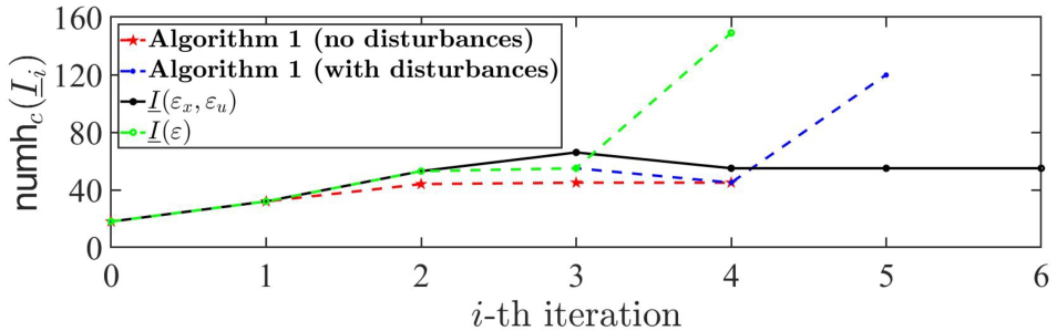
Finally, we also want to point out the difficulties in having a fair comparison between those discretization-based approaches and ours in terms of worst-case space complexity. It is well-known that the space complexities of discretization-based approaches grow exponentially with respect to the dimension of the state (and input) sets (see [27, Section 5-A] for detailed discussion) since they require the discretization of the original state and input sets in order to construct the finite state and input sets. On the one hand, the space complexity of our approaches does not have exponential growth regarding the dimensions since we do not require such discretization. On the other hand, the complexity of our approaches grows exponentially with respect to the number of iterations in the worst case. It is worth noting that, however, we do not observe such exponential growth in the case studies (see Figure 11). As a key insight, at each iteration step i∈ℕi\in\mathbb{N}, for all q,q′∈Qr​dq,q^{\prime}\in Q_{rd}, one can reduce 𝗇𝗎𝗆⁡(I¯i​(q,q′))\mathsf{num}(\underline{I}_{i}(q,q^{\prime})) and 𝗅𝖺𝗋𝗀⁡(I¯i​(q,q′))\mathsf{larg}(\underline{I}_{i}(q,q^{\prime})) in (5.4) and (5.5) by computing the minimal representations [53] and the union of (some of) the polytopes in I¯i​(q,q′)\underline{I}_{i}(q,q^{\prime}).

6. Case Study

To show the effectiveness of our results, we first simulate the running example with the HCI-based controllers, which have already been computed in Section 4. Then, we apply our results to a cruise control example. Finally, we compare our approaches with some currently existing tools in terms of computational time. The synthesis and simulation are performed on a computer equipped with Quad-Core Intel Core i7 (2.7 GHz) and 16 GB of RAM running macOS Big Sur (Version 11.5.2), using MATLAB2019b along with multi-parametric toolbox MPT [48] and optimization software MOSEK (version 9.3.6) [61]. It is also worth noting that controllers in both cases can be applied over an infinite time horizon. The numbers of time steps for the simulation are selected only for demonstration purposes.

6.1. Running Example

Here, we randomly select 10 different initial states from I¯∗​(q0,q0)\underline{I}^{*}(q_{0},q_{0}), I¯​(εx,εu)​(q0,q0)\underline{I}(\varepsilon_{x},\varepsilon_{u})(q_{0},q_{0}), and I¯​(ε)​(q0,q0)\underline{I}(\varepsilon)(q_{0},q_{0}) (cf. Figure 5 and Figure 6), respectively, and simulate the running example for 30 time steps. In the simulation, the disturbances affecting the system are randomly generated at each time instant following a uniform distribution within the disturbance set. The simulation results for the maximal HCI set, the (εx\varepsilon_{x},εu\varepsilon_{u})-contraction-based and ε\varepsilon-expansion-based approximation are shown in Figure 7. One can verify that the desired property is respected.

Refer to caption
Refer to caption
Figure 7. Simulation of the running example with the controllers associated with the maximal HCI set, the (εx\varepsilon_{x},εu\varepsilon_{u})-contraction-based approximation and the ε\varepsilon-expansion-based approximation.

6.2. Cruise Control

Here, we focus on a cruise control problem for a truck with a trailer as in Figure 8, with dynamics as in (2.2), where

A:=[0.8855−0.36280.36280.40810.46830.5317001.0000],B:=[0.10180.13720.5000],\displaystyle A:=\begin{bmatrix}\begin{smallmatrix}0.8855\,&-0.3628&0.3628\\ 0.4081\,&0.4683&0.5317\\ 0\,&0\,&1.0000\end{smallmatrix}\end{bmatrix}\!,\ B:=\begin{bmatrix}\begin{smallmatrix}0.1018\\ 0.1372\\ 0.5000\end{smallmatrix}\end{bmatrix}\!, (6.1)
Refer to caption
Figure 8. Cruise control problem for a truck with a trailer, with mt​r​a​i​l​e​r=4000m_{trailer}=4000kg the mass of the trailer, ks=4500k_{s}=4500N/kg and kd=4600k_{d}=4600Ns/m the constants for the spring-damper system, and dd the distance between the truck and the trailer, where d=0d=0m is the position at which there is no deformation on the spring.

x⁡(k)=[x1​(k);x2​(k);x3​(k)]x(k)=[x_{1}(k);x_{2}(k);x_{3}(k)] is the state of the system, in which x1​(k)x_{1}(k), x2​(k)x_{2}(k), and x3​(k)x_{3}(k) are the distance between the truck and the trailer, the velocity of the trailer, and the velocity of the truck, respectively. Moreover, u⁡(k)∈[−5,5]u(k)\in[-5,5]m/s2 denotes the acceleration of the truck that is used as the control input; and w⁡(k)∈[−0.04,0.04]×[−0.02,0.02]2w(k)\in[-0.04,0.04]\times[-0.02,0.02]^{2} denotes the exogenous disturbances encompassing the model uncertainty and unexpected interferences. The model as in (6.1) is adapted from [14] by discretizing it with a sampling time Δ​t=0.5​s\Delta t=0.5s and including exogenous disturbances.

Figure 9. DSA 𝒜q\mathcal{A}_{q} modeling ψq\psi_{q}, with alphabet Π={p1,p2,p3,\Pi=\{p_{1},p_{2},p_{3}, p4,p5}p_{4},p_{5}\}; labeling function L:X→ΠL:X\rightarrow\Pi with L⁡(x)=p1L(x)=p_{1} when x∈x\in [−1,1]×[5,35]×[15,25][-1,1]\times[5,35]\times[15,25], L⁡(x)=p2L(x)=p_{2} when x∈[−1,1]×x\in[-1,1]\times [5,35]×(25,35][5,35]\times(25,35], L⁡(x)=p3L(x)=p_{3} when x∈x\in [−1,1]×[5,35]×[5,35][-1,1]\times[5,35]\times[5,35], L⁡(x)=p4L(x)=p_{4} when x∈ℝ3\L−1​(p3)x\in\mathbb{R}^{3}\backslash L^{-1}(p_{3}), and L⁡(x)=p5L(x)=p_{5} when x∈ℝ3\(L−1​(p1)∪L−1​(p2))x\in\mathbb{R}^{3}\backslash(L^{-1}(p_{1})\cup L^{-1}(p_{2})); and accepting condition Acc={⟨E1,F1⟩}\text{Acc}=\{\langle E_{1},F_{1}\rangle\}, with E1={q3}E_{1}=\{q_{3}\}, F1=∅F_{1}=\emptyset. The temporal logics formula for ψq\psi_{q} is given by G⁡((p1​U​p2)∧(¬p​3))G((p_{1}Up_{2})\wedge(\neg p3)).

In this case study, the distance between the truck and the trailer should be within [−1,1][-1,1]m to protect the spring-damper system, and the velocity of the truck and the trailer should be within [5,35][5,35]m/s due to the traffic rules. Additionally, to increase the throughput of the road traffic, the truck is not allowed to move slower than 1515m/s unless it has moved faster than 2525m/s. Such a property, denoted by ψq\psi_{q}, can be modeled by a DSA 𝒜q\mathcal{A}_{q} as depicted in Figure 9. To synthesize controllers enforcing ψq\psi_{q}, we select E¯:=∪∀q′∈Q(q′,q2,X¯(q′,q2))\underline{E}:=\cup_{\forall q^{\prime}\in Q}\big(q^{\prime},q_{2},\underline{X}(q^{\prime},q_{2})\big). Additionally, to ensure the compactness of X¯\E¯\underline{X}\backslash\underline{E}, we slightly deflate X¯\E¯\underline{X}\backslash\underline{E} such that X¯\E¯​(q0,q1):=[−1,1]×[5,35]×[20+ϵ,35]\underline{X}\backslash\underline{E}(q_{0},q_{1}):=[-1,1]\times[5,35]\times[20+\epsilon,35], with ϵ=0.001\epsilon=0.001. The results of controller synthesis are summarized in Table 2. Then, we randomly select 10 initial states from I¯∗​(q0,q0)\underline{I}^{*}(q_{0},q_{0}), I¯​(εx,εu)​(q0,q0)\underline{I}(\varepsilon_{x},\varepsilon_{u})(q_{0},q_{0}), and I¯​(ε)​(q0,q0)\underline{I}(\varepsilon)(q_{0},q_{0}), respectively, and simulate the systems for 60 seconds (i.e. 120 time steps). Moreover, the disturbances are randomly generated at each time step following a uniform distribution within the disturbance set. The simulation results are shown in Figure 10, indicating that the desired property is enforced (note that trajectories of x3x_{3} become red after x3x_{3} has been larger than 2525m/s). Additionally, Figure 11 shows that there is no exponential growth as in (5.4) and (5.5) in this case study.

Table 2. Synthesizing controllers for the cruise control problem by computing: 1) maximal HCI set I¯∗\underline{I}^{*}; 2) contraction-based approximation I¯​(εx,εu)\underline{I}(\varepsilon_{x},\!\varepsilon_{u}) with n=3n\!=\!3 and εx=εu=0.036\varepsilon_{x}=\varepsilon_{u}\!=\!0.036; 3) expansion-based approximation I¯​(ε)\underline{I}(\varepsilon) with ε=0.002\varepsilon=0.002.
I¯∗\underline{I}^{*} I¯​(εx,εu)\underline{I}(\varepsilon_{x},\varepsilon_{u}) I¯​(ε)\underline{I}(\varepsilon)
Number of iterations 5 6 4
Computation time (s) 21.34 19.59 16.12
Number of hyperplanes 120 259 149
Refer to caption
Refer to caption
Refer to caption
Figure 10. Simulation of the cruise control problem
Refer to caption
Figure 11. Evolution of the number of hyperplanes required to characterize I¯i\underline{I}_{i}, denoted by 𝗇𝗎𝗆𝗁c​(I¯i)\mathsf{numh}_{c}(\underline{I}_{i}), as ii increases.

6.3. Comparison with Existing Results

Table 3. Comparison among the proposed HCI-based methods and existing results in terms of computation time for synthesizing controllers enforcing: 1) (Case 1) ψq\psi_{q} over system in (6.1) with disturbances; 2) (Case 2) ψq\psi_{q} over system in (6.1) without disturbances; 3) (Case 3) system in (6.1) with disturbances reaching a target set within 3 time steps.
Methods
Maximal
HCI-set
(εx\varepsilon_{x},εu\varepsilon_{u})-contraction ε\varepsilon-expansion ROCS TuLiP OmegaThreads CBF-based HJ-based
Case 1 21.34 s 19.59 s 16.12 s N/A >>6 h 2899.85 s N/A N/A
Case 2 2.92 s 7.44 s 7.04 s >>6 h >>6 h 1933.60 s N/A N/A
Case 3 51.02 s 86.27 s 44.30 s N/A >>6 h 7123.81 s N/A 415.15 s

In this subsection, we compare the proposed set-based approaches with existing results in terms of computation time for synthesizing controllers, including symbolic techniques (OmegaThreads [17] and TuLiP [62]), interval-analysis-based approaches (ROCS [63]), CBF-based approaches [34], and HJ-based approaches (helperOC [9] equipped with toolboxLS [64]). Moreover, since interval-based approaches do not handle systems with exogenous disturbances [27, Section 2.D], and HJ-based approaches do not handle ω\omega-regular properties, for a fair comparison among these approaches, we consider three different cases: 1) enforcing ψq\psi_{q} in Session 6.2 over the system in (6.1); 2) enforcing ψq\psi_{q} over the system in (6.1), but without exogenous disturbance; 3) ensuring the system in (6.1) reaches the region [−1,1]×[5,35]×[25,35][-1,1]\times[5,35]\times[25,35] from the region [−1,1]×[5,35]×[5,25][-1,1]\times[5,35]\times[5,25] within 3 time steps.

Following the same settings as in Table 2, we choose n=3n=3 and εx=εu=0.036\varepsilon_{x}\!=\!\varepsilon_{u}\!=\!0.036 to compute the (εx\varepsilon_{x},εu\varepsilon_{u})-contraction-based approximation of the maximal HCI-set, and select ε=0.002\varepsilon=0.002 to compute the ε\varepsilon-expansion-based approximation. For applying ROCS, we select ε=0.001\varepsilon=0.001 and μ=0.001\mu=0.001 as the lower bounds of discretization parameters for state and input sets, respectively, (see [27, Section 4-A] for their definitions) for a fair comparison with the setting of ε\varepsilon-expansion-based approach [27, Lemma 1 and Theorem 1]. Moreover, considering the limitation of our computer, 0.20.2 is used as the discritization parameter for discretizing the state and input sets when deploying OmegaThreads, TuLiP, and helperOC. The computation time for synthesizing controllers with different approaches is summarized in Table 3, which indicates that our approaches require less computation time than other ones. Concretely, >>6 h means that the corresponding synthesis procedures did not terminate within 6h, and that the actual computation time is undecided. Additionally, when applying OmegaThreads, no controller was found in all cases with the current discretization parameters. Therefore, smaller discretization parameters for the state and input sets are needed to potentially obtain controllers, which would, however, result in longer computation time. As for using CBF-based methods in [42], although we set the potential control barrier function, the multipliers, and the controller as polynomials of up to degree eight, no controller was found in any cases.

7. Conclusion

In this paper, we proposed for the first time a notion of so-called hybrid controlled invariant set (HCI set), based on which we synthesize controllers to enforce ω\omega-regular properties over linear control systems affected by bounded disturbances. Given a linear control system and a deterministic Streett automata (DSA) modeling the desired ω\omega-regular property, we first construct a product system between the linear control system and the DSA. Then, we compute the maximal HCI set by utilizing a set-based approach over the hybrid state set of the product system. Additionally, we provide two approaches to compute approximations of the maximal HCI sets within a finite number of iterations: one by deflating the original state and input sets, the other by expanding the disturbance set. The effectiveness of our methods is shown by two case studies, and by comparison with existing tools.

References

  • [1] P. Tabuada, Verification and control of hybrid systems: a symbolic approach, Springer Science & Business Media, 2009.
  • [2] A. Pnueli, The temporal logic of programs, in: Proceedings of the 18th Annual Symposium on Foundations of Computer Science, 1977, pp. 46–57.
  • [3] S. Maierhofer, P. Moosbrugger, M. Althoff, Formalization of intersection traffic rules in temporal logic, in: 2022 IEEE Intelligent Vehicles Symposium (IV), 2022, pp. 1135–1144.
  • [4] P. Yu, D. V. Dimarogonas, Distributed motion coordination for multirobot systems under LTL specifications, IEEE Transactions on Robotics 38 (2) (2022) 1047–1062.
  • [5] W. Thomas, Automata on infinite objects, in: Formal Models and Semantics, Elsevier, 1990, pp. 133–191.
  • [6] A. Pnueli, R. Rosner, On the synthesis of a reactive module, in: Proceedings of the 16th ACM SIGPLAN-SIGACT symposium on Principles of programming languages, 1989, pp. 179–190.
  • [7] P. J. Meyer, S. Sickert, M. Luttenberger, Strix: Explicit reactive synthesis strikes back!, in: Proceedings of the International Conference on Computer Aided Verification, 2018, pp. 578–586.
  • [8] J. Esparza, J. Křetínskỳ, J.-F. Raskin, S. Sickert, From LTL and limit-deterministic Büchi automata to deterministic parity automata, in: Proceedings of the International Conference on Tools and Algorithms for the Construction and Analysis of Systems, 2017, pp. 426–442.
  • [9] S. Bansal, M. Chen, S. Herbert, C. J. Tomlin, Hamilton-Jacobi reachability: A brief overview and recent advances, in: 2017 IEEE 56th Annual Conference on Decision and Control (CDC), IEEE, 2017, pp. 2242–2253.
  • [10] I. M. Mitchell, A. M. Bayen, C. J. Tomlin, A time-dependent Hamilton-Jacobi formulation of reachable sets for continuous dynamic games, IEEE Transactions on automatic control 50 (7) (2005) 947–957.
  • [11] M. Zamani, G. Pola, M. Mazo, P. Tabuada, Symbolic models for nonlinear control systems without stability assumptions, IEEE Transactions on Automatic Control 57 (7) (2011) 1804–1809.
  • [12] G. Pola, A. Girard, P. Tabuada, Approximately bisimilar symbolic models for nonlinear control systems, Automatica 44 (10) (2008) 2508–2516.
  • [13] G. Reissig, A. Weber, M. Rungger, Feedback refinement relations for the synthesis of symbolic controllers, IEEE Transactions on Automatic Control 62 (4) (2017) 1781–1796.
  • [14] M. Rungger, M. Mazo, P. Tabuada, Specification-guided controller synthesis for linear systems and safe linear-time temporal logic, in: Proceedings of the 16th international conference on Hybrid systems: computation and control, 2013, pp. 333–342.
  • [15] P. Tabuada, G. J. Pappas, Linear time logic control of discrete-time linear systems, IEEE Transactions on Automatic Control 51 (12) (2006) 1862–1877.
  • [16] M. Dutreix, J. Huh, S. Coogan, Abstraction-based synthesis for stochastic systems with omega-regular objectives, arXiv:2001.09236 (2020).
  • [17] M. Khaled, M. Zamani, Omegathreads: Symbolic controller design for ω\omega-regular objectives, in: Proceedings of the 24th ACM International Conference on Hybrid Systems: Computation and Control, 2021, pp. 1–7.
  • [18] A. Swikir, M. Zamani, Compositional synthesis of finite abstractions for networks of systems: A small-gain approach, Automatica 107 (2019) 551–561.
  • [19] M. Zamani, M. Arcak, Compositional abstraction for networks of control systems: A dissipativity approach, IEEE Transactions on Control of Network Systems 5 (3) (2018) 1003–1015.
  • [20] G. Pola, P. Pepe, M. D. Di Benedetto, Decentralized supervisory control of networks of nonlinear control systems, IEEE Transactions on Automatic Control 63 (9) (2017) 2803–2817.
  • [21] E. M. Wolff, U. Topcu, R. M. Murray, Automaton-guided controller synthesis for nonlinear systems with temporal logic, in: Proceedings of the IEEE/RSJ International Conference on Intelligent Robots and Systems, 2013, pp. 4332–4339.
  • [22] M. H. Zibaeenejad, J. Liu, Auditor product and controller synthesis for nondeterministic transition systems with practical LTL specifications, IEEE Transactions on Automatic Control 65 (10) (2019) 4281–4287.
  • [23] M. Dutreix, S. Coogan, Specification-guided verification and abstraction refinement of mixed monotone stochastic systems, IEEE Transactions on Automatic Control 66 (2020) 2975–2990.
  • [24] P.-J. Meyer, D. V. Dimarogonas, Compositional abstraction refinement for control synthesis, Nonlinear Analysis: Hybrid Systems 27 (2018) 437–451.
  • [25] Y. Li, J. Liu, Invariance control synthesis for switched nonlinear systems: An interval analysis approach, IEEE Transactions on Automatic Control 63 (7) (2017) 2206–2211.
  • [26] Y. Li, J. Liu, Robustly complete synthesis of memoryless controllers for nonlinear systems with reach-and-stay specifications, IEEE Transactions on Automatic Control 66 (2020) 1199–1206.
  • [27] Y. Li, Z. Sun, J. Liu, A specification-guided framework for temporal logic control of nonlinear systems, IEEE Transactions on Automatic Control (2022) 1–1.
  • [28] D. Bertsekas, Infinite time reachability of state-space regions by using feedback control, IEEE Transactions on Automatic Control 17 (5) (1972) 604–613.
  • [29] S. V. Rakovic, P. Grieder, M. Kvasnica, D. Q. Mayne, M. Morari, Computation of invariant sets for piecewise affine discrete time systems subject to bounded disturbances, in: Proceedings of the 43rd IEEE Conference on Decision and Control, Vol. 2, 2004, pp. 1418–1423.
  • [30] F. Blanchini, S. Miani, Set-Theoretic Methods in Control, Birkhäuser, 2015.
  • [31] M. Rungger, P. Tabuada, Computing robust controlled invariant sets of linear systems, IEEE Transactions on Automatic Control 62 (7) (2017) 3665–3670.
  • [32] S. Liu, M. Zamani, Compositional synthesis of almost maximally permissible safety controllers, in: Proceedings of the American Control Conference, 2019, pp. 1678–1683.
  • [33] P. Wieland, F. Allgöwer, Constructive safety using control barrier functions, IFAC Proceedings Volumes 40 (12) (2007) 462–467.
  • [34] N. Jahanshahi, A. Lavaei, M. Zamani, Compositional construction of safety controllers for networks of continuous-space POMDPs, arXiv:2103.05906 (2021).
  • [35] A. Nejati, S. Soudjani, M. Zamani, Compositional construction of control barrier certificates for large-scale stochastic switched systems, IEEE Control Systems Letters 4 (4) (2020) 845–850.
  • [36] M. Jankovic, Control barrier functions for constrained control of linear systems with input delay, in: Proceedings of the Annual American Control Conference, 2018, pp. 3316–3321.
  • [37] A. D. Ames, X. Xu, J. W. Grizzle, P. Tabuada, Control barrier function based quadratic programs for safety critical systems, IEEE Transactions on Automatic Control 62 (8) (2016) 3861–3876.
  • [38] P. Jagtap, S. Soudjani, M. Zamani, Formal synthesis of stochastic systems via control barrier certificates, IEEE Transactions on Automatic Control 66 (2020) 3097–3110. arXiv:1905.04585v1.
  • [39] M. Anand, A. Lavaei, M. Zamani, From small-gain theory to compositional construction of barrier certificates for large-scale stochastic systems, arXiv:2101.06916 (2021).
  • [40] P. Jagtap, A. Swikir, M. Zamani, Compositional construction of control barrier functions for interconnected control systems, in: Proceedings of the 23rd International Conference on Hybrid Systems: Computation and Control, 2020.
  • [41] M. Srinivasan, S. Coogan, M. Egerstedt, Control of multi-agent systems with finite time control barrier certificates and temporal logic, in: Proceedings of the IEEE Conference on Decision and Control, 2018, pp. 1991–1996.
  • [42] M. Anand, A. Lavaei, M. Zamani, Compositional synthesis of control barrier certificates for networks of stochastic systems against ω\omega-regular specifications, arXiv:2103.02226 (2021).
  • [43] J. J. Choi, D. Lee, K. Sreenath, C. J. Tomlin, S. L. Herbert, Robust control barrier-value functions for safety-critical control, arXiv:2104.02808 (2021).
  • [44] B. Zhong, M. Zamani, M. Caccamo, A set-based approach for synthesizing controllers enforcing ω\omega-regular properties over uncertain linear control systems, in: Proceedings of the American Control Conference, 2022, to appear.
  • [45] R. S. Streett, Propositional dynamic logic of looping and converse is elementarily decidable, Information and control 54 (1-2) (1982) 121–141.
  • [46] C. Baier, J.-P. Katoen, Principles of model checking, MIT press, 2008.
  • [47] B. Grünbaum, Convex Polytopes, Vol. 221, Springer Science & Business Media, 2003.
  • [48] M. Herceg, M. Kvasnica, C. N. Jones, M. Morari, Multi-parametric toolbox 3.0, in: Proceedings of the European Control Conference, Zürich, Switzerland, 2013, pp. 502–510, http://control.ee.ethz.ch/~mpt.
  • [49] A. Löhne, B. Weißing, Equivalence between polyhedral projection, multiple objective linear programming and vector linear programming, Mathematical Methods of Operations Research 84 (2) (2016) 411–426.
  • [50] R. Vidal, S. Schaffert, J. Lygeros, S. Sastry, Controlled invariance of discrete time systems, in: Proceedings of the International Workshop on Hybrid Systems: Computation and Control, 2000, pp. 437–451.
  • [51] P. O. Gutman, M. Cwikel, Admissible sets and feedback control for discrete-time linear dynamical systems with bounded controls and states, IEEE transactions on Automatic Control 31 (4) (1986) 373–376.
  • [52] E. C. Kerrigan, Robust constraint satisfaction: Invariant sets and predictive control, Ph.D. thesis, University of Cambridge (2001).
  • [53] M. Baotic, Polytopic computations in constrained optimal control, Automatika, Journal for Control, Measurement, Electronics, Computing and Communications 50 (2009) 119–134.
  • [54] S. V. Rakovic, E. C. Kerrigan, D. Q. Mayne, J. Lygeros, Reachability analysis of discrete-time systems with disturbances, IEEE Transactions on Automatic Control 51 (4) (2006) 546–561.
  • [55] C. Jones, E. C. Kerrigan, J. Maciejowski, Equality set projection: A new algorithm for the projection of polytopes in halfspace representation, Tech. rep. (2004).
  • [56] M. I. Karavelas, E. Tzanaki, The maximum number of faces of the Minkowski sum of two convex polytopes, Discrete and Computational Geometry 55 (4) (2016) 748–785.
  • [57] H. Yu, D. Monniaux, An efficient parametric linear programming solver and application to polyhedral projection, in: International Static Analysis Symposium, Springer, 2019, pp. 203–224.
  • [58] A. Bemporad, K. Fukuda, F. D. Torrisi, Convexity recognition of the union of polyhedra, Computational Geometry 18 (3) (2001) 141–154.
  • [59] M. Van Kreveld, O. Schwarzkopf, M. de Berg, M. Overmars, Computational geometry algorithms and applications, 3rd Edition, Springer, 2008.
  • [60] C. Weibel, Minkowski sums of polytopes: combinatorics and computation, Ph.D. thesis, EPFL (2007).
  • [61] MOSEK ApS, The MOSEK optimization toolbox for MATLAB manual. Version 9.3.6 (2019).
    URL http://docs.mosek.com/9.0/toolbox/index.html
  • [62] I. Filippidis, S. Dathathri, S. C. Livingston, N. Ozay, R. M. Murray, Control design for hybrid systems with tulip: The temporal logic planning toolbox, in: 2016 IEEE Conference on Control Applications (CCA), IEEE, 2016, pp. 1030–1041.
  • [63] Y. Li, J. Liu, ROCS: A robustly complete control synthesis tool for nonlinear dynamical systems, in: Proceedings of the 21st International Conference on Hybrid Systems: Computation and Control, 2018, pp. 130–135.
  • [64] I. M. Mitchell, J. A. Templeton, A toolbox of Hamilton-Jacobi solvers for analysis of nondeterministic continuous and hybrid systems, in: International workshop on Hybrid Systems: Computation and Control, Springer, 2005, pp. 480–494.

Appendix A Proof of Statements

A.1. Proof of Proposition 3.7 and Theorem 3.11

We first show the results for Proposition 3.7.

Proof of Proposition 3.7 Consider any controller sequence μ′={μ0′,μ1′,…,μi′,…}\mu^{\prime}=\{\mu^{\prime}_{0},\mu^{\prime}_{1},\ldots,\mu^{\prime}_{i},\ldots\}, with i∈ℕi\in\mathbb{N}, associated with I¯\underline{I} such that for any initial state x¯​(0)∈I¯\underline{x}(0)\in\underline{I}, and infinite state sequence ξ¯={x¯​(0),x¯​(1),…,x¯​(i),…}\underline{\xi}=\{\underline{x}(0),\underline{x}(1),\ldots,\underline{x}(i),\ldots\}, one has x¯​(i)∈I¯,∀i∈ℕ\underline{x}(i)\!\in\!\underline{I},\forall i\!\in\!\mathbb{N}, when μ′\mu^{\prime} is applied. Note that such controller sequence exists according to the definition of the HCI set as in Definition 3.5. Hence, at time instant i=0i=0, ∀x¯∈I¯\forall\underline{x}\in\underline{I}, ∀w∈W¯\forall w\in\underline{W}, one gets x¯′:=f¯​(x¯,u,w)∈I¯\underline{x}^{\prime}:=\underline{f}(\underline{x},u,w)\in\underline{I} with u=μ0′​(x¯)u=\mu^{\prime}_{0}(\underline{x}). Since one has x¯′∈I¯\underline{x}^{\prime}\in\underline{I}, then ∀w′∈W¯\forall w^{\prime}\in\underline{W}, we again have x¯′′:=f¯​(x¯′,u,w′)∈I¯\underline{x}^{\prime\prime}:=\underline{f}(\underline{x}^{\prime},u,w^{\prime})\in\underline{I} with u=μ0′​(x¯)u=\mu^{\prime}_{0}(\underline{x}) at time instant i=1i=1. Therefore, one can verify that with the sequence of controller μ′′:={μ0′′,\mu^{\prime\prime}:=\{\mu^{\prime\prime}_{0}, μ1′′,…,μi′′,…}\mu^{\prime\prime}_{1},\ldots,\mu^{\prime\prime}_{i},\ldots\} with μi′′=μ0′\mu^{\prime\prime}_{i}=\mu^{\prime}_{0}, ∀i∈ℕ\forall i\in\mathbb{N}, one also has x¯​(i)∈I¯,∀i∈ℕ\underline{x}(i)\!\in\!\underline{I},\forall i\!\in\!\mathbb{N}, when μ′′\mu^{\prime\prime} is utilized. Note that μ′′\mu^{\prime\prime} is a stationary controller as in Definition 3.6, which completes the proof.■\hfill\blacksquare

Next, we proceed with showing Theorem 3.11, for which some additional definitions and lemmas are required. First, we define a set

G(X¯′):={(x¯,u)∈X¯×U¯|∀w∈W¯,f¯(x¯,u,w)∈X¯′},\displaystyle G(\underline{X}^{\prime})\!:=\!\{(\underline{x},u)\!\in\!\underline{X}\times\underline{U}~|~\forall w\in\underline{W},\underline{f}(\underline{x},u,w)\!\in\!\underline{X}^{\prime}\}, (A.1)

where X¯′⊆X¯\underline{X}^{\prime}\subseteq\underline{X}. Accordingly, consider I¯0\underline{I}_{0} along with the iteration of I¯i\underline{I}_{i} as in (3.11), we define GiG_{i} with i∈ℕ>0i\in\mathbb{N}_{>0} as:

G1​(I¯0)\displaystyle G_{1}(\underline{I}_{0}) :=G⁡(I¯0);\displaystyle:=G(\underline{I}_{0}); (A.2)
Gi​(I¯0)\displaystyle G_{i}(\underline{I}_{0}) :=G⁡(I¯i−1),i≥2.\displaystyle:=G(\underline{I}_{i-1}),\,i\geq 2. (A.3)

Now, based on theses definitions, we propose Lemma A.1 and Lemma A.2, which are also necessary for showing the proof of Theorem 3.11.

Lemma A.1.

Consider a dtLCS SS as in (2.2), a DSA 𝒜\mathcal{A} modeling the desired ω\omega-regular property, and the product dtLCS S⊗𝒜=(X¯,X¯0,U¯,W¯,f¯)S\otimes\mathcal{A}=(\underline{X},\underline{X}_{0},\underline{U},\underline{W},\underline{f}) such that Assumption 3.10 holds. Then, Gi​(I¯0)G_{i}(\underline{I}_{0}) are compact for all i∈ℕ>0i\in\mathbb{N}_{>0}, with GiG_{i} as defined in (A.2) and (A.3), and I¯0\underline{I}_{0} as in (3.11).

Proof of Lemma A.1 In case that Gi​(I¯0)=∅G_{i}(\underline{I}_{0})=\emptyset, the assertion of Lemma A.1 holds trivially. Therefore, we assume that Gi​(I¯0)≠∅G_{i}(\underline{I}_{0})\neq\emptyset, for all i∈ℕ>0i\in\mathbb{N}_{>0}. To this end, we first show that I¯i\underline{I}_{i} are compact for all i∈ℕi\in\mathbb{N}. Then, we show that Gi​(I¯)G_{i}(\underline{I}) is compact when I¯\underline{I} is compact, and the compactness of (Gi​(I¯0))i∈ℕ>0(G_{i}(\underline{I}_{0}))_{i\in\mathbb{N}_{>0}} follows by the compactness of (I¯i)i∈ℕ(\underline{I}_{i})_{i\in\mathbb{N}}. Firstly, I¯0\underline{I}_{0} as in (3.11) is compact according to Assumption 3.10. Since intersection of two compact sets are still compact, we show the compactness of (I¯i)i∈ℕ(\underline{I}_{i})_{i\in\mathbb{N}} by showing P​(I¯)\textbf{P}(\underline{I}) as in (3.13) is compact if I¯\underline{I} is compact. For this purpose, we rewrite P​(I¯)\textbf{P}(\underline{I}) as P(I¯)={x¯∈X¯|∃u∈U¯, s.t. f¯(x¯,u,𝟎n)∈I¯′}\textbf{P}(\underline{I})=\{\underline{x}\in\underline{X}~|~\exists u\in\underline{U},\text{ s.t. }\underline{f}(\underline{x},u,\mathbf{0}_{n})\in\underline{I}^{\prime}\}, with I¯′\underline{I}^{\prime} a bounded set being defined as I¯′={x¯′|{x¯′}⊕W¯⊆I¯}\underline{I}^{\prime}=\{\underline{x}^{\prime}~|~\{\underline{x}^{\prime}\}\oplus\underline{W}\subseteq\underline{I}\}. Consider any x¯′′:=(q,q′,x′)∉I¯′\underline{x}^{\prime\prime}:=(q,q^{\prime},x^{\prime})\notin\underline{I}^{\prime}. By definition of I¯′\underline{I}^{\prime}, there exists at least one w∈W¯w\in\underline{W} such that one gets z¯:=(q,q′,x′+w)∉I¯\underline{z}:=(q,q^{\prime},x^{\prime}+w)\notin\underline{I}. Since I¯\underline{I} is compact (and therefore closed), then there exists an open ball 𝖡\mathsf{B} in the sense of the distance as defined in (3.7) centered at (q,q′,0)(q,q^{\prime},0) such that (z¯+𝖡)∩I¯=∅(\underline{z}+\mathsf{B})\cap\underline{I}=\emptyset, with z¯+𝖡\underline{z}+\mathsf{B} denotes the Minkowski sum between z¯\underline{z} and 𝖡\mathsf{B}. Accordingly, for any x¯′′:=(q,q′,x′)∉I¯′\underline{x}^{\prime\prime}:=(q,q^{\prime},x^{\prime})\notin\underline{I}^{\prime}, one gets (x¯′′+𝖡)∩I¯′=∅(\underline{x}^{\prime\prime}+\mathsf{B})\cap\underline{I}^{\prime}=\emptyset, which implies that I¯′\underline{I}^{\prime} is closed. Therefore, ∀q,q′∈Q\forall q,q^{\prime}\in Q such that I¯′​(q,q′)≠∅\underline{I}^{\prime}(q,q^{\prime})\neq\emptyset, I¯′​(q,q′)\underline{I}^{\prime}(q,q^{\prime}) is closed and bounded (and therefore compact). Note that QQ is a finite set, and finite union of compact sets is still compact. Hence, it is straightforward that I¯′=∪q,q′∈QI¯′(q,q′)\underline{I}^{\prime}=\cup_{q,q^{\prime}\in Q}\underline{I}^{\prime}(q,q^{\prime}) is also compact. Since the dynamics of dtLCS SS as in (2.2) is continuous, mapping f¯\underline{f} is also continuous. Then, the compactness of P​(I¯)\textbf{P}(\underline{I}) follows by the compactness of U¯\underline{U}, I¯\underline{I}, and I¯′\underline{I}^{\prime}.

As for the compactness of Gi​(I¯)G_{i}(\underline{I}) given I¯\underline{I} is compact, we rewrite Gi​(I¯)G_{i}(\underline{I}) as in (A.1) as G⁡(I¯)={(x¯,u)∈X¯×U¯|f¯​(x¯,u,𝟎n)∈I¯′}G(\underline{I})\!=\!\{(\underline{x},u)\!\in\!\underline{X}\times\underline{U}~|~\underline{f}(\underline{x},u,\mathbf{0}_{n})\in\underline{I}^{\prime}\}. Then, the compactness of G⁡(I¯)G(\underline{I}) can be proved similarly to that of the compactness of P​(I¯)\textbf{P}(\underline{I}), which completes the proof. ■\hfill\blacksquare

Lemma A.2.

Consider GiG_{i} as defined in (A.2) and (A.3), and I¯0\underline{I}_{0} as in (3.11). We have

πX¯​(⋂i=1∞Gi​(I¯0))=limi→∞I¯i,\displaystyle\pi_{\underline{X}}\Big(\bigcap_{i=1}^{\infty}G_{i}(\underline{I}_{0})\Big)=\lim\limits_{i\rightarrow\infty}\underline{I}_{i}, (A.4)

with πX¯​(Gi​(I¯0))\pi_{\underline{X}}(G_{i}(\underline{I}_{0})) the projection of Gi​(I¯0)G_{i}(\underline{I}_{0}) on to X¯\underline{X}.

Proof of Lemma A.2 To show Lemma A.2, we show that 1) πX¯​(⋂i=1∞Gi​(I¯0))⊆limi→∞I¯i\pi_{\underline{X}}\Big(\bigcap_{i=1}^{\infty}G_{i}(\underline{I}_{0})\Big)\subseteq\lim\limits_{i\rightarrow\infty}\underline{I}_{i}; 2) limi→∞I¯i⊆πX¯​(⋂i=1∞Gi​(I¯0))\lim\limits_{i\rightarrow\infty}\underline{I}_{i}\subseteq\pi_{\underline{X}}\Big(\bigcap_{i=1}^{\infty}G_{i}(\underline{I}_{0})\Big).

First, we show that

πX¯​(⋂i=1∞Gi​(I¯0))⊆limi→∞I¯i,\pi_{\underline{X}}\Big(\bigcap_{i=1}^{\infty}G_{i}(\underline{I}_{0})\Big)\subseteq\lim\limits_{i\rightarrow\infty}\underline{I}_{i}, (A.5)

holds. Let’s denote by ξ¯={x¯​(0),x¯​(1),…,x¯​(i),…}\underline{\xi}=\{\underline{x}(0),\underline{x}(1),\ldots,\underline{x}(i),\ldots\} an infinite state sequence of S⊗𝒜S\otimes\mathcal{A}. On one hand, according to the definition of Gi​(I¯0)G_{i}(\underline{I}_{0}), πX¯​(⋂i=1∞Gi​(I¯0))\pi_{\underline{X}}\Big(\bigcap_{i=1}^{\infty}G_{i}(\underline{I}_{0})\Big) denotes the set of x¯∈I¯0\underline{x}\in\underline{I}_{0}, from which there exists a stationary controller μ¯={μ,μ,…}\bar{\mu}=\{\mu,\mu,\ldots\} such that x¯​(i)∈I¯0\underline{x}(i)\in\underline{I}_{0}, for all i∈ℕi\in\mathbb{N}. On the other hand, according to the iteration in (3.11), limi→∞I¯i\lim\limits_{i\rightarrow\infty}\underline{I}_{i} denotes the set of all x¯∈I¯0\underline{x}\in\underline{I}_{0}, from which there exists a controller (either stationary or non-stationary) μ¯′={μ1′,μ2′,…}\bar{\mu}^{\prime}=\{\mu^{\prime}_{1},\mu^{\prime}_{2},\ldots\} such that x¯​(i)∈I¯0\underline{x}(i)\in\underline{I}_{0} for all i∈ℕi\in\mathbb{N}. Therefore, (A.5) holds.

Next, we show that

limi→∞I¯i⊆πX¯​(⋂i=1∞Gi​(I¯0)),\lim\limits_{i\rightarrow\infty}\underline{I}_{i}\subseteq\pi_{\underline{X}}\Big(\bigcap_{i=1}^{\infty}G_{i}(\underline{I}_{0})\Big), (A.6)

holds. According to the definition of Gi​(I¯0)G_{i}(\underline{I}_{0}) and I¯i\underline{I}_{i}, one gets

limi→∞I¯i=⋂i=1∞πX¯​(Gi​(I¯0)).\displaystyle\lim\limits_{i\rightarrow\infty}\underline{I}_{i}=\bigcap_{i=1}^{\infty}\pi_{\underline{X}}(G_{i}(\underline{I}_{0})). (A.7)

Therefore, we proceed with proving

⋂i=1∞πX¯​(Gi​(I¯0))⊆πX¯​(⋂i=1∞Gi​(I¯0)).\bigcap_{i=1}^{\infty}\pi_{\underline{X}}(G_{i}(\underline{I}_{0}))\subseteq\pi_{\underline{X}}\Big(\bigcap_{i=1}^{\infty}G_{i}(\underline{I}_{0})\Big). (A.8)

Consider an x¯∈⋂i=1∞πX¯​(Gi​(I¯0))\underline{x}\in\bigcap_{i=1}^{\infty}\pi_{\underline{X}}(G_{i}(\underline{I}_{0})). Then, there exists a sequence {ui}i∈ℕ\{u_{i}\}_{i\in\mathbb{N}}, such that (x¯,ui)∈Gi​(I¯0)(\underline{x},u_{i})\in G_{i}(\underline{I}_{0}), ∀i∈ℕ\forall i\in\mathbb{N}. On one hand, according to the computation of I¯i\underline{I}_{i}, i∈ℕi\in\mathbb{N} as in (3.11), it is straightforward that I¯0⊇I¯1⊇…⊇I¯i⊇…\underline{I}_{0}\supseteq\underline{I}_{1}\supseteq\ldots\supseteq\underline{I}_{i}\supseteq\ldots. Then, considering the definition of Gi​((I¯0))G_{i}((\underline{I}_{0})) as in (A.2) and (A.3), for all i∈ℕ>0i\in\mathbb{N}_{>0}, one has G1​(I¯0)⊇G2​(I¯0)⊇…⊇Gi​(I¯0)⊇…G_{1}(\underline{I}_{0})\supseteq G_{2}(\underline{I}_{0})\supseteq\ldots\supseteq G_{i}(\underline{I}_{0})\supseteq\ldots. Hence, ∀i′≥i>0\forall i^{\prime}\geq i>0, if one has (x¯,ui′)∈Gi′​(I¯0)(\underline{x},u_{i^{\prime}})\in G_{i^{\prime}}(\underline{I}_{0}), then one gets (x¯,ui′)∈Gi​(I¯0)(\underline{x},u_{i^{\prime}})\in G_{i}(\underline{I}_{0}). On the other hand, since Gi​(I¯0)G_{i}(\underline{I}_{0}) are compact according to Lemma A.1, any sequences of elements within Gi​(I¯)G_{i}(\underline{I}) has at least one limit point (x¯,u)∈Gi​(I¯)(\underline{x},u)\in G_{i}(\underline{I}). This indicate that ∃(x¯,u)∈Gi​(I¯0)\exists(\underline{x},u)\in G_{i}(\underline{I}_{0}), ∀i∈ℕ>0\forall i\in\mathbb{N}_{>0}, i.e., one has (x¯,u)∈⋂i=1∞Gi​(I¯0)(\underline{x},u)\in\bigcap_{i=1}^{\infty}G_{i}(\underline{I}_{0}). This indicates that x¯∈πX¯​(⋂i=1∞Gi​(I¯0))\underline{x}\in\pi_{\underline{X}}\Big(\bigcap_{i=1}^{\infty}G_{i}(\underline{I}_{0})\Big), which implies that (A.8) holds, and as a result (A.6) holds. Then, we complete the proof by combining (A.5) and (A.6). ■\hfill\blacksquare

With Lemma A.1, Lemma A.2, and Proposition 3.7, we are ready to prove Theorem 3.11.

Proof of Theorem 3.11 In case that I¯∗=∅\underline{I}^{*}=\emptyset, then there exists i∈ℕi\in\mathbb{N} such that for all i′≥ii^{\prime}\geq i, I¯i′=∅\underline{I}_{i^{\prime}}=\emptyset according the iteration as in (3.11). Therefore, I¯∗=limi→∞I¯i\underline{I}^{*}=\lim\limits_{i\rightarrow\infty}\underline{I}_{i} holds trivially. This assertion can be proved by contradiction. Suppose I¯′:=limi→∞I¯i≠∅\underline{I}^{\prime}:=\lim\limits_{i\rightarrow\infty}\underline{I}_{i}\neq\emptyset. Then, ∀x¯∈I¯′\forall\underline{x}\in\underline{I}^{\prime}, there exists an infinite sequence of inputs ξu​(u⁡(0),u⁡(1),…)\xi_{u}(u(0),u(1),\ldots) such that the corresponding infinite state sequence ξx​(x⁡(0),x⁡(1),…)\xi_{x}(x(0),x(1),\ldots) can be enforced within I¯0\underline{I}_{0}, i.e., I¯′\underline{I}^{\prime} is an HCI set for S⊗𝒜S\otimes\mathcal{A}. However, this is contradictory to the fact that the maximal HCI set I¯∗\underline{I}^{*} is empty.

Next, we consider the case in which I¯∗≠∅\underline{I}^{*}\neq\emptyset. Considering (A.7), we first show that ⋂i=1∞πX¯​(Gi​(I¯0))\bigcap_{i=1}^{\infty}\pi_{\underline{X}}(G_{i}(\underline{I}_{0})) is an HCI set for S⊗𝒜S\otimes\mathcal{A}, which implies that

⋂i=1∞πX¯​(Gi​(I¯0))⊆I¯∗,\bigcap_{i=1}^{\infty}\pi_{\underline{X}}(G_{i}(\underline{I}_{0}))\subseteq\underline{I}^{*}, (A.9)

holds. Consider a controller μ:X¯→U¯\mu:\underline{X}\rightarrow\underline{U} such that for all x¯∈⋂i=1∞πX¯​(Gi​(I¯0))\underline{x}\in\bigcap_{i=1}^{\infty}\pi_{\underline{X}}(G_{i}(\underline{I}_{0})), (x¯,μ⁡(x¯))∈⋂i=1∞Gi​(I¯0)(\underline{x},\mu(\underline{x}))\in\bigcap_{i=1}^{\infty}G_{i}(\underline{I}_{0}) (such controller exists according to Lemma A.2 by considering (A.4) and (A.7)). Then, by definition of Gi​(I¯0)G_{i}(\underline{I}_{0}), ∀x¯∈⋂i=1∞πX¯​(Gi​(I¯0))\forall\underline{x}\in\bigcap_{i=1}^{\infty}\pi_{\underline{X}}(G_{i}(\underline{I}_{0})), and ∀w∈W¯\forall w\in\underline{W}, one gets f¯​(x¯,μ⁡(x¯),w)∈⋂i=1∞πX¯​(Gi​(I¯0))\underline{f}(\underline{x},\mu(\underline{x}),w)\in\bigcap_{i=1}^{\infty}\pi_{\underline{X}}(G_{i}(\underline{I}_{0})). Therefore, ⋂i=1∞πX¯​(Gi​(I¯0))\bigcap_{i=1}^{\infty}\pi_{\underline{X}}(G_{i}(\underline{I}_{0})) is an HCI set for S⊗𝒜S\otimes\mathcal{A} so that (A.9) holds according to Definition 3.5.

Next, we proceed with showing that

I¯∗⊆⋂i=1∞πX¯​(Gi​(I¯0)),\underline{I}^{*}\subseteq\bigcap_{i=1}^{\infty}\pi_{\underline{X}}(G_{i}(\underline{I}_{0})), (A.10)

also holds. On one hand, according to Proposition 3.7, there exists a HCI-based controller μ\mu, such that for all x¯∈I¯∗\underline{x}\in\underline{I}^{*}, and for all w∈W¯w\in\underline{W}, one gets f¯​(x¯,μ⁡(x¯),w)∈I¯∗\underline{f}(\underline{x},\mu(\underline{x}),w)\in\underline{I}^{*}. On the other hand, by definition of Gi​(I¯0)G_{i}(\underline{I}_{0}) and the HCI-based controller, one has (x¯,μ⁡(x¯))∈⋂i=1∞Gi​(I¯0)(\underline{x},\mu(\underline{x}))\in\bigcap_{i=1}^{\infty}G_{i}(\underline{I}_{0}), indicating that x¯∈πX¯​(⋂i=1∞Gi​(I¯0))\underline{x}\in\pi_{\underline{X}}\Big(\bigcap_{i=1}^{\infty}G_{i}(\underline{I}_{0})\Big). Meanwhile, by (A.4) and (A.7), one has x¯∈⋂i=1∞πX¯​(Gi​(I¯0))\underline{x}\in\bigcap_{i=1}^{\infty}\pi_{\underline{X}}(G_{i}(\underline{I}_{0})), and therefore (A.10) also holds. Then, we are able to complete the proof by combining (A.7), (A.9), and (A.10). ■\hfill\blacksquare

A.2. Proof of Lemma 4.3 and Corollary 4.4

First, we propose Proposition A.3 that facilitates the proof of Lemma 4.3 and Corollary 4.4.

Proposition A.3.

If ∃cx,cu∈ℝ>0\exists c_{x},c_{u}\in\mathbb{R}_{>0} and n′∈ℕn^{\prime}\in\mathbb{N} such that for all x∈ℝnx\in\mathbb{R}^{n}, there exists ν:[0,n′]→ℝm\nu:[0,n^{\prime}]\rightarrow\mathbb{R}^{m} with which the following conditions hold:

  • •

    (Cd.1) ξx​(0)=x\xi_{x}(0)=x and ξx​(n′)=𝟎n\xi_{x}(n^{\prime})=\mathbf{0}_{n} with ξx​(k+1)=A​ξx​(k)+B​ν​(k)\xi_{x}(k+1)=A\xi_{x}(k)+B\nu(k) for all k∈[0,n′]k\in[0,n^{\prime}];

  • •

    (Cd.2) ν⁡(k)≤cu​|x|\nu(k)\leq c_{u}|x| holds for all k∈[0,n′]k\in[0,n^{\prime}];

  • •

    (Cd.3) ξx​(k)≤cx​|x|\xi_{x}(k)\leq c_{x}|x| holds for all k∈[0,n′]k\in[0,n^{\prime}];

then, for all γ∈ℝ>0\gamma\in\mathbb{R}_{>0}, one has γ​𝔹n⊆𝒩n′​(εx,εu)\gamma\mathbb{B}^{n}\subseteq\mathcal{N}_{n^{\prime}}(\varepsilon_{x},\varepsilon_{u}), with εx=cx​γ\varepsilon_{x}=c_{x}\gamma and εu=cu​γ\varepsilon_{u}=c_{u}\gamma.

Proof of Proposition A.3 According to Definition 4.2, (Cd.1) in Proposition A.3 indicates that there exists some εx′,εu′∈ℝ>0\varepsilon^{\prime}_{x},\varepsilon^{\prime}_{u}\in\mathbb{R}_{>0} such that ξx​(t)∈𝒩n′−t​(εx′,εu′)\xi_{x}(t)\in\mathcal{N}_{n^{\prime}-t}(\varepsilon^{\prime}_{x},\varepsilon^{\prime}_{u}), and then (Cd.2) as well as (Cd.3) guarantee that ξx​(t)∈𝒩n′−t​(εx,εu)\xi_{x}(t)\in\mathcal{N}_{n^{\prime}-t}(\varepsilon_{x},\varepsilon_{u}) with εx=cx​|x|\varepsilon_{x}=c_{x}|x| and εu=cu​|u|\varepsilon_{u}=c_{u}|u|. Therefore, one has x∈|x|​𝔹n⊆𝒩n′​(εx,εu)x\in|x|\mathbb{B}^{n}\subseteq\mathcal{N}_{n^{\prime}}(\varepsilon_{x},\varepsilon_{u}), which completes the proof.■\hfill\blacksquare

Now, we are ready to show the proof of Lemma 4.3.

Proof of Lemma 4.3 The proof of Lemma 4.3 is given by leveraging Proposition A.3. Concretely, we show the existence of cxc_{x} and cuc_{u} when n′=nn^{\prime}=n such that (Cd.1), (Cd.2) and (Cd.3) are fulfilled. Considering any x∈ℝnx\in\mathbb{R}^{n}, (Cd.1) requires that there exists a control sequence

ν=[ν​(n−1)T;ν​(n−2)T;…;ν​(0)T],\nu=[\nu(n-1)^{T};\nu(n-2)^{T};\ldots;\nu(0)^{T}], (A.11)

with ν⁡(k)∈ℝm\nu(k)\in\mathbb{R}^{m} for all k∈[0,n−1]k\in[0,n-1], such that ξx​(n)=An​x+𝒞​ν=𝟎n\xi_{x}(n)=A^{n}x+\mathcal{C}\nu=\mathbf{0}_{n}, with 𝒞=[B;A​B;…;An−1​B]T\mathcal{C}=[B;AB;\ldots;A^{n-1}B]^{T} the controllability matrix. Since (A,B)(A,B) is controllable, one has r​a​n​k​(𝒞)=nrank(\mathcal{C})=n, indicating the existence of such control sequence. Therefore, (Cd.1) holds. Let 𝒞′∈ℝn×n\mathcal{C}^{\prime}\in\mathbb{R}^{n\times n} be a matrix that contains nn linearly independent columns of 𝒞\mathcal{C}. Here, we select ν\nu as in (A.11) by setting the entries ν¯\underline{\nu} of ν\nu associated with 𝒞′\mathcal{C}^{\prime} of 𝒞\mathcal{C} as ν¯=−(𝒞′)−1​An​x\underline{\nu}=-(\mathcal{C}^{\prime})^{-1}A^{n}x, and the remaining entries of ν\nu as zero. Accordingly, one can verify that ξx​(n)=An​x+𝒞​ν=𝟎n\xi_{x}(n)=A^{n}x+\mathcal{C}\nu=\mathbf{0}_{n} holds with such ν\nu. In this case, since |ν¯|≤|(𝒞′)−1​An|​|x||\underline{\nu}|\leq|(\mathcal{C}^{\prime})^{-1}A^{n}||x| holds, (Cd.2) also holds with

cu=|(𝒞′)−1​An|.c_{u}=|(\mathcal{C}^{\prime})^{-1}A^{n}|. (A.12)

Meanwhile, by applying the same ν\nu, one obtains ξx​(k)=Ak​x+∑t′=0k−1Ak−t′−1​B​ν​(t′)\xi_{x}(k)=A^{k}x+\sum_{t^{\prime}=0}^{k-1}A^{k-t^{\prime}-1}B\nu(t^{\prime}). Accordingly, one has

|ξx​(k)|\displaystyle|\xi_{x}(k)| =|Ak​x+∑t′=0k−1Ak−t′−1​B​ν​(t′)|\displaystyle=|A^{k}x+\sum_{t^{\prime}=0}^{k-1}A^{k-t^{\prime}-1}B\nu(t^{\prime})|
≤|Ak|​|x|+|∑t′=0k−1Ak−t′−1​B|​|ν⁡(t′)|\displaystyle\leq|A^{k}||x|+|\sum_{t^{\prime}=0}^{k-1}A^{k-t^{\prime}-1}B||\nu(t^{\prime})|
≤(|Ak|+|∑t′=0k−1Ak−t′−1​B|​cu)​|x|,\displaystyle\leq(|A^{k}|+|\sum_{t^{\prime}=0}^{k-1}A^{k-t^{\prime}-1}B|c_{u})|x|,

with cuc_{u} as in (A.12) and |Ak||A^{k}| the infinity norm of matrix AkA^{k}. Hence, (Cd.3) holds with cx=maxk∈[0,n]c_{x}=\max_{k\in[0,n]} (|Ak|+|∑t′=0k−1Ak−t′−1​B|​cu)(|A^{k}|+|\sum_{t^{\prime}=0}^{k-1}A^{k-t^{\prime}-1}B|c_{u}), which completes the proof.■\hfill\blacksquare

Proof of Corollary 4.4 Consider cxc_{x}, cuc_{u}, n′n^{\prime}, and uju_{j} with j∈[0,n′−1]j\in[0,n^{\prime}-1] such that (4.3) to (4.5) holds. We prove Corollary 4.4 by showing that (Cd.1), (Cd.2) and (Cd.3) in Proposition A.3 also hold for all x∈ℝnx\in\mathbb{R}^{n} with the same cxc_{x}, cuc_{u}, and n′n^{\prime}. For any x′∈ℝnx^{\prime}\in\mathbb{R}^{n} with |x′|=β|x^{\prime}|=\beta and β∈ℝ≥0\beta\in\mathbb{R}_{\geq 0}, we consider uj′≤β​uju^{\prime}_{j}\leq\beta u_{j} with |uj|≤cu|u_{j}|\leq c_{u} for all j∈[0,n′−1]j\in[0,n^{\prime}-1], and zi′∈ℝnz^{\prime}_{i}\in\mathbb{R}^{n}, with i∈[1,2n]i\in[1,2^{n}], which are the vertices of the β​𝔹n\beta\mathbb{B}^{n}. Firstly, one has

An′​zi′+∑j=0n′−1An′−j−1​B​uj′=β⁡(An′​zi+∑j=0n′−1An′−j−1​B​uj)=𝟎n.A^{n^{\prime}}\!\!z^{\prime}_{i}+\!\sum_{j=0}^{n^{\prime}-1}\!A^{n^{\prime}-j-1}Bu^{\prime}_{j}=\beta(A^{n^{\prime}}\!\!z_{i}+\!\sum_{j=0}^{n^{\prime}-1}\!A^{n^{\prime}-j-1}Bu_{j})=\mathbf{0}_{n}. (A.13)

As a result, (Cd.1) holds for all zi′z^{\prime}_{i}, with i∈[1,2n]i\in[1,2^{n}]. Secondly, one also has

|uj′|=|β​uj|≤cu​β,∀j∈[0,n′−1],|u^{\prime}_{j}|=|\beta u_{j}|\leq c_{u}\beta,\forall j\in[0,n^{\prime}-1], (A.14)

which implies that condition (Cd.2) holds. Finally, for all d∈[1,n′−1]d\in[1,n^{\prime}-1], one can verify that

|Ad​zi′+∑j=0d−1Ad−j−1​B​uj′|≤|Ad​zi+∑j=0d−1Ad−j−1​B​uj|​|β|≤cx​β,\displaystyle|A^{d}z^{\prime}_{i}\!+\!\sum_{j=0}^{d-1}A^{d-j-1}Bu^{\prime}_{j}|\!\leq\!|A^{d}z_{i}\!+\!\sum_{j=0}^{d-1}\!A^{d-j-1}Bu_{j}||\beta|\!\leq\!c_{x}\beta, (A.15)

hold. Hence, (Cd.3) also holds for all zi′z^{\prime}_{i}, with i∈[1,2n]i\in[1,2^{n}]. Note that due to the convexity of β​𝔹n\beta\mathbb{B}^{n} and the linearity of (2.2), it is sufficient to show that (Cd.1) and (Cd.3) hold for all x′∈ℝnx^{\prime}\in\mathbb{R}^{n} with |x′|=β|x^{\prime}|=\beta by showing (A.13) and (A.15) hold for all zi′z^{\prime}_{i} with i∈[1,2n]i\in[1,2^{n}]. Therefore, we are able to complete the proof by combining (A.13), (A.14), and (A.15). ■\hfill\blacksquare

A.3. Proof of Theorem 4.6, 4.7, 4.9, and 4.10

We first show the results for Theorem 4.6.

Proof of Theorem 4.6 First, we show the existence of i∈ℕi\in\mathbb{N} such that (4.7) holds. Accordingly, we discuss two cases:

  1. (1)

    In case that I¯i=∅\underline{I}_{i}=\emptyset for some i∈ℕi\in\mathbb{N}, then ∀i′≥i\forall i^{\prime}\geq i, one gets I¯i′=∅\underline{I}_{i^{\prime}}=\emptyset, since (∅)γ=∅(\emptyset)_{\gamma}=\emptyset for any γ∈ℝ>0\gamma\in\mathbb{R}_{>0} such that (4.7) holds.

  2. (2)

    In case that I¯i≠∅\underline{I}_{i}\neq\emptyset for all i∈ℕi\in\mathbb{N}, one can verify from Theorem 3.11 that for any γ∈ℝ>0\gamma\in\mathbb{R}_{>0}, there exists i∈ℕi\in\mathbb{N} such that for all i′≥ii^{\prime}\geq i, 𝖽H​(I¯∗,I¯i′)<γ\mathsf{d}_{H}(\underline{I}^{*},\underline{I}_{i^{\prime}})<\gamma. Additionally, considering the computation of I¯i\underline{I}_{i}, i∈ℕi\in\mathbb{N} as in (3.11), one can verify that I¯0⊇I¯1⊇…⊇I¯i⊇…\underline{I}_{0}\supseteq\underline{I}_{1}\supseteq\ldots\supseteq\underline{I}_{i}\supseteq\ldots. Therefore, we have I¯i⊆(I¯i′)γ\underline{I}_{i}\subseteq(\underline{I}_{i^{\prime}})_{\gamma}.

Thus, we conclude the proof of the existence of ii by combining both cases above. Next, we proceed with showing that I¯​(εx,εu)\underline{I}(\varepsilon_{x},\varepsilon_{u}) as in (4.9) is an HCI set for 𝒮⊗𝒜\mathcal{S}\otimes\mathcal{A}. Here, we only discuss the case in which I¯​(εx,εu)≠∅\underline{I}(\varepsilon_{x},\varepsilon_{u})\neq\emptyset since ∅\emptyset is a trivial solution of an HCI set for 𝒮⊗𝒜\mathcal{S}\otimes\mathcal{A}. Consider any x¯=(q,q′,x)∈I¯​(εx,εu)\underline{x}=(q,q^{\prime},x)\in\underline{I}(\varepsilon_{x},\varepsilon_{u}). Then, by definition of I¯​(εx,εu)\underline{I}(\varepsilon_{x},\varepsilon_{u}) as in (4.9), there exists an i′∈[1,n′]i^{\prime}\in[1,n^{\prime}] such that x¯∈I¯i∗+i′⊕𝒩i′​(εx,εu)\underline{x}\in\underline{I}_{i_{*}+i^{\prime}}\oplus\mathcal{N}_{i^{\prime}}(\varepsilon_{x},\varepsilon_{u}). Without loss of generality, we assume that x=x1+x2x=x_{1}+x_{2}, with x1=I¯i∗+i′​(q,q′)x_{1}=\underline{I}_{i^{*}+i^{\prime}}(q,q^{\prime}) and x2∈𝒩i′​(εx,εu)x_{2}\in\mathcal{N}_{i^{\prime}}(\varepsilon_{x},\varepsilon_{u}). On one hand, there exists u2∈εu​𝔹mu_{2}\in\varepsilon_{u}\mathbb{B}^{m} such that x2′:=A​x2+B​u2∈𝒩i′−1​(εx,εu)x^{\prime}_{2}:=Ax_{2}+Bu_{2}\in\mathcal{N}_{i^{\prime}-1}(\varepsilon_{x},\varepsilon_{u}). On the other hand, let x¯1=(q,q′,x1)\underline{x}_{1}=(q,q^{\prime},x_{1}). Considering the iteration in (4.6), there exists u1∈U−εu​𝔹mu_{1}\in U-\varepsilon_{u}\mathbb{B}^{m} such that for all w∈Ww\in W, x¯1′:=(q′,q′′,x1′)∈I¯i∗+i′−1​(q′,q′′)\underline{x}^{\prime}_{1}:=(q^{\prime},q^{\prime\prime},x^{\prime}_{1})\in\underline{I}_{i_{*}+i^{\prime}-1}(q^{\prime},q^{\prime\prime}) hold, with x1′=A​x1+B​u1+wx^{\prime}_{1}=Ax_{1}+Bu_{1}+w and (q′,L⁡(x1′),q′′)∈δ(q^{\prime},L(x^{\prime}_{1}),q^{\prime\prime})\in\delta. Then, one can readily verify that for all w∈Ww\in W, there exists u=u1+u2∈Uu=u_{1}+u_{2}\in U such that x¯′∈I¯i∗+i′−1⊕𝒩i′−1​(εx,εu)\underline{x}^{\prime}\in\underline{I}_{i_{*}+i^{\prime}-1}\oplus\mathcal{N}_{i^{\prime}-1}(\varepsilon_{x},\varepsilon_{u}) for all x¯′=f¯​(x¯,u,w)\underline{x}^{\prime}=\underline{f}(\underline{x},u,w). Now, we have the following two cases regarding different i′i^{\prime}:

  1. (1)

    (Case 1) If i′≥2i^{\prime}\geq 2, one has x¯′∈I¯​(εx,εu)\underline{x}^{\prime}\in\underline{I}(\varepsilon_{x},\varepsilon_{u}) by definition of I¯​(εx,εu)\underline{I}(\varepsilon_{x},\varepsilon_{u});

  2. (2)

    (Case 2) If i′=1i^{\prime}=1, then according to (4.7), one gets x¯′∈I¯i∗⊆(I¯i∗+n)γ\underline{x}^{\prime}\in\underline{I}_{i_{*}}\subseteq(\underline{I}_{i_{*}+n})_{\gamma}. Additionally, considering (3.3) and Lemma 4.3, γ​𝔹n⊆𝒩n​(εx,εu)\gamma\mathbb{B}^{n}\subseteq\mathcal{N}_{n}(\varepsilon_{x},\varepsilon_{u}) implies that (I¯i∗+n)γ⊆I¯i∗+n⊕𝒩n​(εx,εu)(\underline{I}_{i^{*}+n})_{\gamma}\subseteq\underline{I}_{i^{*}+n}\oplus\mathcal{N}_{n}(\varepsilon_{x},\varepsilon_{u}). Therefore, x¯′∈I¯​(εx,εu)\underline{x}^{\prime}\in\underline{I}(\varepsilon_{x},\varepsilon_{u}) holds.

Combining Case 1 and Case 2, one can verify that I¯​(εx,εu)\underline{I}(\varepsilon_{x},\varepsilon_{u}) is an HCI set for 𝒮⊗𝒜\mathcal{S}\otimes\mathcal{A} according to Definition 3.5.■\hfill\blacksquare

Proof of Theorem 4.7 Consider any ρ∈ℝ>0\rho\in\mathbb{R}_{>0}. Here, we assume that I¯ρ∗≠∅\underline{I}^{*}_{\rho}\neq\emptyset, since (4.10) holds trivially when I¯ρ∗=∅\underline{I}^{*}_{\rho}=\emptyset. For the following discussion, we define

(S⊗𝒜)(−εx,−εu):=(X¯−εx,(X¯0)−εx,U¯−εu​𝔹m,W¯,f¯).(S\otimes\mathcal{A})_{(-\varepsilon_{x},-\varepsilon_{u})}\!:=\!(\underline{X}_{-\varepsilon_{x}},(\underline{X}_{0})_{-\varepsilon_{x}},\underline{U}-\varepsilon_{u}\mathbb{B}^{m},\underline{W},\underline{f}).

Then, we show that the assertion of Theorem 4.7 holds if γ=min​(ρ/cx,ρ/cu)\gamma=\text{min}(\rho/c_{x},\rho/c_{u}). If γ=ρ/cx\gamma=\rho/c_{x}, this implies that cu≤cxc_{u}\leq c_{x}. Consider the maximal HCI set I¯(εx,εu)∗\underline{I}^{*}_{(\varepsilon_{x},\varepsilon_{u})} for the product system (S⊗𝒜)(−εx,−εu)(S\otimes\mathcal{A})_{(-\varepsilon_{x},-\varepsilon_{u})}. On one hand, one has

I¯ρ∗⊆I¯(εx,εu)∗,\underline{I}^{*}_{\rho}\subseteq\underline{I}^{*}_{(\varepsilon_{x},\varepsilon_{u})}, (A.16)

according to the definition of (S⊗𝒜)−ρ(S\otimes\mathcal{A})_{-\rho}, since εx=ρ\varepsilon_{x}=\rho and εu≤ρ\varepsilon_{u}\leq\rho. On the other hand, in the view of the definition of an HCI set and the iteration as in (4.6), one has

I¯(εx,εu)∗⊆I¯i,\underline{I}^{*}_{(\varepsilon_{x},\varepsilon_{u})}\subseteq\underline{I}_{i}, (A.17)

for all i∈ℕi\in\mathbb{N}, with I¯i\underline{I}_{i} being obtained through the iteration as in (4.6). Then, one can readily see that (4.10) holds according to the definition of I¯​(εx,εu)\underline{I}(\varepsilon_{x},\varepsilon_{u}) as in (4.9).

If γ=ρ/cu\gamma=\rho/c_{u}, we can similarly show that (4.10) holds. The key insight is that γ=ρ/cu\gamma=\rho/c_{u} implies cx≤cuc_{x}\leq c_{u}, and therefore one has εx≤ρ\varepsilon_{x}\leq\rho and εu=ρ\varepsilon_{u}=\rho for (S⊗𝒜)(−εx,−εu)(S\otimes\mathcal{A})_{(-\varepsilon_{x},-\varepsilon_{u})}. Then, we also have (A.16) and (A.17), which completes the proof. ■\hfill\blacksquare

Proof of Theorem 4.9 The existence of i∈ℕi\in\mathbb{N} such that (4.12) holds can be proved similarly to the existence of ii in Theorem 4.6. Therefore, we proceed with showing that I¯​(ε)\underline{I}(\varepsilon) in (4.14) is an HCI set for 𝒮⊗𝒜\mathcal{S}\otimes\mathcal{A}. Here, we only discuss the case in which I¯​(ε)≠∅\underline{I}(\varepsilon)\neq\emptyset since ∅\emptyset is a trivial solution of an HCI set for 𝒮⊗𝒜\mathcal{S}\otimes\mathcal{A}. On one hand, (4.12) implies that ∀q,q′∈Q\forall q,q^{\prime}\in Q with I¯i∗​(q,q′)≠∅\underline{I}_{i^{*}}(q,q^{\prime})\neq\emptyset, I¯i∗​(q,q′)⊆I¯i∗+1​(q,q′)⊕ε​𝔹n\underline{I}_{i^{*}}(q,q^{\prime})\subseteq\underline{I}_{i^{*}+1}(q,q^{\prime})\oplus\varepsilon\mathbb{B}^{n} hold. Hence, one has (I¯i∗)−ε⊆I¯i∗+1(\underline{I}_{i^{*}})_{-\varepsilon}\subseteq\underline{I}_{i^{*}+1}. On the other hand, (4.11) shows that ∀x¯:=(q,q′,x′)∈I¯i∗+1\forall\underline{x}:=(q,q^{\prime},x^{\prime})\in\underline{I}_{i^{*}+1}, ∀w∈W+ε​𝔹n\forall w\in W+\varepsilon\mathbb{B}^{n}, ∃u∈U\exists u\in U such that x¯′∈I¯i∗\underline{x}^{\prime}\in\underline{I}_{i^{*}} holds, with x¯′=f¯​(x¯,u,w)\underline{x}^{\prime}=\underline{f}(\underline{x},u,w). This indicates that ∀x¯:=(q,q′,x′)∈I¯i∗+1\forall\underline{x}:=(q,q^{\prime},x^{\prime})\in\underline{I}_{i^{*}+1} and ∀w′∈W\forall w^{\prime}\in W, ∃u∈U\exists u\in U such that we have x¯′′∈(I¯i∗)−ε⊆I¯i∗+1\underline{x}^{\prime\prime}\in(\underline{I}_{i^{*}})_{-\varepsilon}\subseteq\underline{I}_{i^{*}+1}, with x¯′′=f¯​(x¯,u,w′)\underline{x}^{\prime\prime}=\underline{f}(\underline{x},u,w^{\prime}). Therefore, I¯i∗+1\underline{I}_{i^{*}+1} is an HCI set for 𝒮⊗𝒜\mathcal{S}\otimes\mathcal{A} according to Definition 3.5, which completes the proof. ■\hfill\blacksquare

Proof of Theorem 4.10 Consider any ρ∈ℝ>0\rho\in\mathbb{R}_{>0}. If I¯ρ∗=∅\underline{I}^{*}_{\rho}=\emptyset, (4.15) holds trivially. Therefore, we focus on the case in which I¯ρ∗≠∅\underline{I}^{*}_{\rho}\neq\emptyset. In the rest of this proof, we show that the assertion of Theorem 4.10 holds with

ε=min​(ρn′​cx,ρn′​cu),\varepsilon=\text{min}(\frac{\rho}{n^{\prime}c_{x}},\frac{\rho}{n^{\prime}c_{u}}), (A.18)

in which cxc_{x}, cuc_{u}, and n′n^{\prime} are those in Corollary 4.4 such that (4.3)-(4.5) hold. To this end, we define a set

X¯′:=⋃i′∈[1,n′](I¯ρ∗⊕𝒩i′​(εx,εu)),\displaystyle\underline{X}^{\prime}:=\bigcup_{i^{\prime}\in[1,n^{\prime}]}(\underline{I}^{*}_{\rho}\oplus\mathcal{N}_{i^{\prime}}(\varepsilon_{x},\varepsilon_{u})), (A.19)

in which εx\varepsilon_{x} and εu\varepsilon_{u} are computed based on γ=ε\gamma=\varepsilon as in Lemma 4.3, with ε\varepsilon as in (A.18). Accordingly, one can verify

ε​𝔹n⊆𝒩n′​(εx,εu),\displaystyle\varepsilon\mathbb{B}^{n}\subseteq\mathcal{N}_{n^{\prime}}(\varepsilon_{x},\varepsilon_{u}), (A.20)

by leveraging Lemma 4.3. Moreover,one gets 𝒩i′​(εx,εu)⊆εx​𝔹n\mathcal{N}_{i^{\prime}}(\varepsilon_{x},\varepsilon_{u})\subseteq\varepsilon_{x}\mathbb{B}^{n} according to (4.1), εx​𝔹n⊆ρn′​𝔹n\varepsilon_{x}\mathbb{B}^{n}\subseteq\frac{\rho}{n^{\prime}}\mathbb{B}^{n} for all i′∈[1,n′]i^{\prime}\in[1,n^{\prime}] according to (A.18), and I¯ρ∗⊆(I¯0)−ρ\underline{I}^{*}_{\rho}\subseteq(\underline{I}_{0})_{-\rho} according to the definition of HCI sets as in Definition 3.5. Therefore, one has

X¯′⊆(I¯0)−ρ⊕(n′×ρn′​𝔹n)=I¯0,\underline{X}^{\prime}\subseteq(\underline{I}_{0})_{-\rho}\oplus(n^{\prime}\times\frac{\rho}{n^{\prime}}\mathbb{B}^{n})=\underline{I}_{0}, (A.21)

with I¯0\underline{I}_{0} as in (4.11). Now, we start proving Theorem 4.10.

Consider any x¯:=(q,q′,x)∈X¯′\underline{x}:=(q,q^{\prime},x)\in\underline{X}^{\prime}. Without loss of generality, we assume that x=x~+∑i=1n′xix=\tilde{x}+\sum_{i=1}^{n^{\prime}}x_{i}, with x~∈I¯ρ∗​(q,q′)\tilde{x}\in\underline{I}^{*}_{\rho}(q,q^{\prime}), and xi∈𝒩i​(εx,εu)x_{i}\in\mathcal{N}_{i}(\varepsilon_{x},\varepsilon_{u}) for all i∈[1,n′]i\in[1,n^{\prime}]. Since x¯~:=(q,q′,x~)∈I¯ρ∗\tilde{\underline{x}}:=(q,q^{\prime},\tilde{x})\in\underline{I}^{*}_{\rho}, then ∃u~∈U¯−ρ​𝔹m\exists\tilde{u}\in\underline{U}-\rho\mathbb{B}^{m} such that for all w∈W¯w\in\underline{W}, we get (q′,q′′,x¯~′):=f¯​(x¯~,u,w)∈I¯ρ∗(q^{\prime},q^{\prime\prime},\tilde{\underline{x}}^{\prime}):=\underline{f}(\tilde{\underline{x}},u,w)\in\underline{I}^{*}_{\rho}, with x¯~′=A​x¯~+B​u~+w\tilde{\underline{x}}^{\prime}=A\tilde{\underline{x}}+B\tilde{u}+w and (q′,L⁡(x¯~′),q′′)∈δ(q^{\prime},L(\tilde{\underline{x}}^{\prime}),q^{\prime\prime})\in\delta. Accordingly, considering (A.20), there also exists u~∈U¯−ρ​𝔹m\tilde{u}\in\underline{U}-\rho\mathbb{B}^{m} such that for all w′∈W¯+ε​𝔹nw^{\prime}\in\underline{W}+\varepsilon\mathbb{B}^{n},

(q′,q~′′,x¯~′′):=f¯​(x¯~,u,w′)∈I¯ρ∗⊕𝒩n′​(εx,εu),\displaystyle(q^{\prime},\tilde{q}^{\prime\prime},\tilde{\underline{x}}^{\prime\prime}):=\underline{f}(\tilde{\underline{x}},u,w^{\prime})\in\underline{I}^{*}_{\rho}\oplus\mathcal{N}_{n^{\prime}}(\varepsilon_{x},\varepsilon_{u}), (A.22)

hold, with x¯~′′=A​x¯~+B​u~+w′\tilde{\underline{x}}^{\prime\prime}=A\tilde{\underline{x}}+B\tilde{u}+w^{\prime} and (q′,L⁡(x¯~′′),q~′′)∈δ(q^{\prime},L(\tilde{\underline{x}}^{\prime\prime}),\tilde{q}^{\prime\prime})\in\delta. Moreover, according to Definition 4.2, for any xi∈𝒩i​(εx,εu)x_{i}\in\mathcal{N}_{i}(\varepsilon_{x},\varepsilon_{u}) with i∈[1,n′]i\in[1,n^{\prime}], there exists ui∈εu​𝔹mu_{i}\in\varepsilon_{u}\mathbb{B}^{m} such that

A​xi+B​ui∈𝒩i−1​(εx,εu).Ax_{i}+Bu_{i}\in\mathcal{N}_{i-1}(\varepsilon_{x},\varepsilon_{u}). (A.23)

Combining (A.22) and (A.23), one can readily see that for any x¯:=(q,q′,x)∈X¯′\underline{x}:=(q,q^{\prime},x)\in\underline{X}^{\prime}, for all w′∈W¯+ε​𝔹nw^{\prime}\in\underline{W}+\varepsilon\mathbb{B}^{n}, we get x¯′:=(q′,q′′,x′)∈X¯′\underline{x}^{\prime}:=(q^{\prime},q^{\prime\prime},x^{\prime})\in\underline{X}^{\prime}, with x′=A​x+B​u+w′x^{\prime}=Ax+Bu+w^{\prime}, (q′,L⁡(x′),q′′)∈δ(q^{\prime},L(x^{\prime}),q^{\prime\prime})\in\delta, and u=u~+∑i=1n′uiu=\tilde{u}+\sum_{i=1}^{n^{\prime}}u_{i}. Additionally, since γ≤ρn′​cu\gamma\leq\frac{\rho}{n^{\prime}c_{u}} according to (A.18), we obtain εu≤ρn′\varepsilon_{u}\leq\frac{\rho}{n^{\prime}} and as a result u∈U¯u\in\underline{U}. Hence, considering (A.21), one can readily conclude that the set X¯′\underline{X}^{\prime} is an HCI set for a product S′⊗𝒜S^{\prime}\otimes\mathcal{A} as defined in Definition 3.1, with S′=(X,X0,U,W+ε​𝔹n,f)S^{\prime}=(X,X_{0},U,W+\varepsilon\mathbb{B}^{n},f), and hence, one gets

X¯′⊆I¯∗​(ε),\underline{X}^{\prime}\subseteq\underline{I}^{*}(\varepsilon), (A.24)

with I¯∗​(ε)\underline{I}^{*}(\varepsilon) being the maximal HCI set of S′⊗𝒜S^{\prime}\otimes\mathcal{A}. Moreover, according to (A.19), one can readily see that I¯ρ∗⊆X¯′⊆I¯∗​(ε)\underline{I}^{*}_{\rho}\subseteq\underline{X}^{\prime}\subseteq\underline{I}^{*}(\varepsilon), which completes the proof, since I¯∗​(ε)⊆I¯​(ε)\underline{I}^{*}(\varepsilon)\subseteq\underline{I}(\varepsilon) considering (3.11), (3.12), and (4.11).■\hfill\blacksquare

A.4. Proof of Theorem 5.3 and Corollary 5.5

To prove Theorem 5.3, the following proposition is required.

Proposition A.4.

Given P-collections 𝒰1\mathcal{U}_{1} and 𝒰2\mathcal{U}_{2}, one has

𝗅𝖺𝗋𝗀⁡(𝒰1∩𝒰2)\displaystyle\mathsf{larg}(\mathcal{U}_{1}\cap\mathcal{U}_{2}) ≤𝗅𝖺𝗋𝗀⁡(𝒰1)+𝗅𝖺𝗋𝗀⁡(𝒰2),\displaystyle\leq\mathsf{larg}(\mathcal{U}_{1})+\mathsf{larg}(\mathcal{U}_{2}), (A.25)
𝗇𝗎𝗆⁡(𝒰1∩𝒰2)\displaystyle\mathsf{num}(\mathcal{U}_{1}\cap\mathcal{U}_{2}) ≤𝗇𝗎𝗆⁡(𝒰1)​𝗇𝗎𝗆​(𝒰2),\displaystyle\leq\mathsf{num}(\mathcal{U}_{1})\mathsf{num}(\mathcal{U}_{2}), (A.26)
𝗅𝖺𝗋𝗀⁡(p​r​e​(𝒰1))\displaystyle\mathsf{larg}(pre(\mathcal{U}_{1})) ≤g~S​(p),\displaystyle\leq\tilde{g}_{S}(p), (A.27)
𝗇𝗎𝗆⁡(p​r​e​(𝒰1))\displaystyle\mathsf{num}(pre(\mathcal{U}_{1})) ≤𝗇𝗎𝗆⁡(𝒰1),\displaystyle\leq\mathsf{num}(\mathcal{U}_{1}), (A.28)

in which 𝗅𝖺𝗋𝗀⁡(⋅)\mathsf{larg}(\cdot) and 𝗇𝗎𝗆⁡(⋅)\mathsf{num}(\cdot) are defined in (2.7) and (2.8), respectively; p​r​e​(⋅)pre(\cdot) is as in (3.15), with exogenous disturbance set W={𝟎n}W=\{\mathbf{0}_{n}\}; g~S​(⋅)\tilde{g}_{S}(\cdot) is as in (5.2), and p=maxa∈[1,𝖭c]⁡𝗇𝗎𝗆𝗁⁡(𝒫a)p=\max_{a\in[1,\mathsf{N}_{c}]}\mathsf{numh}(\mathcal{P}_{a}), with 𝒰1=∪a=1𝖭𝖼(𝒫a)\mathcal{U}_{1}=\cup_{a=1}^{\mathsf{N_{c}}}(\mathcal{P}_{a}).

Proof of Proposition A.4  (A.25) and (A.26) hold trivially according to how the intersection between two P-collection is computed, and (A.27) holds according to the definition for g~S​(⋅)\tilde{g}_{S}(\cdot). As for (A.28), one can verify that

𝗇𝗎𝗆(pre(𝒰1))=𝗇𝗎𝗆(∪a=1𝖭cpre(𝒫a))≤∪a=1𝖭c𝗇𝗎𝗆(pre(𝒫a))≤𝖭𝖼.\displaystyle\mathsf{num}(pre(\mathcal{U}_{1}))\!=\!\mathsf{num}(\cup_{a=1}^{\mathsf{N}_{c}}pre(\mathcal{P}_{a}))\!\leq\!\cup_{a=1}^{\mathsf{N}_{c}}\mathsf{num}(pre(\mathcal{P}_{a}))\!\leq\!\mathsf{N_{c}}.

Note that the last inequality holds since p​r​e​(𝒫a)pre(\mathcal{P}_{a}) is still a polytope given 𝒫a\mathcal{P}_{a} is polytope [52, Section 3.3.3]. ■\hfill\blacksquare

Proof of Theorem 5.3 Here, we show (5.4) and (5.5) by induction. When i=1i=1, for any q,q′,q′′∈Qr​dq,q^{\prime},q^{\prime\prime}\in Q_{rd} for which ∃σ1,σ2∈Π\exists\sigma_{1},\sigma_{2}\in\Pi s.t. (q,σ1,q′)∈δ(q,\sigma_{1},q^{\prime})\in\delta and (q′,σ2,q′′)∈δ(q^{\prime},\sigma_{2},q^{\prime\prime})\in\delta, one has

𝗇𝗎𝗆⁡(I¯1​(q,q′))\displaystyle\mathsf{num}(\underline{I}_{1}(q,q^{\prime})) =∑q′′∈Qr​d𝗇𝗎𝗆⁡(I¯0​(q,q′)∩p​r​e​(I¯0​(q′,q′′)))\displaystyle=\!\!\!\!\!\!\sum_{q^{\prime\prime}\in Q_{rd}}\!\!\!\mathsf{num}\Big(\underline{I}_{0}(q,q^{\prime})\cap pre(\underline{I}_{0}(q^{\prime},q^{\prime\prime}))\Big)
≤∑q′′∈Qr​d𝗇𝗎𝗆⁡(I¯0​(q,q′))​𝗇𝗎𝗆​(p​r​e​(I¯0​(q′,q′′))CLOSE\displaystyle\leq\!\!\!\!\!\!\sum_{q^{\prime\prime}\in Q_{rd}}\!\!\!\mathsf{num}(\underline{I}_{0}(q,q^{\prime}))\mathsf{num}(pre(\underline{I}_{0}(q^{\prime},q^{\prime\prime})) (c1)
≤∑q′′∈Qr​d𝖬2≤α​𝖬2;\displaystyle\leq\sum_{q^{\prime\prime}\in Q_{rd}}\mathsf{M}^{2}\leq\alpha\mathsf{M}^{2}; (c2)
𝗅𝖺𝗋𝗀⁡(I¯1​(q,q′))\displaystyle\mathsf{larg}(\underline{I}_{1}(q,q^{\prime})) =𝗅𝖺𝗋𝗀⁡(I¯0​(q,q′)∩p​r​e​(I¯0​(q′,q′′)))\displaystyle=\mathsf{larg}\Big(\underline{I}_{0}(q,q^{\prime})\cap pre(\underline{I}_{0}(q^{\prime},q^{\prime\prime}))\Big)
≤𝗅𝖺𝗋𝗀⁡(I¯0​(q,q′))+𝗅𝖺𝗋𝗀⁡(p​r​e​(I¯0​(q′,q′′))CLOSE\displaystyle\leq\mathsf{larg}(\underline{I}_{0}(q,q^{\prime}))+\mathsf{larg}(pre(\underline{I}_{0}(q^{\prime},q^{\prime\prime})) (c3)
≤p′+g~S​(p′)≤g1​(p′).\displaystyle\leq p^{\prime}+\tilde{g}_{S}(p^{\prime})\leq g^{1}(p^{\prime}). (c4)

Hence, (5.4) and (5.5) hold for i=1i=1. Note that (c1)-(c4) hold according to Proposition A.4. Suppose that (5.4) and (5.5) hold for i=ki=k. Then, for i=k+1i=k+1, one has

𝗅𝖺𝗋𝗀⁡(I¯i+1​(q,q′))\displaystyle\mathsf{larg}(\underline{I}_{i+1}(q,q^{\prime})) =𝗅𝖺𝗋𝗀⁡(I¯0​(q,q′)∩p​r​e​(I¯i​(q′,q′′)))\displaystyle=\mathsf{larg}\Big(\underline{I}_{0}(q,q^{\prime})\cap pre(\underline{I}_{i}(q^{\prime},q^{\prime\prime}))\Big)
≤𝗅𝖺𝗋𝗀⁡(I¯0​(q,q′))+𝗅𝖺𝗋𝗀⁡(p​r​e​(I¯i​(q′,q′′))≤p′+g~S​(gi​(p′))≤gi+1​(p′)CLOSE.\displaystyle\leq\mathsf{larg}(\underline{I}_{0}(q,q^{\prime}))+\mathsf{larg}(pre(\underline{I}_{i}(q^{\prime},q^{\prime\prime}))\leq p^{\prime}+\tilde{g}_{S}(g^{i}(p^{\prime}))\leq g^{i+1}(p^{\prime}).
𝗇𝗎𝗆⁡(I¯i+1​(q,q′))\displaystyle\mathsf{num}(\underline{I}_{i+1}(q,q^{\prime})) =∑q′′∈Qr​d𝗇𝗎𝗆⁡(I¯0​(q,q′)∩p​r​e​(I¯i​(q′,q′′)))\displaystyle=\!\!\!\sum_{q^{\prime\prime}\in Q_{rd}}\!\!\mathsf{num}\Big(\underline{I}_{0}(q,q^{\prime})\cap pre(\underline{I}_{i}(q^{\prime},q^{\prime\prime}))\Big)
≤∑q′′∈Qr​d𝗇𝗎𝗆⁡(I¯0​(q,q′))​𝗇𝗎𝗆​(p​r​e​(I¯i​(q′,q′′))≤∑q′′∈Qr​d𝖬​αi​𝖬i+1≤αi+1​𝖬i+2CLOSE;\displaystyle\leq\!\!\!\sum_{q^{\prime\prime}\in Q_{rd}}\!\!\mathsf{num}(\underline{I}_{0}(q,q^{\prime}))\mathsf{num}(pre(\underline{I}_{i}(q^{\prime},q^{\prime\prime}))\leq\!\!\!\sum_{q^{\prime\prime}\in Q_{rd}}\mathsf{M}\alpha^{i}\mathsf{M}^{i+1}\leq\alpha^{i+1}\mathsf{M}^{i+2};

Therefore, (5.4) and (5.5) also hold for i=k+1i=k+1, which completes the proof. ■\hfill\blacksquare

Proof of Corollary 5.5 In the following discussion, considering a P-collection 𝒰=∪a=1𝖭c𝒫a\mathcal{U}=\cup_{a=1}^{\mathsf{N}_{c}}\mathcal{P}_{a}, we denote by 𝗇𝗎𝗆𝗁c​(𝒰):=∑a=1𝖭c𝗇𝗎𝗆𝗁⁡(𝒫a)\mathsf{numh}_{c}(\mathcal{U}):=\sum_{a=1}^{\mathsf{N}_{c}}\mathsf{numh}(\mathcal{P}_{a}) the total number of hyperplanes defining the polytopes within 𝒰\mathcal{U}. Then, based on (5.4) and (5.5), one has

𝗇𝗎𝗆𝗁c​(I¯i​(q,q′))≤𝗇𝗎𝗆⁡(I¯i​(q,q′))​𝗅𝖺𝗋𝗀​(I¯i​(q,q′))≤αi​𝖬i+1​gi​(p′).\displaystyle\mathsf{numh}_{c}(\underline{I}_{i}(q,q^{\prime}))\leq\mathsf{num}(\underline{I}_{i}(q,q^{\prime}))\mathsf{larg}(\underline{I}_{i}(q,q^{\prime}))\leq\alpha^{i}\mathsf{M}^{i+1}g^{i}(p^{\prime}).

Therefore, IiI_{i} contains at most |δ|​αi​𝖬i+1​gi​(p′)|\delta|\alpha^{i}\mathsf{M}^{i+1}g^{i}(p^{\prime}) hyperplanes. Meanwhile, the parameters of these hyperplanes can be stored in a |δ|​αi​𝖬i+1​gi​(p′)|\delta|\alpha^{i}\mathsf{M}^{i+1}g^{i}(p^{\prime})-by-(n+1)(n+1) matrix. Hence,  (5.10) is a valid upper bound for the space complexities of Algorithm 1. Next, we proceed with showing that (5.11) is a valid upper bound for the time complexity of Algorithm 1. First, considering (5.4), (5.7), (A.27), and (A.28), one has

𝗇𝗎𝗆⁡(p​r​e​(I¯i−1​(q,q′)))≤𝗇𝗎𝗆⁡(I¯i−1​(q,q′))≤αi−1​𝖬i,\displaystyle\mathsf{num}(pre(\underline{I}_{i-1}(q,q^{\prime})))\leq\mathsf{num}(\underline{I}_{i-1}(q,q^{\prime}))\leq\alpha^{i-1}\mathsf{M}^{i},
𝗅𝖺𝗋𝗀⁡(p​r​e​(I¯i−1​(q,q′)))≤g~S​(gi−1​(p′)).\displaystyle\mathsf{larg}(pre(\underline{I}_{i-1}(q,q^{\prime})))\leq\tilde{g}_{S}(g^{i-1}(p^{\prime})).

Accordingly, in the worst case, one needs to compute the intersection of two P-collections, which contains 𝖬\mathsf{M} and αi−1​𝖬i\alpha^{i-1}\mathsf{M}^{i} polytopes, respectively, to obtain I¯0∩P​(I¯i)\underline{I}_{0}\cap\textbf{P}(\underline{I}_{i}). Therefore, the worst-case computation time for computing I¯0∩P​(I¯i)\underline{I}_{0}\cap\textbf{P}(\underline{I}_{i}) is |δ|​αi−1​𝖬i+1​c2​(p′,g~S​(gi−1​(p′)))|\delta|\alpha^{i-1}\mathsf{M}^{i+1}c_{2}\big(p^{\prime},\tilde{g}_{S}(g^{i-1}(p^{\prime}))\big) considering the definition of c2c_{2} and |δ||\delta|. Then, one can readily verify that (5.11) is a valid upper bound for the time complexity of Algorithm 1 by considering the definitions of c1c_{1} and c3c_{3}. ■\hfill\blacksquare