Reducing the Long Tail Losses in Scientific Emulations with Active Learning

Y. H. Lim Affiliation: Machine Discovery Ltd. Affiliation: Oxford, United Kingdom Email: yi.heng@machine-discovery.com M. F. Kasim Affiliation: Machine Discovery Ltd. Affiliation: Oxford, United Kingdom Email: muhammad@machine-discovery.com

Abstract

Deep-learning-based models are increasingly used to emulate scientific simulations to accelerate scientific research. However, accurate, supervised deep learning models require huge amount of labelled data, and that often becomes the bottleneck in employing neural networks. In this work, we leveraged an active learning approach called core-set selection to actively select data, per a pre-defined budget, to be labelled for training. To further improve the model performance and reduce the training costs, we also warm started the training using a shrink-and-perturb trick. We tested on two case studies in different fields, namely galaxy halo occupation distribution modelling in astrophysics and x-ray emission spectroscopy in plasma physics, and the results are promising: we achieved competitive overall performance compared to using a random sampling baseline, and more importantly, successfully reduced the larger absolute losses, i.e. the long tail in the loss distribution, at virtually no overhead costs.

1 Introduction

Simulators used in scientific experiments are often accurate but computationally expensive. To mitigate the problem, deep-learning-based emulators can be built to emulate the simulators [1, 2, 3, 4]. However, supervised neural networks require a large number of labelled training data, which are expensive to collect from simulations. Given the limited labelled data that can be generated, the quality of the data and the chosen deep learning model become ever more important. One way to address the latter is by employing efficient neural architecture search [5] to find the architecture that is tailored to the problem on a case-by-case basis, although the training could be expensive.

In this work, we turn our attention to address the former, i.e. choosing good quality data. We hypothesise that, with a budget constraint, by selecting good quality data, not only could we obtain an emulator with a small mean error when tested, but also more importantly, reduce the long tail of the loss distribution. To that end, we employ a diversity-based active learning approach, known as core-set selection [6], to iteratively augment labelled data to our training. We choose a single, deterministic, supervised CNNs-based model architecture for our emulator to reduce the training costs, but we note that the model can be further optimised in the future. To the best of our knowledge, previous works on active learning mostly focused on improving classification accuracy [6, 7, 8, 9], and as such the loss distributions were not explicitly studied.

Our work applies active learning algorithm to build emulators for 2 scientific simulation cases using open-source data [5]: (1) x-ray emission spectroscopy (XES) for a pellet in inertial confinement fusion [10, 11] and (2) galaxy halo occupation distribution modelling (Halo) [12]. The first simulation case (XES) takes 10 parameters describing the pellet design in inertial confinement fusion and produces a spectrum of the time-integrated x-ray emission during the fusion process. The second case (Halo) takes 5 input parameters to produce angular-scale correlation of galaxy population.

Our contributions in this paper are two-fold:

1.

We give a theoretical proof that the core-set approach [6] can be extended to regression settings, and show empirically that the long tail losses in emulations can be reduced by selecting training samples using this core-set approach
2.

We further improve the emulator performance and reduce the overhead costs of the core-set approach to virtually none by using the shrink-and-perturb trick [13] and solving the k-center problem using KeOps library [14]. Code and data are available here.

2 Methods

2.1 Active Learning

We consider an initial pool of unlabelled, identically and independently distributed ( $i.i.d.$ ) data, $U=\{\mathbf{x}_{1},\dots,\mathbf{x}_{n}\}$ , where $\mathbf{x}_{i}$ ’s are the input feature vectors. In each active learning iteration $t\in\{1,\dots,T\}$ , we sample $b_{t}$ data-points from the pool $U$ without replacement, query an oracle to obtain their corresponding $\mathbf{y}_{i}$ ’s, and update the model. In our case, the oracles are the respective scientific simulations. The labelled data collected in each time step $t$ are collectively denoted by $\mathbf{s}^{t}$ , and the set of labelled data available up to $t$ is denoted $\{\mathbf{x}_{\mathbf{s}(j)},\mathbf{y}_{\mathbf{s}(j)}\}_{j\in[m]}$ , where $m\leq n$ . The process is repeated until the total budget, $b_{total}=\sum_{t=1}^{T}{b_{t}}$ , is exhausted. Henceforth, we will use the same notations where applicable unless otherwise stated.

2.2 Core-set Approach

This section follows [6] very closely, with some important alterations to adapt to regression problems. Core-set selection aims to train a model using only a subset of data and achieve competitive results compared to using the entire dataset [6]. Consider a large pool of data sampled $i.i.d.$ over the space $\mathcal{Z}=\mathcal{X}\times\mathcal{Y}$ ; at time step $t+1$ , by choosing a subset of the data, we seek to minimise the future expected loss:

\min_{\mathbf{s}^{t+1}:|\mathbf{s}^{t+1}|\leq b_{t+1}}E_{\mathbf{x},\mathbf{y}\sim p_{z}}\left[l(\mathbf{x},\mathbf{y};A_{\bigcup_{\tau=1}^{t+1}\mathbf{s}^{\tau}})\right]

(1)

where $A_{\mathbf{s}}$ is a learning algorithm which outputs parameters $\mathbf{w}$ given labelled data $\mathbf{s}$ , and $l(\mathbf{x},\mathbf{y};A_{\mathbf{s}})$ is the loss between ground truth $\mathbf{y}$ and the emulated output given input $\mathbf{x}$ and parameters $\mathbf{w}$ .

Equation 1can then be upper bounded by a summation of training error, generalisation error and core-set loss. In an expressive model, training and generalisation errors are assumed to be negligible, allowing us to redefine the problem as core-set loss minimisation:

\min_{\mathbf{s}^{t+1}:|\mathbf{s}^{t+1}|\leq b_{t+1}}\Bigl|\frac{1}{n}\sum_{i\in[n]}l(\mathbf{x}_{i},\mathbf{y}_{i};A_{\bigcup_{\tau=1}^{t+1}\mathbf{s}^{\tau}})-\frac{1}{|\bigcup_{\tau=1}^{t+1}\mathbf{s}^{\tau}|}\sum_{j\in\bigcup_{\tau=1}^{t+1}\mathbf{s}^{\tau}}l(\mathbf{x}_{j},\mathbf{y}_{j};A_{\bigcup_{\tau=1}^{t+1}\mathbf{s}^{\tau}})\Bigr|

(2)

Lemma 1

Loss function defined as the $L_{1}$ -norm between the true value and the model output of a ReLU-activated convolutional neural network with $\eta_{c}$ convolutional layers and $\eta_{fc}$ fully-connected layers is $\alpha^{\eta_{c}+\eta_{fc}}$ -Lipschitz continuous.

Theorem 1

Given $n$ i.i.d. samples drawn from $p_{z}$ as $\{\mathbf{x}_{i},\mathbf{y}_{i}\}_{i\in[n]}$ and set of points $\mathbf{s}$ , if loss function $l(.,\mathbf{y};\mathbf{w})$ is $\lambda^{l}$ -Lipschitz continuous for all $\mathbf{y},\mathbf{w}$ and bounded by $L$ , simulation regression function, denoted by $\eta(\mathbf{x})=p(\mathbf{y}|\mathbf{x})$ , is $\lambda^{\eta}$ -Lipschitz for all $\mathbf{y}$ , $\mathbf{s}$ is $\delta_{s}$ cover of $\{\mathbf{x}_{i},\mathbf{y}_{i}\}_{i\in[n]}$ , and $l(\mathbf{x}_{\mathbf{s}(j)},\mathbf{y}_{\mathbf{s}(j)};A_{\mathbf{s}})=0$ for all $j\in[m]$ , with a probability of at least $1-\gamma$ ,

\Bigl|\frac{1}{n}\sum_{i\in[n]}l(\mathbf{x}_{i},\mathbf{y}_{i};A_{\mathbf{s}})-\frac{1}{|\mathbf{s}|}\sum_{j\in\mathbf{s}}l(\mathbf{x}_{j},\mathbf{y}_{j};A_{\mathbf{s}})\Bigr|\leq\delta\left[\lambda^{l}+\lambda^{\eta}LV\right]+\sqrt{\frac{L^{2}\log(1/\gamma)}{2n}}

“ $\mathbf{s}$ is $\delta_{s}$ cover of $\mathbf{s}^{*}$ ” informally means $\mathbf{s}$ are the centers of a set of circles with radii $\delta$ , and the circles can cover all $\mathbf{s}^{*}$ . $V$ in Theorem 1 is the hypervolume that depends on the support over the $\mathcal{Y}$ space for each $\mathbf{x}$ . We consider scientific simulations with very little noise and dimension of $\mathcal{Y}\gg 1$ , the term that contains $V$ can practically be ignored, giving a tighter upper bound in practice. It also reveals an important, albeit counter-intuitive insight: for a simulation with very little noise, we get a tighter upper bound of the expected loss when a higher dimension of $\mathcal{Y}$ is used, i.e. more granular outputs are modelled. In essence, with a high probability, the expected future loss is theoretically bounded if an appropriate subset of data is labelled for training; and it turns out, empirically, as we will see in section 3, that the long tail losses are reduced as well.

2.3 Cold-start and Warm-start Optimisations

Conventionally, in each active learning iteration, the deep-learning model is trained from scratch, with each of the trainable parameters reinitialised randomly [6, 8], a technique known as cold-start optimisation. It is, however, computationally preferred to warm start the optimisation, i.e. continue training with the learned parameters from the previous iteration. In practice, warm-starting seems to generalise poorly to test data, but it has been shown that this pathology could be overcome in several important situations using a simple shrink-and-perturb trick [13], where the learned parameters are shrunk by a certain percentage and Gaussian noise is added to them, as captured in Equation 3. We leverage this trick in conjunction with the core-set approach in our case studies to obtain the best possible model given wall-clock time constraint.

\theta_{i}^{t}\longleftarrow\lambda\theta_{i}^{t-1}+p^{t},\text{ where }p^{t}\sim\mathcal{N}(0,\,\sigma^{2})\text{ and }0\leq\lambda\leq 1

(3)

3 Experiments and Results

Table 1: Active learning details for emulations in XES and Halo

	XES	Halo
$n$ , initial unlabelled sample pool size	$10,000$	$50,000$
$b_{t}$ , budget at time step $t\in\{1,\dots,T\}$	$1,500$	$2,000$
$T$ , total number of time steps	$5$	$5$
Validation data size	$1,000$	$3,000$
Test data size	$3,000$	$87,000$

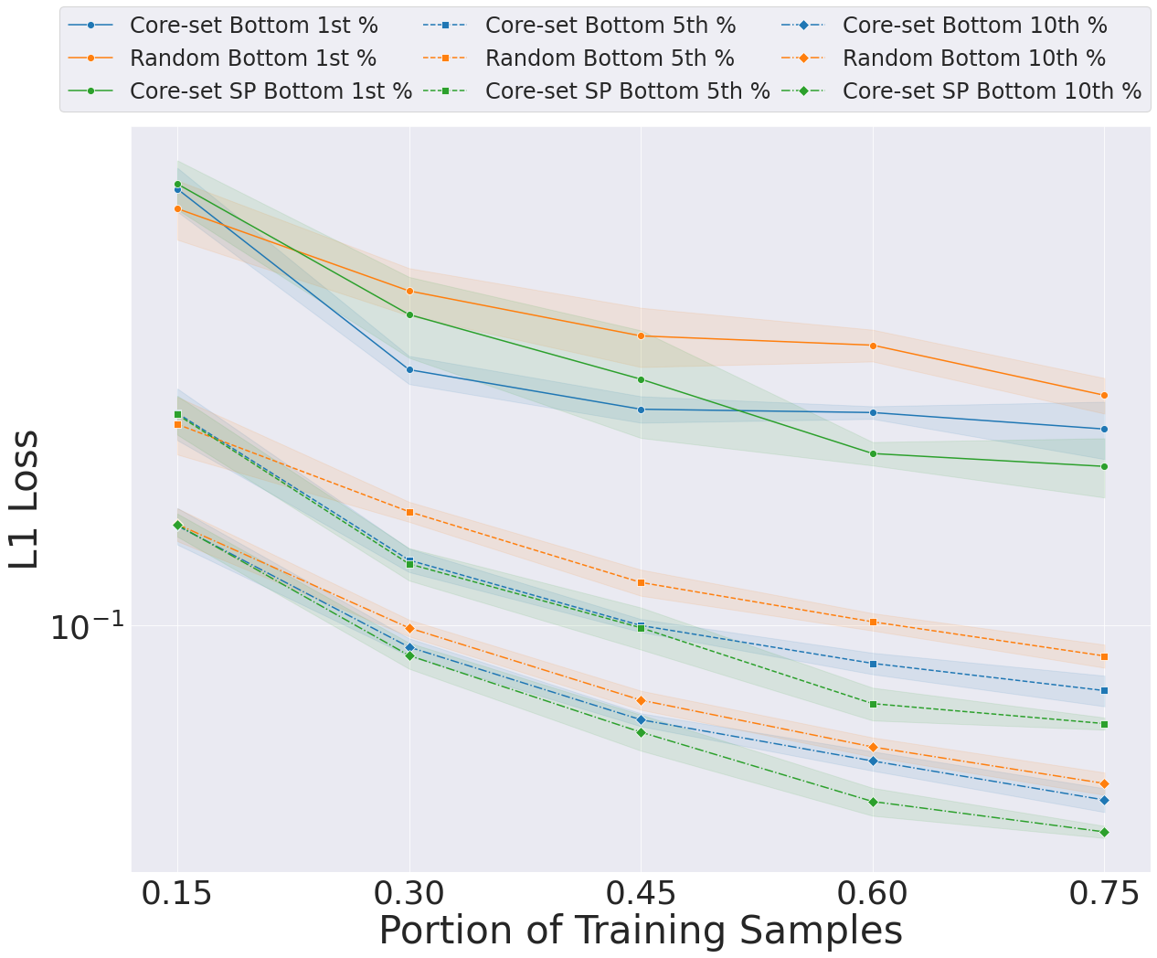
A deterministic, supervised CNNs-based model architecture [5, 15] was used for all experiments. We trained the models with $L_{1}$ -loss function and Adam [16] optimiser with a minibatch size of $32$ and learning rate $0.001$ , and judged their performance by the average $L_{1}$ losses of the bottom 1^st, 5^th and 10^th percentiles. We also plotted the median predictions in Figure 4 and Figure 4 to show that the emulation quality for the better half of the test cases does not vary much with the sampling method. For core-set selection, we solved the k-center problem at virtually no overhead costs using KeOps library [14]. Model outputs were used as the features for core-set, effectively bounding the greatest L1 loss among the samples. Other important hyper-parameters are noted in Table 1. All experiments were run with 4 NVIDIA Tesla T4 GPUs on Google Cloud Platform.

From Figure 4, it is clear that core-set selection outperforms random sampling consistently in reducing the long tail $L_{1}$ losses in all percentiles investigated. Moreover, we needed significantly less data when using core-set selection to achieve similar performance as their random sampling counterpart. Notably, to improve the bottom first percentile of the Halo emulation to a competitive level, a whopping $60\%$ reduction in costs was seen (see Figure 4) using core-set selection. This is highlighted in Figure 4 where the emulator failed to predict part of the signal when it was trained with $10,000$ randomly sampled data, but successfully emulated similar signals using data from core-set.

Furthermore, we recorded marginal, but important improvement in the long tail $L_{1}$ losses when the shrink-and-perturb trick is used in conjunction with the core-set approach, with $\sigma=0.1$ and $\lambda=0.5$ .

4 Conclusions

We investigated how a diversity-based active learning approach, core-set selection, affects the long tail losses in scientific emulations, and how the active learning iterations could be warm started to improve the model performance and save costs. Our experiments show promising results: the long tail losses were significantly reduced without compromising the quality of the better emulations.

5 Broader Impact

On the negative side, designing a good, explainable model architecture to replace the theoretically-grounded scientific simulations could be time-consuming, and a performant model is not necessarily explicable. Besides, modern deep learning is over-dependent on supervised learning, where the performance is in turn reliant on the availability of labelled data.

Our work partially solves the data problem. Using actively sampled, good quality data could improve the general performance of supervised emulators with less data required and thus accelerate scientific research. Moreover, replacing simulators with neural networks trained with actively selected data would significantly reduce computational costs and the adverse environmental impacts that come with heavy computations.

References

Brockherde et al. [2017] Felix Brockherde, Leslie Vogt, Li Li, Mark E Tuckerman, Kieron Burke, and Klaus-Robert Müller. Bypassing the kohn-sham equations with machine learning. Nature communications, 8(1):1–10, 2017.
Kwan et al. [2015] Juliana Kwan, Katrin Heitmann, Salman Habib, Nikhil Padmanabhan, Earl Lawrence, Hal Finkel, Nicholas Frontiere, and Adrian Pope. Cosmic emulation: fast predictions for the galaxy power spectrum. The Astrophysical Journal, 810(1):35, 2015.
Peterson et al. [2017] Jayson L Peterson, KD Humbird, John E Field, Scott T Brandon, Steve H Langer, Ryan C Nora, Brian K Spears, and PT Springer. Zonal flow generation in inertial confinement fusion implosions. Physics of Plasmas, 24(3):032702, 2017.
Rupp et al. [2012] Matthias Rupp, Alexandre Tkatchenko, Klaus-Robert Müller, and O Anatole Von Lilienfeld. Fast and accurate modeling of molecular atomization energies with machine learning. Physical review letters, 108(5):058301, 2012.
Kasim et al. [2021] Muhammad Firmansyah Kasim, D Watson-Parris, L Deaconu, S Oliver, P Hatfield, Dustin H Froula, Gianluca Gregori, M Jarvis, S Khatiwala, J Korenaga, et al. Building high accuracy emulators for scientific simulations with deep neural architecture search. Machine Learning: Science and Technology, 2021.
Sener and Savarese [2017] Ozan Sener and Silvio Savarese. Active learning for convolutional neural networks: A core-set approach. arXiv preprint arXiv:1708.00489, 2017.
Gal et al. [2017] Yarin Gal, Riashat Islam, and Zoubin Ghahramani. Deep bayesian active learning with image data. In International Conference on Machine Learning, pages 1183–1192. PMLR, 2017.
Ash et al. [2019] Jordan T Ash, Chicheng Zhang, Akshay Krishnamurthy, John Langford, and Alekh Agarwal. Deep batch active learning by diverse, uncertain gradient lower bounds. arXiv preprint arXiv:1906.03671, 2019.
Kirsch et al. [2019] Andreas Kirsch, Joost Van Amersfoort, and Yarin Gal. Batchbald: Efficient and diverse batch acquisition for deep bayesian active learning. Advances in neural information processing systems, 32:7026–7037, 2019.
Regan et al. [2013] SP Regan, R Epstein, BA Hammel, LJ Suter, HA Scott, MA Barrios, DK Bradley, DA Callahan, C Cerjan, GW Collins, et al. Hot-spot mix in ignition-scale inertial confinement fusion targets. Physical review letters, 111(4):045001, 2013.
Ciricosta et al. [2017] Orlando Ciricosta, H Scott, P Durey, BA Hammel, R Epstein, TR Preston, SP Regan, SM Vinko, NC Woolsey, and JS Wark. Simultaneous diagnosis of radial profiles and mix in nif ignition-scale implosions via x-ray spectroscopy. Physics of Plasmas, 24(11):112703, 2017.
Wake et al. [2011] David A Wake, Katherine E Whitaker, Ivo Labbé, Pieter G Van Dokkum, Marijn Franx, Ryan Quadri, Gabriel Brammer, Mariska Kriek, Britt F Lundgren, Danilo Marchesini, et al. Galaxy clustering in the newfirm medium band survey: the relationship between stellar mass and dark matter halo mass at 1< z< 2. The Astrophysical Journal, 728(1):46, 2011.
Ash and Adams [2019] Jordan T Ash and Ryan P Adams. On warm-starting neural network training. arXiv preprint arXiv:1910.08475, 2019.
Charlier et al. [2021] Benjamin Charlier, Jean Feydy, Joan Alexis Glaunès, François-David Collin, and Ghislain Durif. Kernel operations on the gpu, with autodiff, without memory overflows. Journal of Machine Learning Research, 22(74):1–6, 2021. URL http://jmlr.org/papers/v22/20-275.html.
He et al. [2016] Kaiming He, Xiangyu Zhang, Shaoqing Ren, and Jian Sun. Deep residual learning for image recognition. In Proceedings of the IEEE conference on computer vision and pattern recognition, pages 770–778, 2016.
Kingma and Ba [2014] Diederik P Kingma and Jimmy Ba. Adam: A method for stochastic optimization. arXiv preprint arXiv:1412.6980, 2014.

Appendix A Future Expected Loss

The future expected loss can be upper bounded by the summation of three terms, namely generalisation error, training error and core-set loss. In an expressive model such as CNNs, the generalisation and training errors can be assumed to be negligible, thus simplifying the upper bound to just the core-set loss.

\displaystyle E_{\mathbf{x},\mathbf{y}\sim p_{z}}\left[l(\mathbf{x},\mathbf{y};A_{\mathbf{s}})\right]

\displaystyle\leq\begin{aligned} &\underbrace{\Bigl|E_{\mathbf{x},\mathbf{y}\sim p_{z}}\left[l(\mathbf{x},\mathbf{y};A_{\mathbf{s}})\right]-\frac{1}{n}\sum_{i=1}^{n}l(\mathbf{x}_{i},\mathbf{y}_{i};A_{\mathbf{s}})\Bigr|}_{\text{Generalisation Error}}\\ &+\underbrace{\frac{1}{|\mathbf{s}|}\sum_{j\in\mathbf{s}}l(\mathbf{x}_{j},\mathbf{y}_{j};A_{\mathbf{s}})}_{\text{Training Error}}\\ &+\underbrace{\Bigl|\frac{1}{n}\sum_{i=1}^{n}l(\mathbf{x}_{i},\mathbf{y}_{i};A_{\mathbf{s}})-\frac{1}{|\mathbf{s}|}\sum_{j\in\mathbf{s}}l(\mathbf{x}_{j},\mathbf{y}_{j};A_{\mathbf{s}})\Bigr|}_{\text{Core-set Loss}}\end{aligned}

Appendix B Proof for Lemma 1

Consider two vectors $\mathbf{x}^{d}$ and $\mathbf{\tilde{x}}^{d}$ that correspond to inputs $\mathbf{x}$ and $\mathbf{\tilde{x}}$ at layer $d$ of a neural net respectively. First, for any convolutional or fully connected layer, for each node $j$ in layer $d$ , we can write $\mathbf{x}_{j}^{d}=\sum_{i}w^{d}_{i,j}\mathbf{x}_{i}^{d-1}$ . Now, assuming $\sum_{i}|w_{i,j}|\leq\alpha$ for all $i,\>j,\>d$ , we can write, for any convolutional or fully connected layer:

||\mathbf{x}^{d}-\mathbf{\tilde{x}}^{d}||_{q}\leq\alpha||\mathbf{x}^{d-1}-\mathbf{\tilde{x}}^{d-1}||_{q}

(4)

for any real $q\geq 1$ .

For ReLU, we note that $|a-b|\geq|\max{(0,a)}-\max{(0,b)}|$ , and as such we can state:

||\mathbf{x}^{r}-\mathbf{\tilde{x}}^{r}||_{q}\leq||\mathbf{x}^{r-1}-\mathbf{\tilde{x}}^{r-1}||_{q}

(5)

where the superscripts $r-1$ and $r$ indicate before and after the ReLU activation function respectively.

Combining Equation 4 and Equation 5, for ReLU-activated neural networks with $\eta_{c}$ convolutional layers and $\eta_{fc}$ fully connected layers, we get

||CNN(\mathbf{x};\mathbf{w})-CNN(\mathbf{\tilde{x}};\mathbf{w})||_{q}\leq\alpha^{\eta_{c}+\eta_{fc}}||\mathbf{x}-\mathbf{\tilde{x}}||_{q}

Finally, using reverse triangle inequality, we obtain

|l(\mathbf{x},\mathbf{y};\mathbf{w})-l(\mathbf{\tilde{x}},\mathbf{y};\mathbf{w})|=|||CNN(\mathbf{x};\mathbf{w})-\mathbf{y}||_{q}-||CNN(\mathbf{\tilde{x}};\mathbf{w})-\mathbf{y}||_{q}|\leq||CNN(\mathbf{x};\mathbf{w})-CNN(\mathbf{\tilde{x}};\mathbf{w})||_{q}

hence finishing the proof.

Appendix C Proof for Theorem 1

We note that for two probability density functions $p$ and $p^{*}$ defined over the space $\mathcal{Y}$ , the following is always true:

\int p\,dy\leq\int p^{*}\,dy+\int|p-p^{*}|\,dy

(6)

Then, we bound $E_{\mathbf{y}\sim\eta({\mathbf{x}_{i}})}\left[l(\mathbf{x}_{i},\mathbf{y};A_{\mathbf{s}})\right]$ by using Equation 6:

	$\displaystyle E_{\mathbf{y}\sim\eta({\mathbf{x}_{i}})}\left[l(\mathbf{x}_{i},\mathbf{y};A_{\mathbf{s}})\right]$	$\displaystyle=\int p_{\mathbf{y}\sim\eta(\mathbf{x}_{i})}(\mathbf{y})\left[l(\mathbf{x}_{i},\mathbf{y};A_{\mathbf{s}})\right]\,d\mathbf{y}$
		$\displaystyle\leq\begin{aligned} &\int p_{\mathbf{y}\sim\eta(\mathbf{x}_{j})}(\mathbf{y})\left[l(\mathbf{x}_{i},\mathbf{y};A_{\mathbf{s}})\right]\,d\mathbf{y}\\ &+\int\|p_{\mathbf{y}\sim\eta(\mathbf{x}_{i})}(\mathbf{y})-p_{\mathbf{y}\sim\eta(\mathbf{x}_{j})}(\mathbf{y})\|\left[l(\mathbf{x}_{i},\mathbf{y};A_{\mathbf{s}})\right]\,d\mathbf{y}\end{aligned}$
		$\displaystyle\leq\int p_{\mathbf{y}\sim\eta(\mathbf{x}_{j})}(\mathbf{y})\left[l(\mathbf{x}_{i},\mathbf{y};A_{\mathbf{s}})\right]\,d\mathbf{y}+\delta\lambda^{\eta}L\int d\mathbf{y}$
		$\displaystyle=\int p_{\mathbf{y}\sim\eta(\mathbf{x}_{j})}(\mathbf{y})\left[l(\mathbf{x}_{i},\mathbf{y};A_{\mathbf{s}})\right]\,d\mathbf{y}+\delta\lambda^{\eta}LV$

where $\mathbf{x}_{j}$ for $j\in[m]$ are labelled training data. Then, recall the assumption that the trained networks would fit perfectly to the training samples and using Lemma 1, we get

	$\displaystyle\int p_{\mathbf{y}\sim\eta(\mathbf{x}_{j})}(\mathbf{y})\left[l(\mathbf{x}_{i},\mathbf{y};A_{\mathbf{s}})\right]\,d\mathbf{y}$	$\displaystyle=\begin{aligned} &\int p_{\mathbf{y}\sim\eta(\mathbf{x}_{j})}(\mathbf{y})\left[l(\mathbf{x}_{i},\mathbf{y};A_{\mathbf{s}})-l(\mathbf{x_{j}},\mathbf{y};A_{\mathbf{s}})\right]\,d\mathbf{y}\\ &+\int p_{\mathbf{y}\sim\eta(\mathbf{x}_{j})}(\mathbf{y})\left[l(\mathbf{x_{j}},\mathbf{y};A_{\mathbf{s}})\right]\,d\mathbf{y}\end{aligned}$
		$\displaystyle\leq\delta\lambda^{l}$

which gives us

E_{\mathbf{y}\sim\eta({\mathbf{x}_{i}})}\left[l(\mathbf{x}_{i},\mathbf{y};A_{\mathbf{s}})\right]\leq\delta\left[\lambda^{l}+\lambda^{\eta}LV\right]

Finally, using Hoeffding’s Bound, we conclude that with a probability of at least $1-\gamma$ , we get an upper bound for the core-set loss,

\Bigl|\frac{1}{n}\sum_{i\in[n]}l(\mathbf{x}_{i},\mathbf{y}_{i};A_{\mathbf{s}})-\frac{1}{|\mathbf{s}|}\sum_{j\in\mathbf{s}}l(\mathbf{x}_{j},\mathbf{y}_{j};A_{\mathbf{s}})\Bigr|\leq\delta\left[\lambda^{l}+\lambda^{\eta}LV\right]+\sqrt{\frac{L^{2}\log(1/\gamma)}{2n}}