ExoMol molecular line lists – XLIII: Rovibronic transitions corresponding to the close-lying X and A states of NaOYYYYExoMol molecular line lists – XLIII: Rovibronic transitions corresponding to the close-lying X and A states of NaO–References
Abstract
The sodium monoxide radical (NaO) is observed in night glow in the Earth’s mesosphere and likely has astronomical importance. This study concerns the optical transitions within the ground X state and to the very low-lying ( cm-1) excited A state. A line list consisting of rovibronic term values, allowed electric dipole transitions, Einstein coefficients, and partition functions for varying temperature are produced due to a variational solution of the coupled-channel Schrödinger equations using the program Duo. MRCI ab initio calculations characterising the potential energy curves of the both states, spin-orbit and -uncoupling non-adiabatic matrix elements, as well as permanent and transition dipole moments were integral in formation of the final deperturbation model. Ab initio potential energy curves are represented in the analytical Extended-Morse-Oscillator form and refined, along with the spin-orbit and -uncoupling functions, by least-squares fitting to the available spectroscopic data. The input experimental data consisted of pure rotational transitions within the fine structure components of the X state for vibrational levels as well as the rovibronic A X transitions, both with limited coverage over rotational excitation. The lack of data detailing the vibrational structure of the X and A states prompts a request for further experimental study of higher excited levels which would provide a robust spectroscopic model. The NaO NaOUCMe line list is available via www.exomol.com and the CDS database.
Keywords:
keyword1 – keyword2 – keyword31 Introduction
Air-glow, sometimes referred to as night-glow, was first reported by Slipher 1929 and has been identified as the emission of Na D-lines. It is proposed that these lines arise from the Chapman mechanism (Chapman 1939; Sarkhel et al. 2010; Plane et al. 2012) with some modifications suggested in light of modern measurements (Slanger et al. 2005; Sarkhel et al. 2010), as given by
| (1) |
| (2) | ||||
| (3) |
| (4) |
where are the temperature-dependent rate constants, is the branching ratio, and are the D-line transition energies.
This mechanism suggests that Na atoms, which are assumed to be ablated from meteors, react with O3 in the atmosphere to form NaO, re-reacting with O atom to reform Na. Long lasting visible meteor trails have been attributed to the production of electronically excited Na by in the said reaction chain (Kolb & Elgin 1976; Joo et al. 1999). In the Chapman mechanism, the rate limiting reaction is the formation of NaO, see Eq. (1). As this reaction takes place in the mesosphere, the variation of mesospheric ozone concentration affects Na air-glow intensity. As altitude profiles of ozone are available, ozone concentration variation can be used for deeper study into Sodium air-glow and subsequently NaO. (Plane 2003; Sarkhel et al. 2010).
The experimental spectroscopic data related to optical transitions of the gas-phase NaO molecules is very sparse. Yamada et al. 1989 provide comprehensive microwave data on the pure rotational transitions of the ground X electronic state for the lowest vibrational levels. However, no experimental data on ro-vibrational transitions are available, and hence, the separations between vibrational levels are not yet experimentally determined. Some information is available on the B X emission spectrum, however this is minimal, unassigned with no characterisation of the B state (Pfeifer & Gole 1984; Pugh et al. 1996), which sometimes is assigned as C state (Langhoff et al. 1991). The only experimental observation of the lowest excited A state is due to Joo et al. 1999 who could assign a handful of the low rotational levels belonging to the rovibronic A X transitions.
The electronic structure of NaO demonstrates pronounced ionic inter-atomic bond leading to large permanent dipoles as well as the close-lying ground X and first excited A state converging to different dissociation thresholds. The low excitation energy of the A state means that its spin-allowed A–X electronic transition lies in the infrared, largely in the 3 to 5 m region. From the theoretical viewpoint, the A and X states are expected to be strongly coupled to each other due to spin-orbit and electronic-rotational intramolecular perturbations. Ab initio potential energy curves (PECs) and permanent dipole moments are available for both lowest electronic states (Buenker & Liebermann 2009; Langhoff et al. 1991; Soldán et al. 1999). However, the corresponding non-adiabatic coupling matrix elements are not known so far.
In this paper we present new ab initio PECs for both X and A states of NaO accompanied by spin-orbit and -uncoupling non-adiabatic matrix elements which we tune to the limited available spectroscopic data. Finally, a rovibronic line list for NaO is simulated to be suitable for modeling spectra up to temperature 2500 K. This line list is constructed as part of the ExoMol project (Tennyson & Yurchenko 2012). We note that a previous ExoMol line list for CaO (Yurchenko et al. 2016b), constructed using similar methodology to that employed here, was used by Berezhnoy et al. 2018 to assign a spectrum of CaO in the wake of the Beneshov bolide at the height of 29 km above the Earth’s surface.
2 Method
2.1 Ab initio electronic structure calculation
The initial set of required potential energy curves (PECs), permanent and transition dipole moments for the ground X and near-lying excited A states of NaO were obtained in the framework of ab initio electronic structure calculations which were accompanied by the evaluation of the relevant non-adiabatic matrix elements for the spin-orbit and Coriolis (electron-rotational) coupling. Scalar relativistic effects are introduced by means of the second-order Douglas-Kroll Hamiltonian (Reiher & Wolf 2004). All calculations were performed in the range of internuclear distance Å using the MOLPRO program suite (Werner et al. 2010).
For both Na and O atoms, aug-cc-pVQZ all electrons basis sets was used. The optimized molecular orbitals (MO’s) were generated using the state-averaged self-consistent field (SA-CASSCF) method (Werner & Knowles 1985), taking the lowest doublet (1-3), (1), (1), and (1) states with equal weights. Internally-contracted multi-reference configuration interaction (MR-CISD) calculations (Knowles & Werner 1992) followed, in which impact of higher excitation on the correlation energy was taken into account implicitly using the Davidson correction (Langhoff & Davidson 1974). For both SA-CASSCF and MR-CISD steps the active space consisted of , and orbitals corresponding to the point group symmetry , while the lowest two orbitals were kept to be doubly occupied. The full counterpoise correction (Boys & Bernardi 1970) was accounted for each state individually with the residual size-consistency error eliminated at Å.
Both permanent and transition dipole moments as well as non-adiabatic -uncoupling matrix element were computed using the MR-CISD wave functions. The same wave functions and the full Breit-Pauli operator were used to compute the SOCs (Berning et al. 2000).
2.2 Fitting procedure
The adiabatic PECs ab initio calculated above in Sec. 2.1 were combined with the relevant spin-orbit coupling (SOC) and -uncoupling functions in order to evaluate non-adiabatic rovibronic term values and corresponding multi-channel wavefunctions for the mutually perturbed X and A states of NaO. However, the pure ab initio estimates are a priori and are not accurate enough to predict the rovibronic energy with the spectroscopic accuracy required. For better agreement between predicted and observed transitions, PECs and coupling curves are refined by making constrained adjustments to the parameters which describe them (see below). This is done by a least-squares fitting to experimental data and is performed in Duo, an open-source Fortran 2009 program which provides variational solutions to the coupled rovibronic Schrodinger equations for a general open-shell diatomic molecule (Yurchenko et al. 2016a).
The input set of the experimental data taken from (Yamada et al. 1989) consisted of pure rotational transition frequencies (with and ) within up to . Joo et al. 1999 provided rovibronic frequencies for the A – X band with up to together with relative absorption intensities. Joo et al. also observed the band suggesting an A state vibrational spacing of 498.9 cm-1. This spacing was included in the present fit using an artificial line for .
The ab initio point-wise PECs of both states treated were approximated using the fully analytical Extended Morse Oscillator (EMO) form (Lee et al. 1999; Yurchenko et al. 2016a; Le Roy 2017):
| (5) |
where is the electronic term, is the dissociation energy and is the equilibrium distance. In contrast to the conventional Morse potential, the -dependent exponent coefficient in Eq. (5) is defined as the polynomial series
| (6) |
with respect to the reduced coordinate
| (7) |
which was first introduced by Šurkus et al. 1984.
At the first step, the EMO potentials (5) were least-squares fit to the original ab initio PECs in Python. The electronic energy of the ground state was fixed to zero, and both PECs were fit to fourth order in the polynomial expansion (6). The parameter in Eq.(7) was fixed to 6 and 4 for the ground and excited state, respectively.
At the second step, the resulting ab initio EMO PECs were refined by adjusting to the experimental transition frequencies (Joo et al. 1999; Yamada et al. 1989) where only (X, A), (A), (X) and (A) fitting parameters were varied. Furthermore, both diagonal, , and off-diagonal, , spin-orbit coupling (SOCs) functions as well as -uncoupling function, , between A and X states were also fitted simultaneously with the trial EMO PECs above. This was particularly done using the facility in Duo to adjust curves using a morphing function, :
| (8) |
where C is the coupling curve in question. are the original ab initio point-wise functions interpolated by ordinary cubic splines with so-called natural boundary conditions. The morphing function, , in Eq.(8), is tacitly assumed to be an analytical function of the internuclear distance , and it was modelled by the following linear function
| (9) |
of the Šurkus-like variable, , (see Eq. (7)), where the equilibrium distance is substituted for the fixed parameter Å . The parameter and are also fixed for all morphing functions while only parameter is kept to be variable.
Morphing (Eq: 8) was used as it avoids the need for an analytical representation of the ab initio point-wise coupling curves by changing their original shapes directly. This approach is, however, not normally applied for PECs for the reason of difficulty to control the equilibrium parameter , which is a value of interest not explicitly derivable from this morphing form.
3 Results and Discussion
3.1 Potential energy curves, spin-orbit and -uncoupling matrix elements
The resulting ab initio adiabatic PECs obtained for the X- and A-states of NaO are depicted on Fig. 1 together with their empirical (adjusted) counterparts. The fitted parameters of the EMO potentials (Eq. (5)) for the both states treated are collected in Table 2. The corresponding ab initio diagonal spin-orbit function, , of the ground X-state as well as the off-diagonal SOC, , and the -uncoupling, , functions are shown in Fig. 2. The relevant morphing parameters for these functions are given in Table 2.
The fitted EMO PECs and coupling functions reproduce the input experimental data with an overall root-mean-squares (RMS) error of . This RMS is deceptively large due to the pronounced discrepancy of the A artificial line, skewing the mean RMS, see Table 1. Indeed, for the ground X state, there is agreement with the experiment on order of cm-1and for the case there is agreement on order cm-1.
The ab initio function obeys Van Vleck’s hypothesis (Mulliken & Christy 1931) of pure precession in the interval Å :
| (10) |
where the total electronic angular momentum of molecule is equal to 1 while its projection on the internuclear axis is zero. Moreover, the relationship
| (11) |
between diagonal and off-diagonal spin-orbit functions is valid as well.
The ab initio SO splitting of the ground X-state is found to be close to the empirical value determined by Yamada et al. 1989 (see Table 3). The reliability of the ab initio off-diagonal spin-orbit -uncoupling functions is indirectly confirmed by a good agreement of the -doubling constants (, ) empirically obtained for the regular perturbed levels of the ground state by Yamada et al. 1989 with their theoretical counterparts roughly estimated for the lowest vibrational levels, , according to the relations (Lefebvre-Brion & Field 2004; Pazyuk et al. 1994):
| (12) |
| (13) |
where , is the reduced molecular mass, is the difference of PECs, while are the vibrational wavefunctions of the ground state.


| 0 | 0.002664 | 0.022501 |
|---|---|---|
| 1 | 0.002846 | 0.679901a |
| 2 | 0.002758 | |
| 3 | 0.017115 | |
| Ave. | 0.006345 | 0.351201 |
a: artificial line, see Sec. 2.2.
| PEC Parameterisation | ||
|---|---|---|
| EMO Param. | X | A |
| 0 | 2029.147a | |
| 2.05189a | 1.96723a | |
| 21735.7 | 35496.4 | |
| 6 | 4 | |
| 2 | 2 | |
| 4 | 4 | |
| 1.50708327083484a | 0.989061691136872a | |
| -0.04809897091909 | 0.181504940347642 | |
| 0.16743487156786 | 0.424100841906937 | |
| -0.95627676523677 | -2.926458322108940 | |
| 1.16624139895144 | 2.522897112151440 | |
| parameters used for morphed coupling functionsc | ||
| Function | ||
| 1.0098 | ||
| 0.6277 | ||
| -0.7455 | ||


| Parameter | Empirical | Ab initio |
|---|---|---|
| -107 | -120 | |
| p | +0.044 | +0.04 |
| q | +0.0003 | +0.0003 |
3.2 Permanent and Transition Dipole Moments
The ab initio permanent dipole moments , calculated for the X and A states of the NaO molecule are given in Fig. 3 together with the corresponding A–X transition dipole moment . The present dipole moments are in a good agreement with their previous theoretical counterparts computed by Langhoff et al. 1991.
According to the expected ion-pair character of the interatomic bond, the permanent dipole moments of both A and X states are rapidly increasing linear functions of while the corresponding A–X electronic transition dipole moment is very small, but not negligible (see Fig. 3). The maximal values of the present A–X transition moment are about 0.1-0.15 a.u. which agree well with the estimate D given in Joo et al. 1999. At Å, the ground state permanent dipole decreases due to the avoided crossing effect with the excited state. An even more abrupt drop in the permanent dipole is observed for the A-state but at larger internuclear distances, presumably also due to an avoided crossing.
O’Hare & Wahl 1972 give an equilibrium dipole moment for the X state of 8.71 D which was adopted by the JPL Molecular Spectroscopy Database (Pickett et al. 1998) to provide transition intensities. Our ab initio equilibrium value is D, while the vibrationally averaged dipole moment extracted from the Duo the matrix element is 8.44 D, which is very similar to the equilibrium dipole moment. Our results suggest that JPL predicted transitions are slightly (about 6%) too strong.

3.3 Partition Function
The temperature dependent partition function for NaO molecule was calculated as the sum:
| (14) |
where is the total degeneracy of the state, is the nuclear statistical weight factor, and is the Boltzmann constant. As sums over , the value of at some depends on the value of used in the sum. To ensure completeness of the line list, it is a requirement that, up to a given temperature, in the case of this study, 2500 K, the value of converges with . As shown in Fig. 4, use converges at K.

The JPL database provides partition function values up to =300 K. Barklem & Collet 2016 provide numerical values for the partition functions of NaO up to 10 000 K which we multiply by four to account for different treatments of the Na nuclear spin degeneracy; we (and JPL) include (which is appropriate for ) into , while Barklem & Collet 2016 does not. A comparison between these partition functions is given in Fig. 5. The JPL values agree well with ours (see Table 4), with level of agreement decreasing as temperature goes up which likely due to a lack of higher vibrational levels contribution in JPL partition sum. However, there is poor coincidence with Barklem & Collet 2016 at low temperature with agreement improving for higher temperature. The reason for the low temperature disagreement between Barklem & Collet 2016 and the results of JPL and our own is unclear but we believe our values are correct in this region. It should be noted that the data from Barklem & Collet 2016 is based on calculated rather than experimental molecular constants taken from Huber & Herzberg 1979.


| T / K | Q | Q | /% |
|---|---|---|---|
| 300 | 7027.4727 | 6633.1886 | 5.61 |
| 225 | 4694.9814 | 4491.5223 | 4.33 |
| 150 | 2734.0243 | 2645.0047 | 3.26 |
| 75 | 1134.4648 | 1109.3245 | 2.22 |
| 37.5 | 518.8865 | 516.1226 | 0.53 |
| 18.75 | 262.9106 | 262.9886 | -0.030 |
| 9.375 | 139.2536 | 139.3226 | -0.050 |
| State | X | A | ||
|---|---|---|---|---|
| Case | , | , | all and levels | |
| Uncertainty | 0.003 | 20-40 | 10-30 | |
3.4 Final line list and absorption spectra simulation
The Duo package was used to produce a NaO line list which we call NaOUCMe. This line list is given in ExoMol format (Tennyson et al. 2014; Tennyson et al. 2020) as "*.states" file containing term values for the lowest 36 120 rovibronic levels of the complex up to and and a "*.trans" file consisting of the corresponding Einstein coefficients and frequencies for 4 726 137 dipole-allowed , and transitions. In line with the updated ExoMol standard (Tennyson et al. 2020), the "*.states" files also provide approximate uncertainties for the energies which allow the accuracy with which we predict each transition to be estimated. For fitted regions, we recommend transition uncertainties equal to those in Table 1. For the ground electronic state, for the case where and , an uncertainty of is recommended. Typically, energy level uncertainties scale with quadratically and the following functional form for is recommended: . For all other (extrapolated) cases in the X state, the ab initio vibrational uncertainty takes precedence at 20-40 cm-1.
The vibrational spacing between the and states were fit to a satisfactory level of agreement (artificial line from sec. 2.2). However, it is recommended that this line list only be used for high resolution observational studies at long wavelengths spectral range covering pure rotational transitions. Overall energy level uncertainties are summarised in Table 5.
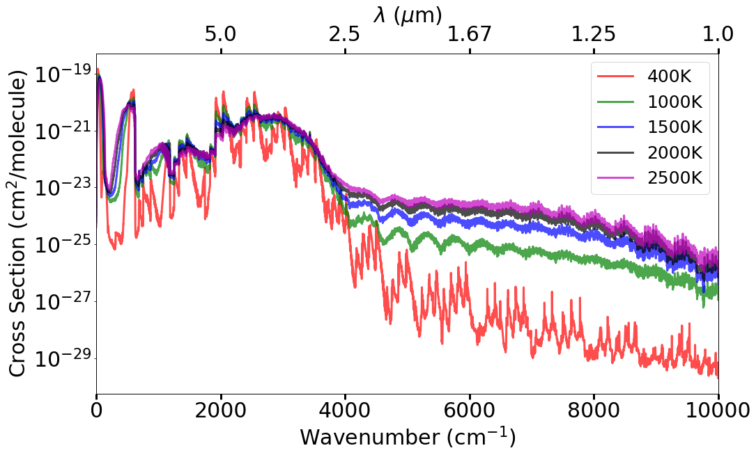
Samples from the "*.states" and "*.trans" files are given in Tables 6 and 7. These were processed in ExoCross (Yurchenko et al. 2018) to produce Fig. 6, an absolute absorption spectrum for the region studied by Joo et al. 1999, and Fig. 7, the absorbance cross section for NaO as a function of temperature computed at a resolution of 1 cm-1 with a half-width at half-maximum (HWHM) of 1 cm-1.
| NN | Energy | gtot | uncertainty | lifetime | Landé | e/f | State | ||||||
|---|---|---|---|---|---|---|---|---|---|---|---|---|---|
| 1 | 118.305521 | 8 | 0.5 | 0.003000 | 5.1528E+03 | 0.001493 | + | e | X2Pi | 0 | 1 | -0.5 | 0.5 |
| 2 | 704.551592 | 8 | 0.5 | 30.000000 | 2.8981E+00 | 0.001932 | + | e | X2Pi | 1 | 1 | -0.5 | 0.5 |
| 3 | 1282.294758 | 8 | 0.5 | 30.000000 | 1.4807E+00 | 0.002994 | + | e | X2Pi | 2 | 1 | -0.5 | 0.5 |
| 4 | 1850.69127 | 8 | 0.5 | 30.000000 | 1.0028E+00 | 0.012246 | + | e | X2Pi | 3 | 1 | -0.5 | 0.5 |
| 5 | 2045.653545 | 8 | 0.5 | 20.000000 | 1.0894E-01 | 1.988261 | + | e | A2Sigma | 0 | 0 | 0.5 | 0.5 |
| 6 | 2409.940124 | 8 | 0.5 | 30.000000 | 6.5698E-01 | 0.041505 | + | e | X2Pi | 4 | 1 | -0.5 | 0.5 |
| 7 | 2544.609918 | 8 | 0.5 | 20.000000 | 6.4721E-02 | 1.957978 | + | e | A2Sigma | 1 | 0 | 0.5 | 0.5 |
| 8 | 2960.425378 | 8 | 0.5 | 30.000000 | 3.7063E-01 | 0.112844 | + | e | X2Pi | 5 | 1 | -0.5 | 0.5 |
| 9 | 3042.140902 | 8 | 0.5 | 20.000000 | 4.9272E-02 | 1.887345 | + | e | A2Sigma | 2 | 0 | 0.5 | 0.5 |
| 10 | 3501.549396 | 8 | 0.5 | 30.000000 | 1.4379E-01 | 0.388061 | + | e | X2Pi | 6 | 1 | -0.5 | 0.5 |
NN: State counting number,
Energy: State energy in cm-1,
gtot: Total degeneracy of the state,
: Angular momentum quantum number,
uncertainty: Energy level uncertainty in cm-1,
lifetime: Lifetime of the state in seconds,
Landé: Landé factor (Semenov
et al. 2017),
: Parity,
e/f: Rotationless parity,
State: Electronic state, X2Pi or A2Sigma+
: Vibrational quantum number,
: Projection of electronic angular momentum,
: Projection of electronic spin,
: (Projection of total electron angular momentum).
| n | n | A | |
|---|---|---|---|
| 2097 | 2007 | 7.7832E-17 | 0.001009 |
| 843 | 933 | 2.4392E-16 | 0.001035 |
| 1799 | 1889 | 9.3118E-17 | 0.001043 |
| 1883 | 1793 | 9.4292E-17 | 0.001055 |
| 1219 | 1309 | 1.6125E-16 | 0.001066 |
| 3848 | 3758 | 2.7618E-17 | 0.001137 |
| 1520 | 1430 | 1.7928E-16 | 0.001148 |
| 1595 | 1685 | 1.3851E-16 | 0.001153 |
| 3146 | 3056 | 4.9277E-17 | 0.001177 |
| 1688 | 1598 | 1.5019E-16 | 0.001179 |
| 766 | 676 | 5.6326E-16 | 0.001185 |
n: Lower state counting number
n: Upper state counting number
A: Einstein A-coefficient in s-1
: Transition wavenumber in cm-1
3.5 Comparison with the experimental X A spectra
The experimental A X absorption bands were observed by Joo et al. 1999 but their measurements were only sensitive in the very narrow spectral regions: 2015–2095 cm-1 and 2646–2697 cm-1. The lines in these regions were assigned to the and bands respectively. An absolute intensity absorption spectrum was calculated as a stick spectrum to compare to this, see Fig. 6. The calculated absorption lines result in a line profile significantly broader than those visible from measurements of Joo et al. 1999. The observed spectrum (relative intensities) has been scaled by matching the intensity of the strongest line [A X ] from experiment to that of its conjugate calculated line; it can be seen that the observed transitions lie on the tail end, -branch of the calculated absorption spectrum with a matching downward slope.
We note that Joo et al. 1999 used their measurements to determine the vibronic term value for the A(0)–X(0) band, (A), of 1992.905 cm-1. Using approximate zero-point energies (ZPEs) generated by Duo, and shows that our from our deperturbation model is 1982.3 cm-1, which is less than that of Joo et al. 1999 by 10 cm-1. An attempt was made to reproduce the experimental (A) value above by manually adjusting (A) and refitting. However, this results in significantly worse fits in the transitions (around an order of magnitude) without improving agreement of (A) with experiment.

4 Conclusions
An optical line list called NaOUCMe is presented for the alkali monoxide radical, NaO covering transitions in the 0–10000 cm-1 energy range up to and with applicability up to the equilibrium temperature K. The experimental lines for pure rotational transitions in the ground electronic state (Yamada et al. 1989) and rovibronic A X transitions (Joo et al. 1999) were used to refine the deperturbation model applied. An average RMS of cm-1 was achieved for the X state rotational transitions and for the A X transitions, with RMS for the A X transitions and RMS for the A A artificial line (see sec. 2.2). Uncertainties of the reproduced and predicted lines rapidly increase as the vibrational and rotational quantum numbers increase for both electronic states, and, hence, further experimental data on higher excited transitions is required to create a more robust line list.
The success of the CaO line list (Yurchenko et al. 2016c) in a spectrum assignment at 29 km above the Earth’s surface by Berezhnoy et al. 2018 is indicative of potential importance of s-block metal monoxides like NaO. NaO similarly is a molecule that can be studied in a terrestrial environment at approximately 90 km above the Earth’s surface (Slanger et al. 2005) and has been recently studied as a transient species in airglow by Sarkhel et al. 2009; Sarkhel et al. 2010 and Plane et al. 2012. As such, we strongly encourage further experimental study into NaO for refinement of the spectroscopic model and production of a higher accurate line list.
Acknowledgements
We thank Dr. A. A. Berezhnoy for bringing the problem to our attention and Prof. I. A. Osterman for taking part in the preliminary ab initio calculations. This work was supported by ERC Advanced Investigator Project 883830 and by UK STFC under grant ST/R000476/1. A.V.S. is grateful for the support by the Russian Science Foundation (RSF), Grant No.18-13-00269.
Data Availability
The Duo model input file and calculated partition function file given as a supplementary materials to this article. The NaO NaOUCMe states and transition files of can be downloaded from www.exomol.com and the CDS data centre cdsarc.u-strasbg.fr. The open access programs ExoCross and Duo are available from github.com/exomol.
References
- Barklem & Collet (2016) Barklem P. S., Collet R., 2016, A&A, 588, A96
- Berezhnoy et al. (2018) Berezhnoy A. A., Borovicka J., Santos J., Rivas-Silva J. F., Sandoval L., Stolyarov A. V., Palma A., 2018, Planet Space Sci., 151, 27
- Berning et al. (2000) Berning A., Schweizer M., Werner H.-J., Knowles P. J., P. P., 2000, Mol. Phys., 98, 1823
- Boys & Bernardi (1970) Boys S. F., Bernardi F., 1970, Mol. Phys., 19, 553
- Buenker & Liebermann (2009) Buenker R. J., Liebermann H.-P., 2009, J. Chem. Phys., 131, 114107
- Chapman (1939) Chapman S., 1939, ApJ, 90, 309–316
- Huber & Herzberg (1979) Huber K. P., Herzberg G., 1979, Molecular Spectra and Molecular Structure IV. Constants of Diatomic Molecules. Van Nostrand Reinhold Company, New York, doi:10.1007/978-1-4757-0961-2, https://doi.org/10.1007/978-1-4757-0961-2
- Joo et al. (1999) Joo S., Worsnop D. R., Kolb C. E., Kim S. K., Herschbach D. R., 1999, J. Phys. Chem. A, 103, 3193
- Knowles & Werner (1992) Knowles P. J., Werner H.-J., 1992, Theoretical Chemistry Accounts, 84, 95
- Kolb & Elgin (1976) Kolb C. E., Elgin J. B., 1976, Nature, 263, 488–490
- Langhoff & Davidson (1974) Langhoff S. R., Davidson E. R., 1974, Int. J. Quant. Chem., 8, 61
- Langhoff et al. (1991) Langhoff S. R., Partridge H., Bauschlicher C. W., 1991, Chem. Phys., 153, 1–12
- Le Roy (2017) Le Roy R. J., 2017, J. Quant. Spectrosc. Radiat. Transf., 186, 179
- Lee et al. (1999) Lee E. G., Seto J. Y., Hirao T., Bernath P. F., Le Roy R. J., 1999, J. Mol. Spectrosc., 194, 197
- Lefebvre-Brion & Field (2004) Lefebvre-Brion H., Field R. W., 2004, The Spectra and Dynamics of Diatomic Molecules: Revised and Enlarged Edition. Academic Press
- Mulliken & Christy (1931) Mulliken R. S., Christy A., 1931, Phys. Rev., 38, 87
- O’Hare & Wahl (1972) O’Hare P. A. G., Wahl A. C., 1972, J. Chem. Phys., 56, 4516–4525
- Pazyuk et al. (1994) Pazyuk E., Stolyarov A., Pupyshev V., 1994, Chem. Phys. Lett., 228, 219
- Pfeifer & Gole (1984) Pfeifer J., Gole J. L., 1984, J. Chem. Phys., 80, 565
- Pickett et al. (1998) Pickett H. M., Poynter R. L., Cohen E. A., Delitsky M. L., Pearson J. C., Müller H. S. P., 1998, J. Quant. Spectrosc. Radiative Transfer, 60, 883
- Plane (2003) Plane J. M. C., 2003, Chem. Rev., 103, 4963–4984
- Plane et al. (2012) Plane J., Oetjen H., Miranda M. D., Saiz-Lopez A., Gausa M., Williams B., 2012, J. Atmos. Solar-Terrestrial Phys., 74, 181–188
- Pugh et al. (1996) Pugh J., Shen K., Winstead C., Gole J., 1996, Chem. Phys., 202, 129
- Reiher & Wolf (2004) Reiher M., Wolf A., 2004, J. Chem. Phys., 121, 10945
- Sarkhel et al. (2009) Sarkhel S., Sekar R., Chakrabarty D., Narayanan R., S. S., 2009, Adv. Ear. Space. Sci., 114
- Sarkhel et al. (2010) Sarkhel S., Sekar R., Chakrabarty D., Sridharan S., 2010, J. Geophys. Res., 115, A10306
- Semenov et al. (2017) Semenov M., Yurchenko S. N., Tennyson J., 2017, J. Mol. Spectrosc., 330, 57
- Slanger et al. (2005) Slanger T. G., et al., 2005, J. Geophys. Res., 110
- Slipher (1929) Slipher V. M., 1929, PASP, 41, 262–263
- Soldán et al. (1999) Soldán P., Lee E. P. F., Gamblin S. D., Wright T. G., 1999, Phys. Chem. Chem. Phys., 1, 4947–4954
- Tennyson & Yurchenko (2012) Tennyson J., Yurchenko S. N., 2012, MNRAS, 425, 21
- Tennyson et al. (2014) Tennyson J., et al., 2014, Pure Appl. Chem., 86, 1931
- Tennyson et al. (2020) Tennyson J., et al., 2020, J. Quant. Spectrosc. Radiat. Transf., 255, 107228
- Werner & Knowles (1985) Werner H.-J., Knowles P. J., 1985, The Journal of Chemical Physics, 82, 5053
- Werner et al. (2010) Werner H.-J., et al., 2010, MOLPRO, version 2010.1, a package of ab initio programs
- Yamada et al. (1989) Yamada C., Fujitake M., Hirota E., 1989, J. Chem. Phys., 90, 3033–3037
- Yurchenko et al. (2016a) Yurchenko S. N., Lodi L., Tennyson J., Stolyarov A. V., 2016a, Comput. Phys. Commun., 202, 262
- Yurchenko et al. (2016b) Yurchenko S. N., Blissett A., Asari U., Vasilios M., Hill C., Tennyson J., 2016b, MNRAS, 456, 4524
- Yurchenko et al. (2016c) Yurchenko S. N., Blissett A., Asari U., Vasilios M., Hill C., Tennyson J., 2016c, MNRAS, 456, 4524
- Yurchenko et al. (2018) Yurchenko S. N., Al-Refaie A. F., Tennyson J., 2018, A&A, 614, A131
- Šurkus et al. (1984) Šurkus A. A., Rakauskas R. J., Bolotin A. B., 1984, Chem. Phys. Lett., 105, 291