Stability, Delays and Multiple Characteristic Roots in Dynamical Systems: A Guided Tour

Silviu-Iulian Niculescu Islam Boussaada Xu-Guang Li Guilherme Mazanti César-Fernando Méndez-Barrios Address: Université Paris-Saclay, CNRS, Inria, CentraleSupélec, Laboratoire des Signaux et Systèmes, 91190, Gif-sur-Yvette, France (e-mail: {Silviu.Niculescu, Islam.Boussaada, Guilherme.Mazanti}@l2s.centralesupelec.fr). Address: Institut Polytechnique des Sciences Avancées (IPSA), 63 boulevard de Brandebourg, 94200 Ivry-sur-Seine, France Address: School of Information Science and Engineering, Northeastern University, Shenyang, Liaoning 110004 China (e-mail: masdanlee@163.com). Address: Facultad de Ingeniería, Universidad Autónoma de San Luis Potosí (UASLP), San Luis Potosí, México (e-mail: cerfranfer@gmail.com)

Abstract

This paper presents a guided tour of some specific problems encountered in the stability analysis of linear dynamical systems including delays in their systems’ representation. More precisely, we will address the characterization of multiple roots of the corresponding characteristic function with a particular emphasis on the way these roots are affected by the system’s parameters and the way that they can be used to control. The paper covers several approaches (perturbation techniques, hypergeometric functions) leading to some methods and criteria (frequency-sweeping, multiplicity-induced-dominancy) that can be implemented (software toolboxes) for analyzing the qualitative and quantitative properties induced by the delays and other parameters on the system’s dynamics. A particular attention will be paid to the so-called partial pole placement method based on the multiplicity-induced-dominancy property. The presentation is as simple as possible, focusing more on the main intuitive ideas and appropriate mathematical reasoning by analogy in the presentation of the theoretical results as well as their potential use in practical applications. Illustrative examples complete the paper.

keywords

delay; dynamical systems; parameter-based methods; frequency-sweeping; Weierstrass polynomial; multiplicity-induced-dominancy; asymptotic behavior.

1 Introduction

Time-lag or dead-time, aftereffect, post action, deviating or lagging argument, heredity or hereditary effects represent some of the existing synonyms in the literature to describe the presence of a (time-)delay in the mathematical models of systems’ dynamics. Large classes of physical, chemical and/or biological processes where the heterogeneity of the temporal phenomena needs a deeper understanding of the system’s behavior make use of delays in order to better capture the underlying mechanisms of such processes. Among others, one may cite: transport and propagation in interconnected cyber-physical systems subject or not to communication constraints or incubation periods, maturation times, age structure, seasonal/diurnal variations in epidemic models. Such systems belong to the class of infinite-dimensional systems and there exist several ways to represent their dynamics. Functional differential equations (FDEs) sometimes called delay-differential equations (DDEs) are, by now, a classical framework for studying the qualitative and quantitative effects induced by the delays on the dynamics. Throughout the paper, we will adopt such a model representation. For a history of DDEs, in our opinion, the paper by Hale 2006 captures the most important results concerning the preservation of stability/instability of equilibria under small (nonlinear) perturbations in both frequency- (semigroups) and time-domain (mainly Lyapunov). Intuitively, extending, adapting ideas from ordinary differential equations (ODEs) to DDEs was, in some sense, the natural way to develop the corresponding theory and results concerning existence, uniqueness and continuation of solutions, the dependence on parameters¹¹ 1 including the delays are similar to the one derived for ODEs with a few additional technicalities²² 2 due to the infinite-dimensional character of the DDEs as pointed out in Hale and Verduyn Lunel 1993. There exists an abundant literature on these topics in Mathematics, Physics, Engineering, Economics and Life Sciences since the 1970s (for older references, see, for instance, the excellent annotated bibliography by Weiss 1959 completed, a few months later, by Chosky 1960, both published in Control area).

In the sequel, we will focus on some problems arising in the stability analysis of linear DDEs in a frequency-domain framework. For a basic construction of the elementary solution of a linear DDEs using the Laplace transform as well as fundamental spectral properties of DDEs, we refer to Kappel 2006. As briefly explained in Section 2.1, and similar to linear ODEs, the location of the roots of the characteristic function is essential to conclude on the (asymptotic) stability of linear DDEs. In particular, the way the system’s parameters may affect the roots location is important in both quantitative and qualitative analysis of the system’s behavior.

In the 1940s, the construction of the parametric-plot of the frequency response of open-loop single-input/single-output (SISO) linear time-invariant (LTI) and the use of the Nyquist criterion to analyze the asymptotic stability analysis of the corresponding closed-loop system became extremely popular, easy to understand and to apply and it is at the origin of most of the graphical (stability) approaches and tests in the open literature. Excepting the extension of such ideas to deal with some particular classes of nonlinear systems (mainly, the well-known circle and Popov criteria), a particular attention was devoted to LTI systems including one delay in the input/output channel, and a lot of results published in delay area in the 50s–70s deal with various extensions of Nyquist and Michailov criteria (see, for instance, Krall 1965). For a deeper discussion of the Michailov criterion applied to delay systems, we refer to Barker 1979 and for some connections between Michailov and Nyquist criteria applied to delay systems we mention the almost forgotten paper by Chen and Tsay 1976. Further graphical tests include the well-known root-locus methods³³ 3 whose origins go back to the works of Evans at the end of the 1950s see, e.g. Evans 1950 and the references therein and the Satche’s diagrams (see, e.g. Satche 1949), where the last ones can be interpreted as a variant of the Nyquist criterion and are sometimes called dual root-locus methods. For a pedagogical presentation as well as some extensions of the root locus methods and Nyquist criterion to deal with SISO LTI systems with one delay in the input/output channel, we refer to Krall 1968⁴⁴ 4 see also Krall 1970 for a survey of the root-locus methods. Finally, to complete the discussion above, it is worth mentioning the extension of Popov criteria to delay systems (see, for instance, Halanay 1966, Răsvan 1975).

At the beginning of the 80s, Els’golts’ and Norkin 1973 mention three tests for checking the asymptotic stability of DDEs: the amplitude-phase method (referring to Tsypkin’s contributions), the so-called $D$ -partition method and the direct generalization of the Routh–Hurwitz method (mainly C̆ebotarev’s contributions), with a deeper discussion of the first two methods by using the argument principle as well as the Rouché’s lemma.

The $D$ -partition method has a long history started with the contribution of Vishnegradsky in the 1880s and its application to DDEs goes back to the 1950s (see, e.g. Neimark 1949). For a deeper discussion on the construction of stability charts for low-order systems including delays in their system representation, we refer to Pinney 1958 and Stépán 1989. The so-called amplitude-phase method, proposed by Tsypkin 1946, is at the origin at most of the existing frequency-sweeping tests in the open literature and it will be briefly addressed in Section 2.1. However, to the best of the authors’ knowledge, the notion of “frequency-sweeping” was first mentioned Chen and Latchman 1995 and Chen 1995 into a different methodological frame. Excepting these methods, at the end of the 70s, Lee and Hsu 1969 proposed the so-called $\tau$ -partition method that can be seen as the “dual” of the $D$ -partition method if one takes into account the way the coefficients and the delay(s) are treated⁵⁵ 5 $D$ -partition: fixed delays with all the other parameters free and $\tau$ -partition: fixed coefficients and the delays are free parameters. For its extension in the most general case for analytical functions with respect to one delay parameter, we refer to Cooke and van den Driessche 1986. Independently, a similar analysis was proposed by Walton and Marshall 1987 one year later, and both contributions are at the origin of various results published in the literature in the last 20 years.

The monograph by C̆ebotarev and Meĭman 1949 collects some of the developments on the Routh–Hurwitz problem in the period 30s–50s, including their direct generalization to quasipolynomials. Since most of these methods are difficult to apply, starting with the 90s, the use of some appropriate bilinear transformations allowed to reformulate and to simplify the detection of characteristic roots on the imaginary axis. Such ideas are at the origin of the so-called pseudodelay techniques initiated by Rekasius 1980, that have been further refined by Thowsen 1981 and, more recently, by Olgac and Sipahi 2002 leading to some new methods.

The development of robust control methodologies in the 90s allowed to reconsider some of the ideas above in the new frame and to develop some new techniques. In particular, the interpretation of delays as uncertain parameters is at the origin of a series of contributions on the so-called delay-independent/delay-dependent stability⁶⁶ 6 To the best of the authors’ knowledge, the concepts of stability/stabilization “independent of delay” were formally introduced by Kamen 1982. problem with a particular attention to the computation of the delay margin in the delay-dependent case⁷⁷ 7 To the best of the authors’ knowledge, the notion of delay margin was introduced by Chen 1995 and Chen et al. 1995.. For further discussions on such topics as well as a long list of references, we refer to Niculescu 2001, Gu et al. 2003 and Fridman 2014 (see also Sipahi et al. 2011 and Richard 2003).

Since the earlier studies devoted to the analysis of linear DDEs in the 50s, the existence of multiple characteristic roots was mentioned by Hayes 1950 (scalar DDE) Pinney 1958 (scalar and second-order DDEs) in characterizing the stability charts in the corresponding parameter space, but without any attempt to develop an appropriate methodology in the general case. Extending the ideas of Stépán 1979 (see also Stépán 1989), Hassard 1997 proposed an analytical criterion to count the unstable roots. Such a criterion, based on the argument principle, takes into account multiple roots on the imaginary axis subject to some appropriate constraints. Next, as mentioned in Hale and Verduyn Lunel 1993, deriving an abstract perturbation theory for DDEs is not a trivial problem. However, by exploiting the structure of the characteristic functions, Chen et al. 2010b (see also the companion paper Chen et al. 2010a and Chen et al. 2017) derived an eigenvalue perturbation approach for characterizing the asymptotic behavior of multiple characteristic roots located on the imaginary axis for some classes of DDEs⁸⁸ 8 retarded DDEs with multiple commensurate delays, and the underlying ideas are at the origin of some of the developments in the literature during the last years (see also the discussions in Michiels and Niculescu 2014). Finally, in the case of complete regular splitting, we mention Michiels et al. 2017 (see also Martínez-González et al. 2019 for some insights in the classification).

The contributions of the paper are twofold: first, to offer a guided tour on some of the approaches developed by the authors during the last decade on the analysis of the effects induced by multiple characteristic roots on the system’s dynamics. Second, we are interested to emphasize the way that such findings can be used in control. To improve the readability of the paper, most of the presented results are completed by illustrative examples.

The paper is organized as follows: the problem statement and some prerequisites are briefly presented in Section 2 and two motivating examples in Section 3. Sections 4–6 focus on some approaches to characterize the multiple characteristic roots located on the imaginary axis and are strongly related to the so-called $\tau$ -partition methods. Next, Section 7 covers an interesting property valid only for delay systems — multiplicity-induced-dominancy — opening interesting perspectives in control. Finally, some concluding remarks end the paper.

Notations: In this paper, $\mathbb{N}^{\ast}$ denotes the set of positive integers and $\mathbb{N}=\mathbb{N}^{\ast}\cup\{0\}$ . The set of all integers is denoted by $\mathbb{Z}$ and, for $a,b\in\mathbb{R}$ , we denote $\llbracket a,b\rrbracket=[a,b]\cap\mathbb{Z}$ , with the convention that $[a,b]=\emptyset$ if $a>b$ . For a complex number $\lambda$ , $\Re(\lambda)$ and $\Im(\lambda)$ denote its real and imaginary parts, respectively; $\mathbb{C}_{-}$ and $\mathbb{C}_{+}$ denote the sets $\{\lambda\in\mathbb{C}:\Re(\lambda)<0\}$ and $\{\lambda\in\mathbb{C}:\Re(\lambda)>0\}$ , respectively; furthermore, $j\mathbb{R}$ (with $j=\sqrt{-1}$ ) denotes the imaginary axis. The order of a power series $f(x,y)=\sum_{i,k}a_{i,k}x^{i}y^{k}$ will be denoted by $\operatorname{ord}\left(f\right)$ and defined as the smallest number $n=i+k$ such that $a_{i,k}\neq 0$ . The order of the power series $f$ with respect to the variable $x$ , will be denoted by $\operatorname{ord}_{x}\left(f\right)$ and defined similarly. For $n\in\mathbb{N}$ , let $\overrightarrow{x}:=\left(x_{1},x_{2},\dotsc,x_{n}\right)$ , then the ring of complex formal power series will be denoted by $\mathbb{C}[[\overrightarrow{x}]]$ , with subring $\mathbb{C}\{\overrightarrow{x}\}$ of convergent power series.

2 Parameters, delays and dynamics: Problem formulation and prerequisites

Consider a positive integer $n_{p}\in\mathbb{Z}_{+}$ , and an open set $\mathcal{O}\in\mathbb{R}^{n_{p}}$ . For a set of parameters $\overrightarrow{p}\in\mathcal{O}$ , introduce the transcedental complex-valued function $\Delta:\mathbb{C}\times\mathcal{O}_{p}\mapsto\mathbb{C}$ defined by:

\Delta(\lambda;\overrightarrow{p},\overrightarrow{\tau}):=P_{0}(\lambda,\overrightarrow{p})+\sum_{i=1}^{n_{d}}P_{i}(\lambda,\overrightarrow{p})e^{-\lambda\tau_{i}(\overrightarrow{p})},

(1)

where the components $\tau_{i}:\mathcal{O}\mapsto\mathbb{R}_{+}$ , $i\in\llbracket 1,n_{d}\rrbracket$ of the delay vector $\overrightarrow{\tau}\in\mathbb{R}^{n_{d}}$ are assumed to be sufficiently smooth, non-negative and bounded functions for all the parameters $\overrightarrow{p}\in\mathcal{O}$ . Next, $P_{i}$ , ( $i\in\llbracket 0,n_{d}\rrbracket$ ) denote real polynomials in the complex variable $\lambda$ depending on the parameters $\overrightarrow{p}$ , such that the applications $\overrightarrow{p}\mapsto P_{i}(\cdot,\overrightarrow{p})$ are well-defined and sufficiently smooth on the open $\mathcal{O}$ . Assume further that $P_{0}$ is a monic⁹⁹ 9 The leading coefficient $p_{0,n}$ of $P_{0}$ is equal to one: $p_{0,n}=1$ . polynomial and that $n=\mathrm{deg}(P_{0})>\mathrm{max}_{\overrightarrow{p}}\mathrm{deg}(P_{i})$ for all $\overrightarrow{p}\in\mathcal{O}$ and $i\in\llbracket 1,n_{d}\rrbracket$ with the observation that we are not excluding the cases when leading coefficients of the polynomial $P_{i}$ may vanish for some values of the parameters $\overrightarrow{p}$ . These last assumptions allow guaranteeing that the quasipolynomial (if it exists?!) is always of retarded type.

The transcendental function $\Delta$ in (1) covers a lot of cases encountered in the analysis of delay systems depending on parameters. Such parameters may define some particular structure of the coefficients of the polynomials $P_{i}$ ( $i\in\llbracket 0,n_{d}\rrbracket$ ) and/or of the delays¹⁰¹⁰ 10 for instance, the case of rationally-dependent delays, some dependence between the coefficients of the polynomials and the delays, or it may reflect the way the controller’s gains appear in the characteristic function of the closed-loop system.

To fix better the ideas, consider the strictly proper LTI SISO linear system $\Sigma(A,b,c^{T})$ with the state-space representation:

\Sigma:\quad\left\{\begin{aligned} &\dot{x}(t)=Ax(t)+bu(t)\\ &y(t)=c^{T}x(t),\end{aligned}\right.

(2)

where the transfer function $H_{yu}(\lambda)$ of $\Sigma$ writes as $H_{yu}(\lambda)=P_{1}(\lambda)/P_{0}(\lambda)$ , for some appropriate real polynomials $P_{i}$ , $i\in\llbracket 0,1\rrbracket$ , whose coefficients are given by the “entries” of $\Sigma$ . Assume now that $\Sigma$ is controlled by the delayed output feedback $u(t)=-ky(t-\tau)$ with $k\in\mathcal{O}_{p}\subset\mathbb{R}^{*}$ . In our case, the pair $(k,\tau)$ simply represents a “delay-block” (controller). Under the assumption that the pair $(k,\tau)\in\mathcal{O}_{p}\times\mathbb{R}_{+}$ defines our parameters then, some simple computations show that the stability of the system in closed-loop reduces to the analysis of the location of the spectrum of the quasipolynomial $\Delta(\cdot;k,\tau)$ given by:

\Delta(\lambda;k,\tau):=P_{0}(\lambda)+kP_{1}(\lambda)e^{-\lambda\tau},

In the case when the gain verifies $\lvert k\rvert=1$ , we refer to Tsypkin 1946 for a first discussion on the stability with respect to the delay parameter. Finally, it is easy to observe that we arrive to the same characteristic quasipolynomial $\Delta$ for the closed-loop system if the delay $\tau$ is in the input channel and not in the output.

Using the same terminology as Bellman and Cooke 1963, the zeros of $\Delta$ are called characteristic roots. Denote by $\sigma_{s}(\Delta)\subset\mathbb{C}$ the whole set of characteristic roots of $\Delta$ . With these notations and notions, the stability problem can be formulated as follows: find the whole set of parameters $\overrightarrow{p}\in\mathcal{O}$ guaranteeing that the corresponding characteristic roots are located in $\mathbb{C}_{-}$ .

2.1 Characteristic roots: prerequisites

Under the assumption that $P_{0}$ is a monic polynomial, we will further assume that the delay $\overrightarrow{\tau}$ and the parameter $\overrightarrow{p}$ vectors are independent each-other. Thus, in the retarded case, for a set of parameters $(\overrightarrow{p},\overrightarrow{\tau})\in\mathcal{O}_{p}\times\mathbb{R}_{+}^{n_{d}}$ , the characteristic function $\Delta:\mathbb{C}\times\mathcal{O}_{p}\times\mathbb{R}_{+}^{n_{d}}\mapsto\mathbb{C}$ writes as:

\Delta(\lambda;\overrightarrow{p},\overrightarrow{\tau}):=P_{0}(\lambda,\overrightarrow{p})+\sum_{i=1}^{n_{d}}P_{i}(\lambda,\overrightarrow{p})e^{-\lambda\tau_{i}},

(3)

where $\deg(P_{i})<\deg(P_{0})$ , for all $i\in\llbracket 1,n_{d}\rrbracket$ and for all $\overrightarrow{p}\in\mathcal{O}_{p}$ . A particular important case of (3) is represented by the class of quasipolynomials with commensurate delays, that can be simply written by taking $\tau_{i}=i\tau$ , for all $i\in\llbracket 1,n_{d}\rrbracket$ . In the simplest case when $n_{d}=1$ , (3) rewrites as:

\Delta(\lambda;\overrightarrow{p},\tau):=P_{0}(\lambda,\overrightarrow{p})+P_{1}(\lambda,\overrightarrow{p})e^{-\lambda\tau}.

(4)

The quasipolynomial $\Delta$ given by (4) has some nice and interesting properties that will be exploited in the sequel. For instance, any vertical stripe of the complex plain includes a finite number of characteristic roots. Furthermore, there exists a real number $\gamma$ , such that all the characteristic roots are confined to the half-plane $\mathbb{C}_{\gamma}$ : $\left\{\lambda\in\mathbb{C}:\Re(\lambda)<\gamma\right\}$ (see, for instance, Michiels and Niculescu 2014 and the references therein).

Based on Rouché’s lemma (see, e.g., Ahlfors 1979), we have the following:

Theorem 2.1

Under the assumption that $P_{0}$ is monic and $\deg(P_{0})>\deg(P_{1})$ for all $\overrightarrow{p}\in\mathcal{O}_{p}$ , let $\lambda_{0}$ be a characteristic root of the quasipolynomial $\Delta(\cdot;\overrightarrow{p_{0}},\tau_{0})$ with multiplicity $k$ . Then there exists a constant $\bar{\varepsilon}>0$ such that for all $\varepsilon>0$ satisfying $\varepsilon<\bar{\varepsilon}$ , there exists a $\delta_{\varepsilon}>0$ such that $\Delta(\lambda;\ \overrightarrow{p_{0}}+\delta\overrightarrow{p_{0}},\tau_{0}+\delta\tau_{0})$ , where $\delta\tau_{0}\in\mathbb{R}$ , $\lvert\delta\tau_{0}\rvert<\delta_{\varepsilon}$ , $\tau_{0}+\delta\tau_{0}\geq 0$ , $\delta\overrightarrow{p_{0}}\in\mathbb{R}^{n_{p}}$ , $\|\delta\overrightarrow{p_{0}}\|_{2}<\delta_{\varepsilon}$ , $\overrightarrow{p_{0}}+\delta\overrightarrow{p_{0}}\in\mathcal{O}_{p}$ has exactly $k$ zeros (multiplicity taken into account) in the disc $\left\{\lambda\in\mathbb{C}:\ |\lambda-\lambda_{0}|<\varepsilon\right\}$ .

Remark 2.2 (“Small” delays case)

Consider now the case $\Delta(\lambda;\tau)=P_{0}(\lambda)+P_{1}(\lambda)e^{-\lambda\tau}$ with $\mathrm{deg}(P_{0})>\mathrm{deg}(P_{1})$ , for a sufficiently small delay value $\tau=\varepsilon>0$ . The finite roots of $\Delta(\cdot;\varepsilon)$ can be made arbitrarily close to the finite roots of $\Delta(\cdot;0)$ and there exists an infinite number of roots whose real parts approach negatively infinite¹¹¹¹ 11 For an elementary proof, see, e.g., the Appendix of Shaughnessy and Kashiwagi 1969.. In other words, when increasing the delay from $0$ to $0_{+}$ , although the system changes its character¹²¹² 12 from finite- to infinite-dimensional, the stability/instability of the delay-free system is preserved for sufficiently small delays. However, such a property does not necessarily hold in all the cases, and there are two particular situations of interest: (i) neutral case¹³¹³ 13 not addressed in this paper ( $\mathrm{deg}(P_{0})=\mathrm{deg}(P_{1})$ ) and (ii) delay-dependent coefficients of $P_{0}$ , $P_{1}$ .
The last case may appear in the PD-control of LTI SISO systems when the derivative action is implemented by using an Euler delay-difference approximation scheme, see, e.g. Mendéz-Barrios et al. 2021. For further discussions on delay systems including delay-dependent coefficients, we refer to Chi et al. 2018 and the references therein. $\Box$

2.2 Spectral abscissa function: definition and properties

For the analysis of stability, it is important to know where the rightmost characteristic root is located as well as the way it is affected by parameters change. To answer to such questions, introduce now the spectral abscissa function $(\overrightarrow{p},\tau)\in\mathcal{O}_{p}\times\mathbb{R}_{+}\mapsto\alpha_{s}(\overrightarrow{p},\tau)\in\mathbb{R}$ defined by

\alpha_{s}(\overrightarrow{p},\tau):=\sup\left\{\Re(\lambda):\ \ \Delta(\lambda;\ \overrightarrow{p},\tau)=0,\overrightarrow{p}\in\mathcal{O}_{p}\right\}.

As a consequence of Theorem 2.1, we have two properties:

(i)

If $\mathrm{deg}(P_{0})>\mathrm{deg}(P_{1})$ , $\alpha_{s}$ always exists, is bounded and continuous.
(ii)

As the delay and/or parameters vary, the multiplicity summation of the roots of $\Delta$ in open $\mathbb{C}_{+}$ can change only if a root appears on or crosses the imaginary axis¹⁴¹⁴ 14 For an elementary proof of such a property, we refer to Cooke and Grossman 1982 in the case of a second-order system with respect to the delay parameter.

Thus, understanding the behavior of the characteristic roots located on $j\mathbb{R}$ with respect to the parameters’ change becomes essential for a complete characterization of the stability regions in the corresponding parameter-space.

Remark 2.3

The ideas above still hold in the commensurate delays case ( $\tau_{i}=i\tau$ for $i\in\llbracket 1,n_{d}\rrbracket$ and $\tau\in\mathbb{R}_{+}$ in (3)). For incommensurate delays, by introducing delay rays $\left\{r\overrightarrow{\tau}:r\in\mathbb{R}_{+}\right\}$ , Datko 1978 proved that the continuity of the spectral abscissa holds with respect to $r\in\mathbb{R}_{+}$ . $\Box$

Remark 2.4

To construct the stability charts in the scalar and second-orded DDEs, Pinney 1958 introduced the so-called $(x_{r},k_{r})$ plateau set, that is the set of parameters for which $\Delta$ has $k_{r}$ and only $k_{r}$ roots of real part greater than $x_{r}$ . Thus, $(0,0)$ -root plateau corresponds to the stability regions, and the minimal value of $x_{r}$ of the $(x_{r},0)$ -root plateau corresponds to the spectral abscissa. $\Box$

2.3 Hyperbolicity, switches and reversals

Reconsider the SISO system (2) in closed-loop under the assumption that $k=1$ , i.e., $\Delta$ rewrites as: $\Delta(\lambda;\tau):=P_{0}(\lambda)+P_{1}(\lambda)e^{-\lambda\tau}$ and let us focus on the $\tau$ -partition. Assume further that $P_{0}$ and $P_{1}$ are coprime. If

\lvert P_{1}(j\omega)\rvert<\lvert P_{0}(j\omega)\rvert,

(5)

for all $\omega\in\mathbb{R}$ , then $\sigma_{s}(\Delta)\cap j\mathbb{R}=\emptyset$ . By using Theorem 2.1, it follows that the characteristic roots of $\Delta$ can not migrate from $\mathbb{C}_{-}$ to $\mathbb{C}_{+}$ or vice-versa if $\tau$ is increased from $0$ to $+\infty$ . Such a system is called hyperbolic and it has an interesting property: the location of the spectrum of the polynomial $P_{0}+P_{1}$ will define the stability/instability of the system for all delays $\tau\in\mathbb{R}_{+}$ . For further discussions in a more general setting, we refer to Hale et al. 1985¹⁵¹⁵ 15 For the characterization of the commensurate delays case, see, e.g., Niculescu 2001..

Next, it is easy to see that if $0\in\sigma_{s}(\Delta(\cdot;0))$ , then $\Delta(0;\tau)=0$ , $\forall\tau\in\mathbb{R}_{+}$ . Thus, the origin will be an invariant root¹⁶¹⁶ 16 The common roots $P_{0}$ and $P_{1}$ on $j\mathbb{R}$ are also invariant roots with respect to $\tau$ .. Now, if $0\not\in\sigma(P_{0}+P_{1})$ , checking (5) for $\forall\omega\in\mathbb{R}_{+}^{*}$ is sufficient to guarantee hyperbolicity. Assume now that $\sigma(P_{0}+P_{1})\subset\mathbb{C}_{-}$ . As observed by Tsypkin 1946, the closed-loop system is delay-independently stable if and only if the condition (5) holds for all $\omega\in\mathbb{R}_{+}^{*}$ , and it can be simply checked from the plot of $z_{1}$ , where the application $\omega\mapsto z_{1}(\omega):=-P_{0}(j\omega)/P_{1}(j\omega)$ , for $\omega\in\mathbb{R}_{+}^{*}$ defines the simplest frequency sweeping curve (FSC).

Consider now the case when the closed-loop system is not hyperbolic. Then there exists at least one value $\omega_{c}\in\mathbb{R}$ , such that $\Delta(j\omega_{c};\tau)=0$ for some delay $\tau=\tau_{c}\in\mathbb{R}_{+}$ . Such a frequency $\omega_{c}$ will be called crossing frequency, and the collection of all “ $\omega_{c}$ ” will define the crossing set:

\Omega_{c}:=\left\{\omega\in\mathbb{R}:\;\lvert P_{0}(j\omega)\rvert=\lvert P_{1}(j\omega)\rvert\right\}.

(6)

At this stage, there are two important remarks:

(i)

first, $\mathrm{card}(\Omega_{c})$ is finite, and its computation reduces to the computation of the positive roots of an appropriate polynomial;
(ii)

second, the knowledge of a crossing frequency $\omega_{i,c}\in\Omega_{c}$ will allow to compute the minimal critical delay value $\tau_{i,c}^{*}\in\mathbb{R}_{+}$ ¹⁷¹⁷ 17 Such a value always exists and it may be $0$ . that will generate the set of (critical) crossing delays

$\mathcal{T}(\omega_{i,c}):=\left\{\tau_{i,c}^{*}+\frac{2k\pi}{\omega_{c}}\geq 0,\quad k\in\mathbb{Z}\right\}.$ (7)

For a deeper discussion of the remarks (i)–(ii) above, see, for instance, Michiels and Niculescu 2014.

Under the assumption of a simple characteristic root $\omega_{0}\in\Omega_{c}$ for some delay $\tau_{0}\in\mathcal{T}(\omega_{0})$ , Cooke and Grossman 1982 discussed the behavior of the characteristic root $j\omega_{0}$ for values close to $\tau_{0}$ by using the “quantity” $\mathrm{sgn}(\Re(d\lambda)d\tau)$ evaluated a $\lambda=j\omega_{0}$ and $\tau=\tau_{0}$ . Such an idea was further refined in Cooke and van den Driessche 1986 and largely use in the open literature during the last 30 years. More precisely, if the characteristic root located on the imaginary axis moves towards instability (stability), we will have a stability switch (reversal)¹⁸¹⁸ 18 To the best of the authors’ knowledge, during the 80s, the notions of (stability) switches/reversals appear in Cooke’s publications.. Finally, the degenerate case when $\Re(d\lambda)d\tau=0$ needs to take into account higher-order derivatives (see, for instance, Shaughnessy and Kashiwagi 1969 and the references therein).

2.4 Quasipolynomial degree and multiplicity

Recall the general quasipolynomial (3). The integer $\mathscr{D}_{PS}=n_{d}+\sum_{k=0}^{n_{d}}m_{k}$ is called the degree of $\Delta$ (see, for instance, Wielonsky 2001).

Remark 2.5

A classical result known as Pólya–Szegő bound, see, e.g., Pólya and Szegő 1972¹⁹¹⁹ 19 This result was first introduced and claimed in the problems collection published in 1925 by G. Pólya and G. Szegő. In the fourth edition of their book (Pólya and Szegő 1972, Part Three, Problem 206.2), G. Pólya and G. Szegő emphasized that the proof was obtained in the meantime by N. Obreschkoff using the principle argument, see Obreschkoff 1928. allows to establish a direct link between the degree of a quasipolynomial and the number of its roots in horizontal strips of the complex plane. As an immediate consequence, given a root $\lambda_{0}\in\mathbb{C}$ of a quasipolynomial (3) of degree $\mathscr{D}_{PS}$ , by letting the horizontal strip a line, one concludes that any root of a quasipolynomial has multiplicity at most $\mathscr{D}_{PS}$ . $\Box$

Remark 2.6

Using a constructive algebraic approach based on functional Birkhoff matrices, Boussaada and Niculescu 2016a showed that the maximal admissible multiplicity of quasipolynomial’s roots is the Pólya--Szegő bound. Furthermore, in the lacunary case²⁰²⁰ 20 when some coefficients of the quasipolynomial are identically zero, it has been shown in Boussaada and Niculescu 2016a that the Pólya–Szegő bound cannot be reached and some sharper bounds for the admissible multiplicities has been established in some configurations. $\Box$

Remark 2.7

The problem of identifying the maximal dimension of the eigenspace associated to a multiple singularity $\lambda=j\omega_{0}$ (with non-vanishing frequency $\omega_{0}\neq 0$ ) for time-delay systems as well as the explicit conditions guaranteeing such a configuration has been addressed in Boussaada and Niculescu 2016b, and the conclusion is that the Pólya–Szegő bound for the maximal admissible multiplicity is never reached when the crossing frequency is different from zero. $\Box$

3 Motivating examples

3.1 Scalar case: Double zero singularity

Consider the following scalar delay-differential system:

\dot{y}(t)+\alpha\left(y(t)-y(t-1)\right)=0,

(8)

under appropriate initial conditions, where $\alpha\in\mathbb{R}^{*}$ . The corresponding characteristic function rewrites as:

\Delta(\lambda;\alpha):=\lambda+\alpha\left(1-e^{-\lambda}\right).

(9)

It is easy to see that $\Delta(0;\alpha)=0$ for all $\alpha\in\mathbb{R}$ , showing that such a root is invariant with respect to $\alpha$ . Furthermore, since $\Delta^{\prime}(\lambda)=1+\alpha e^{-\lambda}$ , then the root at the origin is double if $\alpha=-1$ . With these observations in mind, we have the following result:

Proposition 3.1

The scalar system (8) is unstable for all $\alpha\in(-\infty,-1)$ , and the characteristic function $\Delta_{\alpha}$ has one strictly positive real characteristic root. If $\alpha\in(-1,+\infty)$ , excepting the root at the origin, the remaining characteristic roots of $\Delta$ (if any?!) are located in $\mathbb{C}_{-}$ .

We have three important observations:

•

First, when the real parameter $\alpha$ is increased from $-\infty$ , one real characteristic root arrives from $+\infty$ and it will move on the real axis towards to $-\infty$ when $\alpha$ tends to $+\infty$ . In other words, this root is “locked” on the real axis for all values of the parameter $\alpha$ and the characteristic function $\Delta$ has always two real roots.
•

Second, when $\alpha=-1$ , the system has a double characteristic root $\lambda=0$ . It is easy to show that for general scalar DDEs including a single delay, the maximal multiplicity of a characteristic root is two and it can be reached only on the real axis.
•

Finally, surprisingly, the double root at the origin is dominant in the sense that all the other roots are located in $\mathbb{C}_{-}$ . Such a property, called multiplicity-induced-dominancy will be further addressed in the forthcoming sections.

Refer to caption — Figure 1: Roots of $\Delta(\cdot;\alpha)$ from (9) for $\alpha\in[-2,0]$ .

The behavior of the the roots of $\Delta(\cdot;\alpha)$ as $\alpha$ varies in the interval $[-2,0]$ is illustrated in Fig. 1, in which different values of $\alpha$ in $[-2,0]$ are represented by different colors and the root at $0$ for all $\alpha$ is represented by a black dot. We remark that, in addition to the root at $\lambda=0$ , $\Delta(\cdot;\alpha)$ has another distinct real root for $\alpha\in(-\infty,-1)\cup(-1,0)$ , which is positive if $\alpha<-1$ and negative if $\alpha>-1$ . Notice that $\lambda=0$ is the unique root in the case $\alpha=0$ and, as $\alpha\to 0$ , the real parts of all other roots of $\Delta(\cdot;\alpha)$ converge to $-\infty$ , as previously described in Remark 2.2.

Remark 3.2

A deeper analysis of the existence of double roots in the scalar case can be found in Nussbaum 2002. For further discussions the existence of real roots of the characteristic function for general scalar DDEs with respect to the system’s coefficients we refer to a series of papers written by Wright at the end of the 60s (see, for instance, Wright 1961 and the references therein). Finally, to the best of the authors’ knowledge, the first complete characterization of the stability regions in the scalar case (covering both retarded and neutral cases) can be found in Hayes 1950. $\Box$

Remark 3.3

The explicit expressions of the characteristic roots can be done by using the so-called Lambert W function (see, for instance, Corless et al. 1996 and the references therein), that is the (multivalued) inverse of complex function $\xi\in\mathbb{C}\mapsto\xi e^{\xi}\in\mathbb{C}$ . It has an infinite, but countable number of branches $W_{k}(\xi)\in\{w\in\mathbb{C}:\xi=we^{w}\}$ , for $k\in\mathbb{Z}$ . More precisely, the characteristic roots of $\Delta$ given by (9) are expressed as:

\lambda_{k}=-\alpha+W_{k}\left(\alpha e^{\alpha}\right),\quad\forall k\in\mathbb{Z}.

Each of these branches is locally analytic excepting the principal branch $W_{0}$ that is not differentiable at the point $\xi=-e^{-1}$ , that corresponds to the case when the parameter $\alpha=-1$ . A deeper discussion of the general scalar case by using the Lambert W function can be found in Asl and Galip Ulsoy 2003 (see also Yu et al. 2010 for some extensions of these ideas to the analysis and synthesis of delay systems). $\Box$

Remark 3.4

Observe that any root $\lambda$ $\Delta(\cdot;\alpha)$ necessarily satisfies:

\Re(\lambda)\sin(\Im(\lambda))-\Im(\lambda)e^{\Re(\lambda)}+\Im(\lambda)\cos(\Im(\lambda))=0,

(10)

and, conversely, if $\lambda\in\mathbb{C}$ satisfies (10) and $\Re(\lambda)\neq 0$ , then there exists a unique $\alpha\in\mathbb{R}$ such that $\Delta(\lambda;\alpha)=0$ ²¹²¹ 21 The case of points on the imaginary axis satisfying (10) can be obtained as a limit as $\alpha\to\pm\infty$ . Fig. 2 represents the set of points in the complex plane satisfying (10). Notice that the roots represented in Fig. 1 all lie in the set of points represented in Fig. 2. $\Box$

Figure 2: Roots in

\mathbb{C}

of equation (10).

3.2 Inverted pendulum stabilization: Triple zero singularity

Consider now a dynamical system modeling a friction free inverted pendulum on cart. The adopted model is studied in Sieber and Krauskopf 2004, Sieber and Krauskopf 2005, Boussaada et al. 2015 and, in the sequel, we keep the same notations.

In the dimensionless form, the dynamics of the inverted pendulum on a cart in Fig. 3 is governed by the following second-order differential equation:

\!\!\left(\!\!1-\!\frac{3\epsilon}{4}\cos^{2}(\theta)\!\!\right)\ddot{\theta}+\frac{3\epsilon}{8}\dot{\theta}^{2}\sin(2\theta)-\sin(\theta)+u\cos(\theta)=0,

(11)

where $\epsilon={m}/{(m+M)}$ , $M$ the mass of the cart and $m$ the mass of the pendulum and $u$ represents the control law that is the horizontal driving force. Consider now that such a system is controlled by using a standard delayed PD controller of the form $u(t)=k_{p}\,\theta(t-\tau)+k_{d}\,\dot{\theta}(t-\tau)$ , with $(k_{p},k_{d})\in\mathbb{R}^{2}$ . The local stability of the closed-loop system is reduced to study the location of the spectrum of the quasipolynomial $\Delta(\lambda;k_{p},k_{d},\tau):=Q(\lambda)+P(\lambda;k_{p},k_{d})e^{-\lambda\tau}$ where the polynomial $P$ is first-order and includes the gain parameters $(k_{p},k_{d})$ . A generalized Bogdanov–Takens singularity with codimension three is identified in Sieber and Krauskopf 2004.

Consider now a simpler planar inverted pendulum in absence of friction:

\ddot{\theta}(t)-\frac{g}{l}\sin(\theta(t))=u(t),

(12)

where $\theta$ is the angular displacement²²²² 22 measured from the natural equilibrium position, $g$ the gravitational acceleration, $l$ the pendulum length and $u$ the external torque. Assume that the controller²³²³ 23 information available on the “past” (angular) position and not on the speed includes two “delay blocks” $(k_{i},\tau_{i})$ , with $i=1,2$ , and the control law has the form: $u(t)=-k_{1}\theta(t-\tau_{1})-k_{2}\theta(t-\tau_{2})$ . The characteristic function of the linearized system in closed-loop writes as:

\Delta(\lambda;k_{1},k_{2},\tau_{1},\tau_{2}):=\lambda^{2}-\frac{g}{l}+k_{1}e^{-\lambda\tau_{1}}+k_{2}e^{-\lambda\tau_{2}}.

(13)

Assume now that $(\tau_{1},\tau_{2})=(\tau,2\tau)$ with $\tau>0$ , that is the commensurate delays case. Rescaling the time $t\mapsto t/\tau$ , introducing the “new” parameter $\alpha^{2}=\tau^{2}g/l\in\mathbb{R}_{+}$ and choosing $k_{1}=2\alpha^{2}$ and $k_{2}=-\alpha^{2}$ , one gets:

\Delta(\lambda;\alpha):=\lambda^{2}-\alpha^{2}+2\alpha^{2}e^{-\lambda}-\alpha^{2}e^{-2\lambda}.

(14)

It is easy to see that $\Delta$ in (14) can be factorized as $\Delta(\lambda;\alpha)=(\lambda-\alpha(1-e^{-\lambda}))(\lambda+\alpha(1-e^{-\lambda}))$ . With no loss of generality, assume that $\alpha\in\mathbb{R}_{+}$ . By taking into account the discussion done for the scalar system, we have the following observations:

•

First, for all $\alpha\in\mathbb{R}_{+}$ , the characteristic function $\Delta$ in (14) has always an invariant root at the origin $\lambda=0$ ; its multiplicity is either $2$ or $3$ . In fact, the multiplicity $3$ is reached if and only if $\alpha=1$ . Furthermore, it is easy to show that the characteristic function $\Delta$ has three roots on the real axis.
•

Second, if $\alpha=1$ , excepting the triple root at the origin, all the remaining characteristic roots are all located in $\mathbb{C}_{-}$ and, thus, the root at the origin is dominant and the so-called multiplicity-induced-dominancy still holds.
•

Finally, some basic but tedious algebraic manipulations allow concluding that for all $\alpha\in(0,1)$ , excepting the double root at the origin, all the remaining characteristic roots are all located in $\mathbb{C}_{-}$ . Such a result suggests that the dominancy of the root at the origin is valid not only in the case when the maximal multiplicity is reached. However, such an observation is not generally true.

Similarly to Fig. 1 for (9), we represent in Fig. 4 the behavior of the the roots of $\Delta(\cdot;\alpha)$ from (14) as $\alpha$ varies in the interval $[0,2]$ , with the black dot representing the root at $\lambda=0$ . Due to the above factorization of $\Delta$ , all roots of (9) for a given $\alpha$ are roots of both $\Delta(\cdot;\alpha)$ and $\Delta(\cdot;-\alpha)$ , a fact that can be observed in Fig. 4. As before, the $\lambda=0$ is the unique root in the case $\alpha=0$ and, as $\alpha\to 0$ , the real parts of all other roots of $\Delta(\cdot;\alpha)$ converge to $-\infty$ . Moreover, still exploring the factorization of $\Delta$ , one can check that, as in Remark 3.4, any root of $\Delta(\cdot;\alpha)$ necessarily satisfies (10), and, conversely, for every $\lambda\in\mathbb{C}$ satisfying (10) and not lying on the imaginary axis²⁴²⁴ 24 Once again, the case of solutions of (10) on the imaginary axis can be retrieved in the limit $\alpha\to\pm\infty$ ., there exist exactly two values of $\alpha\in\mathbb{R}$ (a real number and its opposite) such that $\lambda$ is a root of $\Delta(\cdot;\alpha)$ .

Remark 3.5

The planar inverted pendulum model (12) was discussed by Atay 1999. More precisely, the author computed the stability regions of (13) in the parameter-space defined by the controller gains $(k_{1},k_{2})$ under the assumption that the delays are commensurate $\tau_{1}=\tau$ and $\tau_{2}=2\tau$ . The idea to introduce delays in the control laws goes back to the 80s when Suh and Bien 1979 used the so-called “proportional-minus-delay (PMD)” controllers (see also Suh and Bien 1980). The characterization of the codimension-three triple zero bifurcation of the inverted pendulum (11) by using various delay blocks including the “PMD” controller mentioned above can be found in Boussaada et al. 2015. A deeper discussion on necessary conditions guaranteeing that multiple delay blocks may stabilize LTI SISO systems can be found in Kharitonov et al. 2005. In the particular case of a chain of integrators, the explicit construction of the delay blocks can be found in Niculescu and Michiels 2004. For further discussions, we refer to Michiels and Niculescu 2014 and the references therein. $\Box$

Remark 3.6

Assume now that the planar inverted pendulum (12) is controlled by a standard delayed PD controller $u(t)=-k_{p}\theta(t-\tau)-k_{d}\dot{\theta}(t-\tau)$ , then the delay margin $\tau_{m}$ guaranteeing the stability of closed-loop system for all $\tau\in[0,\tau_{m})$ is $\tau_{m}=\sqrt{(2l)/g}$ . This case study will be reconsidered in the forthcoming sections. For further discussions on such topics, we refer to Stépán 2009 (see also Stépán 1989 and the references therein as well as Atay 1999 for some further comparisons). $\Box$

4 Newton, Puiseux, Weierstrass and delay dynamics

Given an entire function $f(x,y)$ , it is possible to reduce some of the analytic properties of $f$ to appropriate algebraic properties. To such a purpose, the following result (also known as the Weierstrass Preparation Theorem) enables such a connection.

Theorem 4.1

(Mailybaev and Grigoryan 2001) Suppose that $f\left(z,\overrightarrow{p}\right)$ is an analytic function vanishing at the singular point $z_{0}\in\mathbb{C}$ , $\overrightarrow{p}_{0}\in\mathbb{C}^{n}$ , where $z=z_{0}$ is an $m$ -multiple root of the equation $f\left(z,\overrightarrow{p}\right)=0$ , i.e.,

	$\displaystyle f\left(z_{0},\overrightarrow{p}_{0}\right)=:\left.\frac{\partial f}{\partial z}\right\|_{(z_{0},\overrightarrow{p}_{0})}$	$\displaystyle=$	$\displaystyle\cdots=\left.\frac{\partial^{m-1}f}{\partial z^{m-1}}\right\|_{(z_{0},\overrightarrow{p}_{0})}=0,$
	$\displaystyle\left.\frac{\partial^{m}f}{\partial z^{m}}\right\|_{(z_{0},\overrightarrow{p}_{0})}$	$\displaystyle\neq$	$\displaystyle 0.$

Then, there exists a neighborhood $U_{0}\subset\mathbb{C}^{n+1}$ of $\left(z_{0},\overrightarrow{p}_{0}\right)\in\mathbb{C}^{n+1}$ in which $f\left(z,\overrightarrow{p}\right)$ can be expressed as

f\left(z,\overrightarrow{p}\right)=W_{p}\left(z,\overrightarrow{p}\right)b\left(z,\overrightarrow{p}\right),

(15)

where $W_{p}\left(z,\overrightarrow{p}\right)=\left(z-z_{0}\right)^{m}+w_{m-1}\left(\overrightarrow{p}\right)\left(z-z_{0}\right)^{m-1}+\cdots+w_{0}\left(\overrightarrow{p}\right),$ and $w_{0}\!\left(\overrightarrow{p}\right)$ ,…, $w_{m-1}\!\left(\overrightarrow{p}\right)$ , $b\left(z,\overrightarrow{p}\right)$ are analytic functions uniquely defined by the function $f\left(z,\overrightarrow{p}\right)$ and $w_{i}\!\left(\overrightarrow{p}_{0}\right)=0$ , $b\left(z_{0},\overrightarrow{p}_{0}\right)\neq 0$ .

Remark 4.2

The analytic function $W_{p}\left(z,\overrightarrow{p}\right)$ is known as the Weierstrass polynomial. $\Box$

Remark 4.3

It can be seen from Theorem 4.1, that since $b(z,\overrightarrow{p})$ is an holomorphic non-vanishing function at $(0,\overrightarrow{0})$ , then there must exists a neighborhood $\mathcal{O}(0,\overrightarrow{0})\subset\mathbb{C}^{n+1}$ at which $b(z,\overrightarrow{p})$ preserves the same property. Hence, based on this observation we can ensure that the root-locus of a given quasipolynomial $f=\Delta$ in the neighborhood $\mathcal{O}$ will be the same than the root-locus of $W_{p}(z,\overrightarrow{p})$ . $\Box$

4.1 The Newton Diagram Method and Puiseux Series.

Given a known solution $\left(z_{0},\overrightarrow{p}_{0}\right)$ of $f\left(z,\overrightarrow{p}\right)$ , the local behaviour of the solution $z\left(\overrightarrow{p}\right)$ in the neighborhood $\mathbb{C}^{n}$ of $\overrightarrow{p}$ can be obtained by means of the Newton-diagram method. Thus, in order to introduce such a procedure, let us consider the following notation (for more details, see, for instance, Martínez-González et al. 2019 and references therein). Let $f\left(x,y\right)$ be a pseudo-polynomial in $y$ , i.e.,

f\left(x,y\right)=\sum_{k=0}^{n}a_{k}(x)y^{k},

(16)

where the corresponding coefficients are given by:

a_{k}\left(x\right)=x^{\,\,\rho_{k}}\sum_{r=0}^{\infty}a_{rk}x^{r/q},

(17)

and $a_{rk}\in\mathbb{C}$ , $x$ and $y$ are complex variables, $\rho_{k}\in\mathbb{Q}_{+}$ , $q\in\mathbb{Z}_{+}$ , $a_{n}(x)\not\equiv 0$ , and $a_{0}(x)\not\equiv 0$ . Then a solution of (16) can be written in the form of a series as

y=y_{0}+\alpha_{1}\left(x-x_{0}\right)^{\epsilon_{1}}+\alpha_{2}\left(x-x_{0}\right)^{\epsilon_{2}}+\cdots,

where $\epsilon_{1}$ , $\epsilon_{2}$ , $\ldots$ , is an increasing sequence of rational numbers. To determine the possible values of $\epsilon_{1}$ , $\alpha_{1}$ , $\epsilon_{2}$ , $\alpha_{2}$ , $\ldots$ , it is necessary to consider the Newton’s diagram. Since by simple translation, any point on a curve can be moved to the origin, we will only consider expansions of the solution of $f(x,y)=0$ around the origin. In this vein, we will consider a solution of (16) in the form:

y(x)=y_{\epsilon_{1}}x^{\epsilon_{1}}+y_{\epsilon_{2}}x^{\epsilon_{2}}+y_{\epsilon_{3}}x^{\epsilon_{3}}+\cdots,

(18)

where $\epsilon_{1}<\epsilon_{2}<\epsilon_{3}<\cdots$ , $y_{\epsilon_{1}}\neq 0$ , or, in its compact form,

y(x)=y_{\epsilon_{1}}x^{\epsilon_{1}}+o\left(x^{\epsilon_{1}}\right).

(19)

We have the following:

Definition 4.4 (Newton’s diagram and polygon)

Given a pseudo-polynomial of the form (16) with coefficients given by (17), plot $\rho_{k}$ versus $k$ for $k$ for $k=0,1,\ldots,n$ (if $a_{k}\left(\cdot\right)\equiv 0$ , the corresponding point is disregarded). Denote each of these points by $\pi_{k}=\left(k,\rho_{k}\right)$ and let

\Pi=\left\{\pi_{k}\,:\,a_{k}(\cdot)\neq 0\right\},

be the set of all plotted points. Then, the set $\Pi$ will be called the Newton diagram, and the Newton polygon associated with $f(x,y)$ will be given by the lower boundary of the convex hull of the set $\Pi$ .

For a given pseudo-polynomial $f(x,y)$ , Fig. 5 simply illustrates Definition 4.4.

The following result allows characterizing the solutions’ structure of a given pseudo-polynomial (see, for instance, Wall 2004).

Theorem 4.5 (Puiseux Theorem)

The equation $f(x,y)=0$ , with $f$ given in formal power series such that $f(0,0)=0$ , possesses at least one solution in power series of the form:

x=t^{q},\quad y=\sum_{i=1}^{\infty}c_{i}t^{i},\quad q\in\mathbb{N}.

4.2 Asymptotic zero behavior characterization

The asymptotic behavior of the critical zeros of the quasipolynomial $f(\lambda,\tau)$ can be performed by means of the Newton diagram procedure. To this end, since any critical solution $\left(\lambda^{\ast},\tau^{\ast}\right)$ can always be translated to the origin by appropriate shifts $\lambda\mapsto\lambda-\lambda^{\ast}$ , $\tau\mapsto\tau-\tau^{\ast}$ , hereinafter we will assume that $\left(\lambda^{\ast},\tau^{\ast}\right)=(0,0)$ . Hence, for a $m$ -multiple root $\lambda=0$ of $f$ at $\tau=0$ , according to the Weierstrass Preparation theorem we will have that:

f(\lambda,\tau)=\left(\lambda^{m}+w_{m-1}(\tau)\lambda^{m-1}\ldots+w_{0}(\tau)\right)b(\lambda,\tau).

(20)

Now, with the aim of avoiding unnecessary computations, the following notation will be useful. For $i\in\llbracket 0,m-1\rrbracket$ , denote by $n_{i}\in\mathbb{N}$ the first nonzero partial derivatives in $(\lambda,\tau)$ of $f$ at $(0,0)$ , such that:


$\displaystyle\!\!\!\!f(0,0)=:\left.\frac{\partial^{i}f}{\partial\lambda^{i}}\right\|_{(0,0)}$	$\displaystyle=$	$\displaystyle\cdots=\left.\frac{\partial^{i+n_{i}-1}f}{\partial\lambda^{i}\partial\tau^{n_{i}-1}}\right\|_{(0,0)}=0,$	(21a)
$\displaystyle\left.\frac{\partial^{i+n_{i}}f}{\partial\lambda^{i}\partial\tau^{n_{i}}}\right\|_{(0,0)}$	$\displaystyle\neq$	$\displaystyle 0.$	(21b)

The following result discloses the construction of the Newton diagram for a given quasipolynomial.

Proposition 4.6

Let $\lambda=0$ be a $m$ -multiple root at $\tau=0$ of the quasipolynomial $\Delta(\lambda,\tau)$ , and assume that $n_{0}<\infty$ . Then, the Newton diagram of $f$ at $(0,0)$ is given by $\Pi=\left\{(0,n_{0}),\dots,(m-1,n_{m-1}),(m,0)\right\}$ .

Example 4.7

To illustrate the previous result, consider the quasipolynomial (borrowed from Cai et al. 2014):

\Delta(\lambda,\tau)=-P_{0}\left(\lambda\right)+P_{1}\left(\lambda\right)e^{-s\tau}+e^{-2s\tau},

(22)

where:

P_{0}\!\left(\lambda\right):=\frac{\pi}{2}\lambda^{5}+\frac{\pi}{2}\lambda^{3}+\lambda^{2},\,P_{1}\!\left(\lambda\right):=\frac{\pi}{2}\lambda^{3}-\lambda^{2}+\frac{\pi}{2}\lambda+1,

and with $\lambda=j$ a root at $\tau=\pi$ of multiplicity $m=3$ . First, we derive the constants $n_{i}$ considered in (21):

	$\displaystyle\!\!\!\!\!\left.\frac{\partial\Delta}{\partial\tau}\right\|_{(j,\pi)}\!\!\!\!\!$	$\displaystyle=0,\,\left.\frac{\partial^{2}\Delta}{\partial\tau^{2}}\right\|_{(j,\pi)}=-2\,\,\,\Rightarrow n_{0}=2,$
	$\displaystyle\quad\left.\frac{\partial^{2}\Delta}{\partial\lambda\partial\tau}\right\|_{(j,\pi)}\!\!\!\!\!$	$\displaystyle=2+j\pi,\Rightarrow n_{1}=1,$
	$\displaystyle\left.\frac{\partial^{3}\Delta}{\partial\lambda^{2}\partial\tau}\right\|_{(j,\pi)}\!\!\!\!\!$	$\displaystyle=-\left(5\pi+j(4\pi^{2}+6)\right)\Rightarrow n_{2}=1,$
	$\displaystyle\left.\frac{\partial^{3}\Delta}{\partial\lambda^{3}}\right\|_{(j,\pi)}\!\!\!\!\!$	$\displaystyle=-3\pi(-6-5j\pi+\pi^{2}).$

Summarizing, we have $\left(n_{0},n_{1},n_{2}\right)=(2,1,1)$ . According to Proposition 4.6, we have: $\Pi=\left\{(0,2),\,(1,1),(2,1),(3,0)\right\}$ . Such points are depicted in Fig. 6.

Remark 4.8

Note that it is possible to have some $\kappa\in\mathbb{N}$ for which $n_{0}=n_{1}=\cdots=n_{\kappa-1}=\infty$ . Then, under this situation, the Newton diagram method can not be applied directly. However, it is worth noting that since $w_{i}$ are analytic functions, the previous situation is equivalent to $w_{i}(\tau)\equiv 0$ for $0\leq i\leq\kappa-1$ . Hence, $f$ will be locally given by

\!f(\lambda,\tau)\!=\!\lambda^{\kappa}\!\!\left[\lambda^{m-\kappa}\!\!+w_{m-\kappa}(\tau)\lambda^{m-\kappa-1}\!\!+\cdots+w_{\kappa}(\tau)\right]\!b(\lambda,\tau).

Thus, there are $\kappa$ -invariant solutions at $\lambda=0$ for all $\tau$ and $m-\kappa$ solutions of the form

\lambda_{i}(\tau)=\sum_{\ell=1}^{\infty}c_{i,\ell}\,\tau^{\ell/m_{i}},

where $m_{i}<m$ . Moreover, under this consideration the Newton polygon will be given by $\Pi=\left\{(\kappa,n_{\kappa}),\ldots,(m,0)\right\}$ . If such number $\kappa$ does not exist (i.e., if such situation does not happen), then $\kappa$ will be simply defined as $\kappa:=0$ . $\Box$

4.3 Puiseux algorithm & Weierstrass polynomial

As seen in Section 4 from Theorem 4.1, we know that $b(z,\overrightarrow{p})$ is a holomorphic non-vanishing function at $(0,\overrightarrow{0})$ . Then, there must exist some neighborhood $\Omega(0,\overrightarrow{0})\subset\mathbb{C}^{n+1}$ at which $b(z,\overrightarrow{p})$ preserves the same property. Hence, based on this observation we can ensure that the root-locus of a given quasipolynomial $\Delta$ in the neighborhood $\Omega$ will be the same as the root-locus of $W_{p}(z,\overrightarrow{p})$ . Thus, bearing this observation in mind, the next result allows computing the Weierstrass polynomial.

Proposition 4.9

Let $n_{i}<\infty$ be defined as in (21) such that $n_{0}>n_{1}>\cdots>n_{m-1}$ . Then, the coefficients $w_{i}(\tau)$ of the associated Weierstrass polynomial $W$ have order $\operatorname{ord}\left(w_{i}(\tau)\right)=n_{i}$ . Moreover, the leading terms are given by:

w_{i}(\tau)=\left(\frac{m!}{i!n_{i}!\left.\frac{\partial^{m}f}{\partial\lambda^{m}}\right|_{(0,0)}}\left.\frac{\partial^{i+n_{i}}f}{\partial\tau^{n_{i}}\partial\lambda^{i}}\right|_{(0,0)}\right)\tau^{n_{i}}+o(\tau^{n_{i}}),

for $i\in\llbracket 0,m-1\rrbracket$ .

As discussed in Section 4, Theorem 4.5 allows revealing the solution structure of a given quasipolynomial $\Delta$ . In fact, the equation $\Delta(\lambda;\tau)=0$ defines a manifold $\mathcal{C}\in\mathbb{C}^{2}$ which is composed by the finite union of $r$ branches $\lambda_{i}\left(\tau^{1/m_{i}}\right)$ , each of these branches can be expressed as a Puiseux series:

\lambda_{i\sigma_{i}}(\tau)=c_{i\sigma_{i}}\tau^{\frac{1}{m_{i}}}+o\left(|\tau|^{\frac{1}{m_{i}}}\right),

(23)

for $i\in\llbracket 0,r-1\rrbracket$ , $\sigma_{i}\in\llbracket 1,m_{i}\rrbracket$ , where each branch has multiplicity $m_{i}$ , such that $m=m_{1}+m_{2}+\cdots+m_{r}$ . In the case when $r=1$ , then $\lambda_{i\sigma_{i}}$ and $c_{i\sigma_{i}}$ will be simply denoted by $\lambda_{\sigma_{i}}$ and $c_{\sigma_{i}}$ , respectively.
Now, with the aim to classify the nature of any solution, let us introduce the following definition.

Definition 4.10

We say that there is a Complete Regular Splitting (CRS) property of the solution $s^{\ast}=0$ at $\tau^{\ast}=0$ if $c_{i\sigma_{i}}\neq 0,\,\,\forall i$ . For the Regular Splitting (RS) property, some of the coefficients $c_{i\sigma_{i}}$ for which $m_{i}=1$ may be equal to zero. In the remaining cases of the coefficient $c_{i\sigma_{i}}$ we say that Non-Regular Splitting (NRS) property is present.

To deal with the splitting properties of a given solution, we will consider the Newton diagram method in conjunction with the Weierstrass polynomial and the Puiseux Theorem. To such an end, Algorithm 1 will be extremely useful.

Let

f(\lambda;\tau)

have a critical pair such that

\lambda^{\ast}=j\omega^{\ast}

is a

m

-multiple root at

\tau=\tau^{\ast}

. Consider the initial values as

r:=0

i_{-1}:=\kappa

and

\ell_{-1}:=n_{\kappa}

. 1

while $i_{r-1}<m$ do 2

set

\mathcal{E}_{r}:=\left\{\frac{\ell-\ell_{r-1}}{i_{r-1}-i}:\left(i,\ell\right)\in\Pi,\text{ and }i>i_{r-1}\right\}

; 3

let

\beta_{r}:=\max\mathcal{E}_{r}

and 5

\Pi^{(r)}:=\left\{\left(i,\ell\right)\in\Pi:\beta_{r}\equiv\frac{\ell-\ell_{r-1}}{i_{r-1}-i}\right\}\cup\left\{\left(i_{r-1},\ell_{r-1}\right)\right\}

; 7

set

(i_{r},\ell_{r})\in\Pi^{(r)}

such that

i_{r}\geq i,\,\,\forall(i,\ell)\in\Pi^{(r)}

; 9

set

m_{r}:=i_{r}-i_{r-1}

and

r=r+1

. 11

Algorithm 1 Puiseux Series Expansion Algorithm.

The following result allows splitting identification:

Proposition 4.11

Let $\lambda^{\ast}=j\omega^{\ast}$ at $\tau=\tau^{\ast}$ be a $m$ -multiple critical root of the quasipolynomial $\Delta(\lambda;\tau)$ . Assume that $r$ , $\beta_{i}$ , $\left(i_{i},\ell_{i}\right)$ , $m_{i}$ and $\Pi^{(i)}$ , for $i\in\llbracket 0,r-1\rrbracket$ are given by the Algorithm 1. Then the following properties hold:

(i): if $m_{i}\cdot\beta_{i}\equiv 1$ , $\forall i\in\llbracket 0,r-1\rrbracket$ , then the solution $\left(j\omega^{\ast},\tau^{\ast}\right)$ of $\Delta(\lambda;\tau)$ has the CRS property;
(ii): if some $\beta_{i}$ satisfies $m_{i}\cdot\beta_{i}>1$ for $m_{i}>1$ , then NRS property for the solution $\left(j\omega^{\ast},\tau^{\ast}\right)$ occurs;
(iii): if the pairs $\left(m_{k},\beta_{k}\right)$ that do not fulfill (i), satisfy the inequality $\beta_{k}\geq m_{k}\equiv 1$ , then the solution $\left(j\omega^{\ast},\tau^{\ast}\right)$ of $\Delta(\lambda,\tau)$ has the RS property.

Corollary 4.12

With the hypothesis above (Proposition 4.11), assume that $n_{0}=1$ . Then at $\tau=\tau^{\ast}$ , the $m$ -roots of $\Delta(\cdot;\tau)$ have the CRS property and can be expanded as:

\lambda_{\sigma_{i}}\left(\tau\right)=j\omega^{\ast}+c_{\sigma_{i}}\left(\tau-\tau^{\ast}\right)^{\frac{1}{m}}+o\left(\left|\tau-\tau^{\ast}\right|^{\frac{1}{m}}\right),

(24)

for $\sigma_{i}\in\llbracket 1,m\rrbracket$ . Moreover, the following properties hold:

(i): if $m=2$ and $\Re\left(c_{sigma_{i}}\right)\neq 0$ with $\sigma_{i}\in\{1,2\}$ . Then for $\tau>\tau^{\ast}$ sufficiently close to $\tau^{\ast}$ , one of the zeros $\lambda_{\sigma_{i}}\left(\tau\right)$ will enter $\mathbb{C}_{+}$ , whereas the other one will enter $\mathbb{C}_{-}$ ;
(ii): if $m>2$ , then at least one of the zeros $\lambda_{\sigma}\left(\tau\right)$ will enter $\mathbb{C}_{+}$ .

As mentioned earlier, the Weierstrass polynomial will allow us to analyze the stability behavior of the imaginary characteristic roots. In this vein, we have the following:

Proposition 4.13

Let $n_{0}<\infty$ and $\lambda^{\ast}=j\omega^{\ast}$ be a $m$ -multiple root of $\Delta(\lambda;\tau)$ at $\tau=\tau^{\ast}$ . Assume that $r$ , $\beta_{i}$ , $\left(i_{i},\ell_{i}\right)$ , $m_{i}$ and $\Pi^{(i)}$ , for $i\in\llbracket 0,r-1\rrbracket$ are given by the Algorithm 1. Then, at $\tau=\tau^{\ast}$ the $m$ -zeros of $\Delta$ can be expanded as

\lambda_{i\sigma_{i}}(\tau)=j\omega^{\ast}+c_{i\sigma_{i}}\left(\tau-\tau^{\ast}\right)^{\beta_{i}}+o\left(\left|\tau-\tau^{\ast}\right|^{\beta_{i}}\!\right),

(25)

for $i\in\llbracket 0,r-1\rrbracket$ , $\sigma_{i}\in\llbracket 1,m_{i}\rrbracket$ and $m=m_{0}+\cdots+m_{r-1}$ . Where $c_{i\sigma_{i}}$ are roots of the polynomial $\mathcal{P}_{i}:\mathbb{C}\mapsto\mathbb{C}$ ,

\mathcal{P}_{i}(z):=\sum_{k=i_{i-1}}^{i_{i}}\,a_{k,0}z^{k-i_{i-1}},\quad\text{s.t. }\left(k,\eta_{k}\right)\in\Pi^{(i)},

(26)

where the coefficient $a_{k,0}\in\mathbb{C}$ is given by

a_{k,0}=\left(\frac{m!}{k!\eta_{k}!\left.\frac{\partial^{m}\Delta}{\partial\lambda^{m}}\right|_{(0,0)}}\right)\left.\frac{\partial^{k+\eta_{k}}\Delta}{\partial\tau^{\eta_{k}}\partial\lambda^{k}}\right|_{(0,0)}.

(27)

Furthermore, for $\tau>\tau^{\ast}$ sufficiently close to $\tau^{\ast}$ , the zeros $\lambda_{i\sigma_{i}}(\tau)$ will enter $\mathbb{C}_{+}$ (or $\mathbb{C}_{-}$ ) if

\Re\{c_{i\sigma_{i}}\}>0\;(<0).

(28)

The following results allow a further characterization:

Proposition 4.14

Let $\lambda^{\ast}=j\omega^{\ast}$ be a $m$ -multiple root of $\Delta(\lambda;\tau)$ at $\tau=\tau^{\ast}$ . Assume that $\beta_{i}$ and $m_{i}$ for $i\in\llbracket\kappa,r-1\rrbracket$ are given by the Algorithm 1. If $\beta_{i}=1$ , then the following statements hold:

(i)

the equation $\Delta(\lambda;\tau)=0$ has $m_{i}$ -solutions of the form

\lambda_{i\sigma_{i}}(\tau)=j\omega^{\ast}+c_{i\sigma_{i}}\left(\tau-\tau^{\ast}\right)+o\left(\left|\tau-\tau^{\ast}\right|\right),

(29)

with $\sigma_{i}\in\llbracket 1,m_{i}\rrbracket$ and where $c_{i\sigma_{i}}$ is a root of the polynomial $\mathcal{P}_{i}$ defined in (26);

(ii)

if $c_{i\sigma_{i}}$ is a simple root of $\mathcal{P}_{i}$ then, there are $m_{j}$ -solutions expanded as a Taylor series in the form

\lambda_{i\sigma_{i}}(\tau)=j\omega^{\ast}+c_{i\sigma_{i}}\left(\tau-\tau^{\ast}\right)+c_{i\sigma_{i}}^{(1)}\left(\tau-\tau^{\ast}\!\right)^{1+\beta_{i}^{(1)}}+\cdots,

where $\beta_{i}^{(1)}\in\mathbb{N}$ .

Proposition 4.15

Let $\lambda^{\ast}=j\omega^{\ast}$ be a $m$ -multiple root of $\Delta(\lambda,\tau)$ at $\tau=\tau^{\ast}$ . Assume that $\beta_{h}$ , $m_{h}$ and $\left(i_{h},\ell_{h}\right)\in\Pi^{(h)}$ for $h\in\llbracket 0,r-\kappa-1\rrbracket$ are given by the Algorithm 1. If $\beta_{h}=1/m_{h}$ , then $\Delta(\lambda;\tau)=0$ has $m_{u}$ -solutions given by

\lambda_{h\sigma_{h}}(\tau)=j\omega^{\ast}+c_{h}\Theta_{\sigma_{h}}\left(\tau-\tau^{\ast}\right)^{1/m_{h}}+o(\left|\tau-\tau^{\ast}\right|^{1/m_{h}}),

with $\sigma_{h}\in\llbracket 1,m_{j}\rrbracket$ where $\Theta_{\sigma_{h}}=\exp\left(j\frac{\theta_{h}+2\pi(\sigma_{h}-1)}{m_{h}}\right)$ , $\theta_{h}=\arg(c_{h}^{m_{h}})$ and $c_{h}=\left|a_{i_{h-1},0}/a_{i_{h},0}\right|^{1/m_{h}}$ .

Example 4.16 (Inverted pendulum)

Reconsider the stabilization of the planar inverted pendulum without friction (13) under the assumption of commensurate delays $(\tau_{1},\tau_{2})=(\tau,2\tau)$ , with $\tau\in\mathbb{R}_{+}$ . Thus, the characteristic function rewrites as:

\Delta(\lambda;\tau)=\lambda^{2}-\frac{g}{l}+k_{1}e^{-\lambda\tau}+k_{2}e^{-2\lambda\tau}.

(30)

By setting $k_{1}+k_{2}=g/l$ , we have that $\Delta(\lambda,0)=\lambda^{2}$ and $\Delta(0;\tau)=0$ , for all $\tau\in\mathbb{R}_{+}$ . Moreover, if $k_{1}=-2k_{2}$ the first partial derivative $\partial_{\lambda}\Delta$ evaluated at $\lambda=0$ also vanishes.
Consider the delay interval $0<\tau<\sqrt{2\lvert k_{1}+4k_{2}\rvert}$ , the root at the origin $\lambda^{\ast}=0$ has multiplicity $m=2$ . The corresponding Weierstrass polynomial writes as $W_{p}(\lambda;\tau)=\lambda^{2}+w_{1}(\tau)\lambda+w_{0}(\tau)$ . For its computation, the first partial derivatives of $\Delta$ at $\lambda^{\ast}=0$ and $\tau^{\ast}=\sqrt{2(k_{1}+4k_{2})}$ are:

\left\{\begin{array}[]{l}\left.\,\,\,\,\,\,\,\frac{\partial^{n_{0}}\Delta}{\partial\tau^{n_{0}}}\right|_{\lambda^{\ast}=0}=0,\forall n_{0}\in\mathbb{N}\Rightarrow n_{0}=\infty,\\ \left.\frac{\partial^{n_{1}+1}\Delta}{\partial\tau^{n_{1}}\partial\lambda}\right|_{\lambda^{\ast}=0}=0,\forall n_{1}\in\mathbb{N}\Rightarrow n_{1}=\infty,\end{array}\right.

(31)

implying that $\kappa=2$ . In the light of (31), the coefficients $w_{0}=w_{1}\equiv 0,\,\forall\tau\in\mathbb{R}_{+}$ . Thus, there are two-invariant solutions at $\lambda=0$ and, around the origin, $\Delta$ can be written as $\Delta(\lambda,\tau)\equiv\lambda^{2}\widehat{\Delta}(\lambda,\tau)$ .
With the parameters choice $k_{2}=-g/l$ , $k_{1}=2g/l$ and $\tau^{\ast}=\sqrt{l/g}$ , the multiplicity of $\lambda^{\ast}=0$ is $m=3$ . Thus, following the Weierstrass Preparation Theorem, the corresponding local behavior is captured by $\Delta(\lambda;\tau)=\left[\lambda^{3}+w_{2}(\tau)\lambda^{2}+w_{1}(\tau)\lambda+w_{0}(\tau)\right]b(\lambda,\tau)$ . Similarly to the double root case (31), $n_{0}=n_{1}=\infty$ , leaving the following derivatives to be determined:

\left\{\begin{array}[]{l}\left.\frac{\partial^{3}\Delta}{\partial\tau\partial\lambda^{2}}\right|_{(\lambda^{\ast},\tau^{\ast})}=-4\left(\sqrt{g/l}\right)^{3}\Rightarrow n_{2}=1,\\ \left.\frac{\partial^{3}\Delta}{\partial\lambda^{3}}\right|_{(\lambda^{\ast},\tau^{\ast})}=6\sqrt{l/g}.\end{array}\right.

(32)

Therefore, the Weierstrass coefficient $w_{2}\neq 0$ , meaning that $\kappa=2$ . In other words, we have 2-invariant solutions at $\lambda=0$ and a solution $\lambda(\tau)=-w_{2}(\tau)$ . The first term in the expansion of $w_{2}$ can be obtained by using (32) resulting in the following Weierstrass polynomial $W_{p}(\lambda;\tau)=\lambda^{2}\left(\lambda+w_{2}(\tau)\right)$ . Therefore, two roots $\lambda_{1,2}\equiv 0$ remain invariant under delay variations, and the third root given by $\lambda_{3}(\tau)=-w_{2}(\tau)$ . With this results, the Newton polygon has a single segment with two points as shown in Table 1.

Table 1: Summary: Inverted pendulum (30).

Initial Data	Algorithm Output	$\{z\in\mathbb{C}:\mathcal{P}_{j}(z)=0\}$
$m=3$ , $n_{2}=1$	$r=1,m_{0}=1,\beta_{0}=1$	$\mathcal{P}_{0}(z):=z+2g/l$
$\Pi\!=\!\left\{(2,1),(3,0)\right\}$	$\Pi^{{}^{(0)}}=\{(2,1),(3,0)\}$	$\{c_{0,1}=-2g/l\}$

Now, the asymptotic behavior of the of the solution $\lambda_{3}$ is obtain by means of Proposition 4.13 Table 1, resulting in $\lambda_{3}(\tau)=-2g\frac{g}{l}\tau+o(\tau)$ . as depicted in Fig. 7.

5 Frequency-sweeping curves and imaginary characteristic roots

Consider now the commensurate delay case and we are interested on the effects induced by the delay parameter. The corresponding characteristic function writes as:

\Delta(\lambda;\tau)=P_{0}(\lambda)+\sum_{i}^{n_{d}}P_{i}(\lambda)e^{-i\lambda\tau},

(33)

where $P_{i}\in\mathbb{R}[x]$ , for all $i\in\llbracket 0,n_{d}\rrbracket$ with $\deg(P_{0})>\max_{i}(\deg(P_{i}))$ , for all $i\in\llbracket 1,n_{d}\rrbracket$ . In this frame, for a critical pair $({\lambda_{\alpha}},{\tau_{\alpha,k}})$ , denote by $n\in\mathbb{N}_{+}$ the multiplicity of $\lambda_{\alpha}$ at $\tau_{\alpha,k}$ . Clearly, a critical imaginary root is called a simple critical imaginary root (a multiple critical imaginary root) if the corresponding index $n=1$ ( $n>1$ ). In other words, the index $n$ simply implies that for $\lambda=\lambda_{\alpha}$ and $\tau=\tau_{\alpha,k}$ ,

\displaystyle{\Delta_{{\lambda^{0}}}}=\cdots={\Delta_{{\lambda^{n-1}}}}=0,\,{\Delta_{{\lambda^{n}}}}\neq 0.

(34)

Next, introduce the index $g\in\mathbb{N}_{+}$ at $(\lambda_{\alpha},\tau_{\alpha,k})$ , by which we may artificially treat $\tau_{\alpha,k}$ as a $g$ -multiple root for $\Delta(\lambda;\tau)=0$ when $\lambda=\lambda_{\alpha}$ , having the property that when $\lambda=\lambda_{\alpha}$ and $\tau=\tau_{\alpha,k}$ ,

\displaystyle{\Delta_{{\tau^{0}}}}=\cdots={\Delta_{{\tau^{g-1}}}}=0,\,{\Delta_{{\tau^{g}}}}\neq 0.

(35)

Suppose that $(\alpha,\beta)$ (with $\beta>0$ ) is a critical pair with the index $n$ . Near this critical pair, there exist $n$ roots ${\lambda_{i}}(\tau)$ continuous w.r.t. $\tau$ satisfying $\alpha={\lambda_{i}}(\beta)$ , $i=1,\ldots,n$ . Under some perturbation $\varepsilon$ ( $-\varepsilon$ ) on $\beta$ , the $n$ roots are expressed by ${\lambda_{i}}(\beta+\varepsilon)$ ( ${\lambda_{i}}(\beta-\varepsilon)$ ), $i=1,\ldots,n$ . Denote the number of unstable roots among ${\lambda_{1}}(\beta+\varepsilon),\ldots,{\lambda_{n}}(\beta+\varepsilon)$ ( ${\lambda_{1}}(\beta-\varepsilon),\ldots,{\lambda_{n}}(\beta-\varepsilon)$ ) by $N{U_{\alpha}}({\beta^{+}})$ ( $N{U_{\alpha}}({\beta^{-}})$ ). With these notations, we define:

\mathrm{Var}(N{U_{\alpha}}(\beta))\mathrel{\mathop{\kern 0.0pt=}\limits^{\Delta}}N{U_{\alpha}}({\beta^{+}})-N{U_{\alpha}}({\beta^{-}}).

(36)

The notation $\mathrm{Var}(N{U_{\alpha}}(\beta))$ stands for the change of $NU(\tau)$ caused by the variation of the critical imaginary root $\lambda=\alpha$ as $\tau$ increases from $\beta-\varepsilon$ to $\beta+\varepsilon$ .

Remark 5.1

To the best of the authors’ knowledge, the first systematic discussion on the number of unstable roots by using the continuity of the roots with respect to the delay parameter can be found in Kashiwagi 1965, where the author introduced a similar concept to “ $(NU)$ ” called stability indicative function. $\Box$

We here give the procedure for generating the frequency-sweeping curves. The characteristic function $\Delta(\lambda;\tau)$ can be transformed by letting $z=e^{-\tau\lambda}$ into a two-variate (auxiliary) polynomial $P_{a}$ :

P_{a}(\lambda,z)=\sum\limits_{i=0}^{n_{d}}{P_{i}(\lambda)z^{i}}.

(37)

Frequency-Sweeping Curves (FSCs): Sweep $\omega\geq 0$ and for each $\lambda=j\omega$ we have $q$ solutions of $z$ such that $P_{a}(j\omega,z)=0$ (denoted by ${z_{i}}(j\omega),i\in\llbracket 1,n_{d}\rrbracket$ ) leading to $n_{d}$ frequency-sweeping curves $\Gamma_{i}(\omega)$ : $\left|{{z_{i}}(j\omega)}\right|$ vs. $\omega$ , $i\in\llbracket 1,n_{d}\rrbracket$ .

If $(\lambda_{\alpha},\tau_{\alpha,k})$ is a critical pair with index $g$ , “ $g$ ” FSCs intersect $\Im_{1}$ ²⁵²⁵ 25 We denote by $\Im_{1}$ the line parallel to the abscissa axis with ordinate equal to one. at $\omega=\omega_{\alpha}$ and the frequency $\omega_{\alpha}$ is called a critical frequency.

In the sequel, we introduce some necessary notations concerning the asymptotic behavior of FSCs. For a deeper discussion, we refer to Chapter 8 of Li et al. 2015. Suppose $({\lambda_{\alpha}},{\tau_{\alpha,k}}),k\in\mathbb{N}$ , is a set of critical pairs (as usually assumed, ${\lambda_{\alpha}}\neq 0$ ) with the index $g$ ( $g$ is a constant w.r.t. different $k$ , see Property 1.2 of Li et al. 2015). There must exist “ $g$ ” FSCs such that ${z_{i}}(j{\omega_{\alpha}})={z_{\alpha}}={e^{-{\tau_{\alpha,0}}{\lambda_{\alpha}}}}$ intersecting ${\Im_{1}}$ when $\omega={\omega_{\alpha}}$ . Among such $g$ FSCs, we denote the number of the FSCs when $\omega={\omega_{\alpha}}+\varepsilon$ ( $\omega={\omega_{\alpha}}-\varepsilon$ ) above the line $\Im_{1}$ by $N{F_{{z_{\alpha}}}}({\omega_{\alpha}}+\varepsilon)$ ( $N{F_{{z_{\alpha}}}}({\omega_{\alpha}}-\varepsilon)$ ). Introduce now a new notation $\mathrm{Var}(N{F_{{z_{\alpha}}}})({\omega_{\alpha}})$ as

\displaystyle\mathrm{Var}(N{F_{{z_{\alpha}}}})({\omega_{\alpha}})\mathrel{\mathop{\kern 0.0pt=}\limits^{\Delta}}N{F_{{z_{\alpha}}}}({\omega_{\alpha}}+\varepsilon)-N{F_{{z_{\alpha}}}}({\omega_{\alpha}}-\varepsilon).

(38)

Theorem 5.2 (Li et al. 2017)

Let ${\lambda_{\alpha}}$ be a critical imaginary root of the characteristic function (33). Then $\mathrm{Var}(N{U_{{\lambda_{\alpha}}}})({\tau_{\alpha,k}})$ is a constant $\mathrm{Var}(N{F_{{z_{\alpha}}}})({\omega_{\alpha}})$ for all ${\tau_{\alpha,k}}>0$ .

The contribution of Theorem 5.2 is twofold:

•

First, it provides a simple method (observing the FCS) to compute $\mathrm{Var}(N{U_{{\lambda_{\alpha}}}})({\tau_{\alpha,k}})$ , without invoking the Puiseux series.
•

Second, a very interesting invariance property is claimed: For a critical imaginary root ${\lambda_{\alpha}}$ , the asymptotic behavior has the same effect on the stability (more precisely, on $NU(\tau)$ ) at all the corresponding positive critical delays ${\tau_{\alpha,k}}>0$ .

With the invariance property, we can overcome the peculiarity that a critical imaginary root has infinitely many critical delays.

Remark 5.3

By using a different argument, Jarlebring and Michiels 2010 addressed the invariance property in the case when $n=2$ and $g=1$ . $\Box$

Example 5.4

Consider a time-delay system with the characteristic function $\Delta(\lambda;\tau)=\sum\nolimits_{i=0}^{4}{{P_{i}}(\lambda){e^{-i\tau\lambda}}}$ where ${P_{0}}(\lambda)=\frac{{15}}{8}{\pi^{2}}{\lambda^{6}}+(\frac{{11}}{4}\pi-\frac{{15}}{8}{\pi^{2}}){\lambda^{4}}+\frac{9}{2}\pi{\lambda^{3}}+(1+\frac{1}{2}\pi-\frac{{75}}{8}{\pi^{2}}){\lambda^{2}}+(3+\frac{9}{2}\pi)\lambda+1-\frac{9}{4}\pi-\frac{{45}}{8}{\pi^{2}}$ , ${P_{1}}(\lambda)=\frac{5}{4}\pi{\lambda^{5}}+\frac{{11}}{2}\pi{\lambda^{4}}+(1+\frac{7}{2}\pi){\lambda^{3}}+(\pi+7){\lambda^{2}}+(11+\frac{9}{4}\pi)\lambda+4-\frac{9}{2}\pi$ , ${P_{2}}(\lambda)=\frac{5}{4}\pi{\lambda^{5}}+\frac{{11}}{4}\pi{\lambda^{4}}+(3-\pi){\lambda^{3}}+(13+\frac{1}{2}\pi){\lambda^{2}}+(15-\frac{9}{4}\pi)\lambda+6-\frac{9}{4}\pi$ , ${P_{3}}(\lambda)=3{\lambda^{3}}+9{\lambda^{2}}+9\lambda+4$ , and ${P_{4}}(\lambda)={\lambda^{3}}+2{\lambda^{2}}+2\lambda+1$ .
We study the asymptotic behavior of critical pairs $(j,(2k+1)\pi)$ , with $g=2$ . The frequency-sweeping curves are given in Fig. 8. According to Theorem 5.2, we know from Fig. 8 that $\Delta N{U_{j}}((2k+1)\pi)=0$ for all $k\in\mathbb{N}$ .
In fact, the asymptotic behavior of critical pairs $(j,(2k+1)\pi)$ is complicated. The multiplicity $n$ of the critical imaginary root $\lambda=j$ is 2, 3, 4, 2, when $\tau$ is $\pi$ , $3\pi$ , $5\pi$ , $7\pi$ , respectively. The Puiseux series are all degenerate:

	$\displaystyle\left\{{\begin{array}[]{*{20}{l}}\begin{array}[]{l}\delta\lambda=0.1592j\delta\tau+(0.5371-0.3138j){(\delta\tau)^{2}}\\ \quad\quad\quad+o({(\delta\tau)^{2}}),\end{array}\\ \begin{array}[]{l}\delta\lambda=0.0796j\delta\tau+0.0063j{(\delta\tau)^{2}}+0.0421j{(\delta\tau)^{3}}\\ \quad\quad+(0.0362+0.0137j){(\delta\tau)^{4}}+o({(\delta\tau)^{4}}),\end{array}\end{array}}\right.$
	$\displaystyle\left\{\begin{array}[]{l}\delta\lambda=(0.0385+0.0698j){(\delta\tau)^{\frac{1}{2}}}+o({(\delta\tau)^{\frac{1}{2}}}),\\ \delta\lambda=0.1592j\delta\tau+0.0253j{(\delta\tau)^{2}}+0.6696j{(\delta\tau)^{3}}\\ \quad\quad+(1.1585+0.4376j){(\delta\tau)^{4}}+o({(\delta\tau)^{4}}),\end{array}\right.$
	$\displaystyle\left\{\begin{array}[]{l}\delta\lambda=-0.1592j\delta\tau+(-05371+03644j){(\delta\tau)^{2}}\\ \quad\quad+o({(\Delta\tau)^{2}}),\\ \delta\lambda=-0.0988j{(\delta\tau)^{\frac{1}{3}}}+(-00356+00028j){(\delta\tau)^{\frac{2}{3}}}\\ \quad\quad+o({(\delta\tau)^{\frac{2}{3}}}),\\ \end{array}\right.$
	$\displaystyle\left\{\begin{array}[]{l}\delta\lambda=-0.0796j\delta\tau+(-0.0671+0.0487j){(\delta\tau)^{2}}\\ \quad\quad+o({(\delta\tau)^{2}}),\\ \delta\lambda=-0.1592j\delta\tau+0.0253j{(\delta\tau)^{2}}+0.6615j{(\delta\tau)^{3}}\\ \quad\quad+(-1.1585-0.4363j){(\delta\tau)^{4}}+o({(\delta\tau)^{4}}),\end{array}\right.$

for $k=0,1,2,$ and $3$ , respectively.

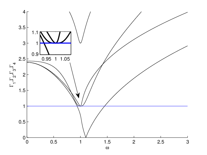
The above Puiseux series are consistent with the analysis by Theorem 5.2. In this case, for each $k$ , (i) the Puiseux series has multiple conjugacy classes; (ii) the Puiseux series involves many degenerate terms, and, finally, (iii) the structure of Puiseux series is variable w.r.t. different $k$ . It is evident that the FSC formalism significantly simplifies the analysis. $\Box$

In the sequel, we present an example reported in Li et al. 2019a to explicitly illustrate that the asymptotic behavior of a multiple characteristic root may lead to a stability reversal.

Example 5.5

Consider the quasipolynomial $\Delta(\lambda;\tau)=\lambda^{5}-\sum_{\ell=0}^{4}\alpha_{\ell}\lambda^{\ell}-(\sum_{\ell=0}^{4}\beta_{\ell}\lambda^{\ell})e^{-\tau\lambda}$ . where $\alpha_{0}=\frac{\pi}{2}-\frac{\pi^{2}}{8}-1$ , $\alpha_{1}=-2+\frac{\pi}{2}$ , $\alpha_{2}=-\frac{\pi^{2}}{4}+\pi-10$ , $\alpha_{3}=-3+\frac{\pi}{2}$ , $\alpha_{4}=-\frac{\pi^{2}}{8}+\frac{\pi}{2}-8$ , $\beta_{0}=-1$ , $\beta_{1}=-1$ , $\beta_{2}=-10$ , $\beta_{3}=-1$ , and $\beta_{4}=-8$ .
For this system, ${\rm NU}(\tau)=0$ for $\tau\in[0,1.2525)$ and ${\rm NU}(\tau)=2$ if $\tau\in(1.2525,\pi)$ . At $\tau=\pi$ , a critical imaginary root $\lambda=j$ with $n=2$ and $g=1$ appears, whose asymptotic behavior corresponds to the Puiseux series:

\delta\lambda=0.1468j(\delta\tau)^{\frac{1}{2}}+(-0.0033-0.1473j)(\delta\tau)+\ldots

It implies that when $\tau$ passes through $\pi$ , a stability reversal is caused by the asymptotic behavior of the double root $\lambda=j$ . The system possesses two and only two stability intervals of $\tau$ . More precisely, it is asymptotically stable iff $\tau\in[0,1.2525)\cup(\pi,4.0549)$ .

The asymptotic behavior issue and the stability can be easily addressed by using the frequency-sweeping approach (see Fig. 9). $\Box$

6 Multiple characteristic roots and multiple delays

Let us consider the following quasipolynomial:

\displaystyle\Delta(\lambda,\overrightarrow{\tau})

\displaystyle=\sum_{k=0}^{2}P_{k}(\lambda)e^{-\tau_{k}\lambda},\qquad\tau_{k}\geq 0,

(45)

where $\overrightarrow{\tau}:=\left(\tau_{1},\tau_{2}\right)$ , $\tau_{0}:=0$ , $\tau_{1},\tau_{2}\in\mathbb{R}_{+}$ and,

P_{0}(\lambda):=\lambda^{n}+\sum_{\ell=0}^{n-1}a_{0\ell}\lambda^{\ell},\,\,P_{k}(\lambda):=\sum_{\ell=0}^{n-1}a_{k\ell}\lambda^{\ell},\quad k=1,2.

This section focuses on computing the first approximation of the solution of quasipolynomials around multiple imaginary roots. To such an end, we will derive conditions allowing to express the solutions of $\Delta$ as a Puiseux series expansion, that is:

\lambda(\tau_{1},\tau_{2})=c(\tau_{2}^{1/d})\tau_{1}^{\beta}+o(\tau_{1}^{1/d}\tau_{2}^{1/d}),

where $\beta=\alpha/d$ and $\alpha\in\mathbb{N}$ .
Inspired by the approach adopted in Section 4, we will compute the associated Weierstrass polynomial of $\Delta$ . In this vein, following Mailybaev and Grigoryan 2001 for the case of a holomorphic function, $f(z,\overrightarrow{x})$ of complex variables with $\overrightarrow{x}=(x_{1},x_{2})$ and $z=0$ a $m$ -multiple root at $\left(x_{1},x_{2}\right)=\left(0,0\right)$ the computation is given as follows. The coefficients $w_{i}$ (20) are analytic, $w_{i}(0,0)=0$ and can expressed as convergent power series:

w_{i}(x_{1},x_{2})=\sum_{h_{1}+h_{2}=1}^{\infty}\frac{1}{h_{1}!h_{2}!}w_{i,\overrightarrow{h}}x_{1}^{h_{1}}x_{2}^{h_{2}},

where $\overrightarrow{h}=(h_{1},h_{2})$ . It is not difficult to see that the coefficients $w_{i,\overrightarrow{h}}$ can be computed as follows:

w_{i,\overrightarrow{h}}=\left.\frac{\partial^{h_{1}+h_{2}}w_{i}}{\partial x_{2}^{h_{1}}\partial x_{1}^{h_{2}}}\right|_{(0,0)}.

Since the analytic function locally satisfies $f=Wb$ , its partial derivatives satisfy the following recursive relations:

	$\displaystyle w_{i,\overrightarrow{h}}$	$\displaystyle=\sum_{r=0}^{i}\alpha_{ir}F_{r,\overrightarrow{h}},$		(46)
	$\displaystyle F_{r,\overrightarrow{h}}$	$\displaystyle=f_{r,\overrightarrow{h}}-\sum_{k=0}^{r}\sum_{\overrightarrow{h}^{\prime}+\overrightarrow{h}^{\prime\prime}=\overrightarrow{h}}\!\!\!\!\!c\!\left(r,k;\overrightarrow{h}^{\prime},\overrightarrow{h}^{\prime\prime}\right)w_{k,\overrightarrow{h}^{\prime}}b_{r-k,\overrightarrow{h}^{\prime\prime}},$

with $\overrightarrow{h}^{\prime}\neq\overrightarrow{0}$ , $\overrightarrow{h}^{\prime\prime}\neq\overrightarrow{0}$ and constant coefficients:

\alpha_{rr}:=\frac{m!}{r!f_{m,\overrightarrow{0}}},\quad\alpha_{ir}:=-\frac{m!}{f_{m,\overrightarrow{0}}}\sum_{k=r}^{i-1}\frac{f_{m+i-k,\overrightarrow{0}}\alpha_{kr}}{(m+i-k)!},

c\left(r,k;\overrightarrow{h}_{1},\overrightarrow{h}_{2}\right):=\frac{r!}{(r-k)!}\prod_{s=1}^{2}\frac{(h_{s}^{\prime}+h_{s}^{\prime\prime})!}{h_{s}^{\prime}!h_{s}^{\prime\prime}!},\\

and for $\overrightarrow{h}^{\prime}\neq 0$ , $k^{\prime}=k+m$ , $b_{k,\overrightarrow{h}}$ is given by

\!\!\frac{k!}{(m\!+\!k)!}\!\!\!\left[\!f_{k^{\prime},\overrightarrow{h}}-\!\!\sum_{r=0}^{m-1}\sum_{\overrightarrow{h}^{\prime}+\overrightarrow{h}^{\prime\prime}=\overrightarrow{h}}\!\!\!\!\!\!\!c\!\left(k^{\prime},r;\overrightarrow{h}^{\prime},\overrightarrow{h}^{\prime\prime}\!\right)\!\!w_{r,\overrightarrow{h}^{\prime}}b_{k^{\prime}-j,\overrightarrow{h}^{\prime\prime}}\!\right]\!\!.

In the sequel, we will adopt the following notations.

Definition 6.1

Let the natural numbers $n_{i}^{(r)}$ , for $i\in\llbracket 0,m-1\rrbracket$ and $r=1,2$ , denote the first nonzero partial derivative in $(z,x_{1},x_{2})$ of $f$ , such that:

f(0,0,0)\!=\!\frac{\partial^{i}f}{\partial z^{i}}\!=\cdots=\!\frac{\partial^{i+n_{i}^{(r)}-1}f}{\partial z^{i}\partial\tau_{r}^{n_{i}^{(r)}-1}}=0,\quad\frac{\partial^{i+n_{i}^{(r)}}f}{\partial z^{i}\partial\tau_{j}^{n_{i}^{(r)}}}\neq 0,

with derivatives evaluated at $(0,0,0)$ . For $n_{i}^{(r)}=\infty$ we have derivatives

\frac{\partial^{i}f}{\partial z^{i}}\!=\cdots=\frac{\partial^{i+n_{i}^{\prime}-1}f}{\partial z^{i}\partial\tau_{2}^{n_{i}^{\prime}-1}}=0,\quad\frac{\partial^{i+n_{i}^{\prime}}f}{\partial z^{i}\partial\tau_{2}^{n_{i}^{\prime}}}\neq 0,

evaluated at $(z,\overrightarrow{x})=(0,0,1)$ , with $n_{i}^{\prime}\in\mathbb{N}\cup\{0\}$ .

Leading terms of coefficients $w_{i}$ can be easy found up to the $n_{i}^{(r)}$ and $n_{i}^{\prime}$ derivatives. More precisely, as a first observation we give the following result:

Proposition 6.2

Suppose that the Weierstrass polynomial has first nonzero partial derivative, such that

n_{i}^{(r)}>n_{i+1}^{(r)},\quad 0\leq i<m\text{ and }r=1,2.

Then, the leading terms of $w_{i}(\overrightarrow{x})$ are given by

w_{i}(x_{1},x_{2})=\alpha_{i,i}f_{i,(n_{i}^{(1)},0)}x_{1}^{n_{i}^{(1)}}+\alpha_{i,i}f_{i,(0,n_{i}^{(2)})}x_{2}^{n_{i}^{(2)}}+\cdots.

If $n_{i}^{(r)}=\infty$ , we have

w_{i}(x_{1},x_{2})=\alpha_{i,i}f_{i,(n_{i}^{\prime},\eta)}x_{1}^{n_{i}^{\prime}}x_{2}^{\eta}+\cdots.

Remark 6.3

As in the single parameter case, there may be a situation in which

\left.f_{i,\overrightarrow{h}}\right|_{(0,0,0)}=0\quad\forall\;h_{1},h_{2}\in\mathbb{N}.

Since $w_{i}$ are analytic functions, this is equivalent to $w_{i}(\overrightarrow{x})\equiv 0$ for $i\leq i\leq\kappa-1$ . Thus, according to Theorem 4.1 $f$ has the following local structure:

z^{\kappa}\left[z^{m-\kappa}+w_{m-\kappa}(\overrightarrow{x})z^{m-\kappa-1}+\cdots+w_{\kappa}(\overrightarrow{x})\right]b(z,\overrightarrow{x}).

Thus, there are $\kappa$ -invariant solutions $z=0$ for all $\overrightarrow{x}$ . If such number $\kappa$ does not exist (i.e., if such situation does not occur), then $\kappa$ will be simply defined as $\kappa:=0$ . $\Box$

6.1 Newton diagram method: An extension

For a given $\pi_{k}\in\Pi$ , we consider the order of $w_{k}$ in $x_{1}$ , taking $x_{2}$ as an element of $\mathbb{C}\left[\left[x_{2}^{1/d}\right]\right]$ (for an appropriate $d\in\mathbb{N}$ ). For such a purpose, the following definition will be useful:

\rho_{k}:=\operatorname{ord}_{x_{1}}\left(w_{k}(x_{1},x_{2})\right)=\operatorname{ord}\left(w_{k}(x_{1},1)\right).

(47)

Then, the Newton polygon of $W_{p}(z,\overrightarrow{x})$ , with respect to $x_{1}$ , is defined by the lower boundary of the convex hull of the points $(k,\rho_{k})\in\Pi$ . Hence, in order to apply the the Newton diagram procedure, the solution $z$ will take the following structure

z(x_{1},x_{2})=\sum_{i}c_{i}(x_{2})x_{1}^{i/d},

where the coefficient $c_{i}(x_{2})$ , is in general, given by a single parameter Puiseux series in $x_{2}$ .
Therefore, with the aim to compute such a Puiseux series, let us suppose that we have determined the Newton diagram of the Weierstrass polynomial of $\Delta$ . Since we are dealing with a monic polynomial, the Newton polygon has a finite number of segments, each one with a corresponding set of points $\Pi^{(\ell)}$ and rational numbers $\beta_{\ell}\geq 0$ satisfying

\beta_{0}>\beta_{1}>\cdots>\beta_{r}.

In this regard, the segments are presented in two possible ways. The first one corresponds to a Newton polygon with a horizontal segment with $\beta_{i}=0$ , and the second one where $\beta_{j}>0$ (for $i\neq j$ ). In this vein, for $0\leq\ell<m$ , the Newton Diagram $\Pi$ is given as the set $\Pi=\Pi^{\prime}\cup\!\Pi^{\prime\prime}$ :

\left\{\!(0,\rho_{0}),\dots,\left(\ell,0\right)\!\right\}\cup\left\{\!\left(\ell,0\right),\dots,(k,\rho_{k}),\dots,\left(m,0\right)\!\right\}.

Assuming that at the first step of the process we found a horizontal segment with a slope $\beta_{r}=0$ , the following result allows characterizing the solution structure.

Proposition 6.4

Let $W_{p}(z,\overrightarrow{x})$ be a Weierstrass polynomial of a given quasipolynomial $\Delta$ . Suppose that at least one coefficient $w_{i}(\overrightarrow{\tau})$ possesses order $\rho_{i}=0$ . Then, the equation $\mathcal{P}_{i}(z;\tau_{1})=0$ of the corresponding $i$ -horizontal segment has solutions $c_{k}(\tau_{2}^{1/d})$ in the form of Puiseux series.

Remark 6.5

In the above result, $\mathcal{P}_{i}$ is built in the same fashion as in (26). $\Box$

Now, assuming that at the first step of the process we found a segment with a negative slope $\beta_{r}<0$ , the following result proposes an appropriate change of variable that will allow us to pursue the procedure.

Proposition 6.6

Let $W_{p}(z,\overrightarrow{\tau})$ be a Weierstrass polynomial of a given quasipolynomial $\Delta$ and assume that the first Newton diagram possesses a segment with negative slope. Then, there exist a change of variables $(\lambda,\tau_{1},\tau_{2})\mapsto(\xi,y_{1},y_{2})$ such that the polynomial $\mathcal{P}_{i}(z;y_{2})$ has Puiseux series solutions $c_{k}(y_{2}^{1/d})$ .

6.2 Puiseux series expansion

Since any critical solution $\left(\lambda^{\ast},\tau_{1}^{\ast},\tau_{2}^{\ast}\right)$ can always be translated to the origin by appropriate shifts $\lambda\mapsto\lambda-\lambda^{\ast}$ , $\tau_{1}\mapsto\tau_{1}-\tau_{1}^{\ast}$ , $\tau_{2}\mapsto\tau_{2}-\tau_{2}^{\ast}$ , hereinafter we will assume that $\left(\lambda^{\ast},\tau_{1}^{\ast},\tau_{2}^{\ast}\right)=(0,0,0)$ .

Proposition 6.7

Let $\lambda^{\ast}=j\omega^{\ast}$ be a $m$ -multiple root of $\Delta(\lambda,\overrightarrow{\tau})$ at $\overrightarrow{\tau}^{\ast}:=\left(\tau_{1}^{\ast},\tau_{2}^{\ast}\right)$ . Assume that $\kappa=0$ and $r$ , $\beta_{h}$ , $\left(i_{h},\ell_{h}\right)$ , $m_{h}$ and $\Pi^{(h)}$ , for $h\in\llbracket 0,r-1\rrbracket$ are given by the Algorithm 1. Then, at $\overrightarrow{\tau}=\overrightarrow{\tau}^{\ast}$ the $m$ -zeros of $\Delta(\lambda,\overrightarrow{\tau})$ can be expanded as

\lambda_{hq}(\overrightarrow{\tau})=j\omega^{\ast}+c_{hq}(\tau_{2})\left(\tau_{1}-\tau_{1}^{\ast}\right)^{\beta_{h}}\\ +o\left(\left|\tau_{1}-\tau_{1}^{\ast}\right|^{\beta_{h}}\left|\tau_{2}-\tau_{2}^{\ast}\right|^{\beta_{h}^{\prime}}\right),

for $h\in\llbracket 0,r-1\rrbracket$ , $q\in\llbracket 0,m_{h}\rrbracket$ and $m=m_{0}+\cdots+m_{r-1}$ . For $\beta_{h}>0$ , $c_{hq}(\tau_{2})$ are roots of the polynomial:

\mathcal{P}_{h}(z;\tau_{2})\!=\!\!\!\sum_{k=i_{h-1}}^{i_{h}}\!\!\!w_{k,(n_{k}^{(1)},n_{k}^{\prime})}\tau_{2}^{n_{k}^{\prime}}z^{k-i_{h-1}}\!,\quad\left(k,n_{k}^{(1)}\right)\!\in\!\Pi^{(h)},

when $\beta_{r-1}=0$ , the coefficients are given by the solution of

\mathcal{P}_{h}(z;\tau_{2})\!=\!\!\!\sum_{k=i_{h-1}}^{i_{h}}\!\!\!w_{k,(0,n_{k}^{(2)})}\tau_{2}^{n_{k}^{(2)}}\!z^{k-i_{q-1}}\!,\quad\left(k,0\right)\!\in\!\Pi^{(r-1)},

where $n_{k}^{(1)}$ , $n_{k}^{(2)}$ , $n_{k}^{\prime}$ are given by the first nonzero partial derivatives of Definition 6.1; the constant terms $w_{k,(n,\eta)}\in\mathbb{C}$ are computed using (46).

To illustrate the previous results, consider the following:

Example 6.8

Consider the quasipolynomial $\Delta(\lambda;\tau_{1},\tau_{2})\allowbreak:=P_{0}(\lambda)+P_{1}(\lambda)e^{-\tau_{1}\lambda}+P_{2}(\lambda)e^{-\tau_{2}\lambda}$ where


$\displaystyle P_{0}(\lambda)$	$\displaystyle:=$	$\displaystyle\lambda^{5}\!+\!\lambda^{4}\!+\!\frac{4+\pi}{2}\lambda^{3}\!+\!2\lambda^{2}\!+\!\frac{2+\pi}{2}\lambda\!+\!2,$	(48a)
$\displaystyle P_{1}(\lambda)$	$\displaystyle:=$	$\displaystyle 1,\quad P_{2}(\lambda):=2\lambda^{4}\!+\!4\lambda^{2}+2.$	(48b)

For $\overrightarrow{\tau}^{\ast}=(\pi,1)$ , $\Delta$ has a double root at $\lambda=j$ . The shifting from $(j,\pi,1)$ to the origin leads to $\widetilde{\Delta}$ . Next, by computing the first nonzero partial derivatives of the quasipolynomial at $(0,0,0)$ , one gets:

\Delta_{0,(1,0)}=j\;\,\,\,\,\,\,\,\,\,\,\,\,\,\,\Rightarrow n_{0}^{(1)}=1,\quad\Delta_{0,(0,n)}=0\Rightarrow n_{0}^{(2)}=\infty,

\Delta_{1,(1,0)}=1-j\pi\Rightarrow n_{1}^{(1)}=1,\quad\Delta_{1,(0,n)}=0\Rightarrow n_{1}^{(2)}=\infty.

Hence, by Proposition 6.2, we have that $\rho_{h}=n_{h}^{(1)}$ for $h=1,2$ . The Newton diagram is given by $\Pi=\{(0,1),(1,1),(2,0)\}$ . Table 2 summarizes the results deriving from Algorithm 1.

Table 2: Results summary for

\Delta

given by (48).

Initial Data	Algorithm Output	$\mathcal{Z}:=\left\{z\in\mathbb{C}:\;\mathcal{P}_{h}(z)=0\right\}$
$m=2$ , $\kappa=0$ . $\rho_{0}=1$	$r=1$ , $m_{0}=2$ , $\beta_{0}=1/2$	$\mathcal{P}_{0}(z):=z^{2}+w_{0,(1,0)}$
$\Pi=\left\{(0,1),(1,1),(2,0)\right\}$	$\Pi^{{}^{(0)}}=\left\{(0,1),(2,0)\right\}$	$\left\{c_{0,q}=\pm\sqrt{w_{0,(1,0)}}\right\}$

Since $w_{1}$ is not over the Newton polygon, following Proposition 6.2, we compute the leading term of $w_{i}(\overrightarrow{\tau})$ as:

w_{0}(\overrightarrow{\tau})=\frac{-2j}{(8+\pi^{2})+j(8-3\pi)+16e^{-j}}\tau_{1}+\cdots.

From the algorithm output, we get a segment with slope $\beta_{0}=1/2$ . According to Proposition 6.7, we need to solve:

\mathcal{P}_{0}(z)=z^{2}-\frac{2j}{(8+\pi^{2})+j(8-3\pi)+16e^{-j}}=0,

and, for $q\in\{0,1\}$ , the solutions are given by

\lambda_{0,q}(\overrightarrow{\tau})\!=\!j+\frac{(-1)^{q}\sqrt{2}j^{3/2}}{\sqrt{(8\!+\!\pi^{2})\!+\!j(8\!-\!3\pi)\!+\!16e^{-j}}}(\tau_{1}\!-\!\pi)^{1/2}+\cdots.

Remark 6.9

It is worth mentioning that the frequency-sweeping approach can be also extended to handle multiple characteristic roots on imaginary axis for delay systems including incommensurate delays, see, e.g. Li et al. 2019b for an iterative frequency-sweeping method. $\Box$

7 Hypergeometric functions and multiplicity-induced-dominancy

We consider in this section the DDE given by:

y^{(n)}(t)+\sum_{k=0}^{n-1}a_{k}y^{(k)}(t)+\sum_{k=0}^{m}\alpha_{k}y^{(k)}(t-\tau)=0,

(49)

where $y$ is real-valued, $n$ is a positive integer, $m\in\llbracket 0,n\rrbracket$ , $\tau>0$ is the delay, and $a_{0},\dotsc,a_{n-1},\alpha_{0},\dotsc,\alpha_{m}$ are real coefficients. Its characteristic function is

\Delta(\lambda;\overrightarrow{a},\overrightarrow{\alpha})=\lambda^{n}+\sum_{k=0}^{n-1}a_{k}\lambda^{k}+e^{-\lambda\tau}\sum_{k=0}^{m}\alpha_{k}\lambda^{k}.

(50)

The problem of characterizing regions in the space of parameters of (49) ensuring exponential stability is a highly non-trivial problem of ongoing interest, and, thanks to classical results, such a problem is equivalent to characterizing regions in the space of the coefficients of (50) ensuring that all its roots $\lambda$ satisfy $\Re(\lambda)\leq-\gamma$ for some $\gamma>0$ (see, e.g., Michiels and Niculescu 2014). This question is naturally related to control-theoretical problems, since (49) can be seen as the closed-loop system obtained by applying a linear (possibly delayed) feedback law to a controlled delay-differential equation, and in this case, by suitably choosing the coefficients of the feedback law, one may choose (some of) the coefficients of (49).
Since (50) admits infinitely many roots but has only $m+n+1$ parameters, one cannot expect to be able to choose arbitrarily the location in $\mathbb{C}$ of all roots of $\Delta$ . Some works are interested in methods to choose the location of finitely many roots of $\Delta$ , trying to guarantee that the other roots have negative real part and are separated from the imaginary axis, a technique known as partial pole placement. Trial-and-error methods, such as those in Ram et al. 2011, have been proposed in the literature, but techniques guaranteeing that the non-assigned roots have negative real part are more difficult to obtain. The numerical paradigm known as continuous pole placement, introduced in Michiels et al. 2002, exploits continuity of roots of $\Delta$ with respect to the coefficients of the system in order to move roots with positive real part to the left half-plane while ensuring that no stable roots becomes unstable.

In the sequel, we present a recent technique for partial pole placement, based on the property known as multiplicity-induced-dominancy, or MID for short (see, e.g., Boussaada et al. 2020). The MID property states that, if a real root of (50) attains its maximal multiplicity (which is equal to $m+n+1$ , cf. Remark 2.5), then this root necessarily is the rightmost root in the complex plane. Hence, a technique for partial pole placement based on the MID property consists in choosing the coefficients of the system in order to ensure the existence of a negative real root of maximal multiplicity. More precisely, we have the following:

Theorem 7.1

Consider the quasipolynomial $\Delta$ given by (50) and let $\lambda_{0}\in\mathbb{R}$ . The number $\lambda_{0}$ is a root of maximal multiplicity $m+n+1$ of $\Delta$ if and only if

	$\displaystyle a_{k}$	$\displaystyle=\left(-1\right)^{n-k}n!\,\sum_{i=k}^{n}{\frac{\binom{i}{k}\binom{m+n-i}{m}\lambda_{0}^{i-k}}{i!\,{\tau}^{n-i}}},\quad k\leq n-1,$		(51)
	$\displaystyle\alpha_{k}$	$\displaystyle=\left(-1\right)^{n-1}{{e}^{\lambda_{{0}}\tau}}\sum_{i=k}^{m}{\frac{\left(-1\right)^{i-k}\left(m+n-i\right)!\,\lambda_{0}^{i-k}}{k!\,\left(i-k\right)!\,\left(m-i\right)!\,{\tau}^{n-i}}},k\leq m.$		(51)

If $m<n$ and (51) is satisfied, then $\Re(\lambda)<\lambda_{0}$ for every root $\lambda\neq\lambda_{0}$ of $\Delta$ . If $m=n$ and (51) is satisfied, then $\Re(\lambda)=\lambda_{0}$ for every root $\lambda$ of $\Delta$ . In particular, the trivial solution of (49) is exponentially stable if and only if $a_{n-1}>-\frac{n(m+1)}{\tau}$ .

Theorem 7.1 was proved in the case $m=n-1$ in Mazanti et al. 2021 and extended to any $m\in\llbracket 0,n\rrbracket$ (including thus the neutral case $m=n$ ) in the recent paper Boussaada et al. 2021a. Let us briefly present the main ideas of its proof. Up to a change of variables corresponding to a translation and a scaling, it suffices to prove the theorem in the case $\tau=1$ and the desired root of maximal multiplicity is at the origin, i.e., $\lambda_{0}=0$ . In this case, $\lambda_{0}=0$ is a root of maximal multiplicity $m+n+1$ if and only if $\Delta(0)=\dotsb=\Delta^{(m+n)}(0)=0$ , which gives a linear system in the $m+n+1$ coefficients $a_{0},\dotsc,a_{n-1},\alpha_{0},\dotsc,\alpha_{m}$ admitting (51) as its unique solution.

To prove the properties on the dominance of $\lambda_{0}$ , the main ingredient is that, under (51) and with $\tau=1$ and $\lambda_{0}=0$ , $\Delta$ can be factorized as

\Delta(\lambda;\overrightarrow{a},\overrightarrow{\alpha})=\frac{n!\lambda^{m+n+1}}{(m+n+1)!}\Phi(m+1,m+n+2,-\lambda),

where $\Phi$ is Kummer confluent hypergeometric function, which admits the integral representation

\Phi(a,b,z)=\frac{\Gamma(b)}{\Gamma(a)\Gamma(b-a)}\int_{0}^{1}t^{a-1}(1-t)^{b-a-1}e^{zt}dt

for every $a,b,z\in\mathbb{C}$ with $\Re(b)>\Re(a)>0$ , where $\Gamma$ denotes the Gamma function. In particular, proving the last part of Theorem 7.1 amounts to showing that all roots of $\Phi(m+1,m+n+2,\cdot)$ have positive real part if $m<n$ and real part zero if $m=n$ . As detailed in Boussaada et al. 2021b, these facts can be established by applying the technique developed in Hille 1922 to a family of special functions related to Kummer functions, known as Whittaker functions, and exploring the fact that Whittaker functions satisfy a second-order ordinary differential equation.

7.1 Inverted pendulum: Delay, PD control & MID

The MID property may hold even when the multiplicity of a given quasipolynomial’s root does not reach its maximal value. Hereafter, we illustrate such a claim on the standard comprehensive problem of the stabilization of the inverted pendulum. The equation of motion of an inverted pendulum controlled by a delayed PD-controller writes as:

		$\displaystyle\ddot{\varphi}(t)+a_{0}\varphi(t)=u(t)\,,$		(52)
		$\displaystyle u(t)=-b_{0}\varphi(t-\tau)-b_{1}\dot{\varphi}(t-\tau)\,,$		(52)

with $\tau>0$ and $a_{0}<0$ . The characteristic function corresponding to (52) is:

\Delta(\lambda;b_{0},b_{1},\tau)=P_{0}(\lambda)+P_{1}(\lambda)\,e^{-\lambda\tau},

(53)

with $P_{0}(\lambda)=\lambda^{2}+a_{0}$ and $P_{1}(\lambda;b_{0},b_{1})=b_{0}+b_{1}\lambda$ . The critical delay of system (52) is given by:

\tau_{\mathrm{crit}}=\sqrt{-\tfrac{2}{a_{0}}}\,,

(54)

that is, the closed-loop system (52) is asymptotically stable if and only if $\tau<\tau_{\mathrm{crit}}$ . The critical delay (54) can be obtained by studying the multiple roots of $\Delta(\cdot;b_{0},b_{1},\tau)$ . Indeed, assume that $\Delta$ has a real root $\lambda_{0}$ with algebraic multiplicity at least $\mathrm{deg}P(\lambda)+1=3$ . Then $\Delta(\lambda_{0};b_{0},b_{1},\tau)=\Delta^{\prime}(\lambda_{0};b_{0},b_{1},\tau)=\Delta^{\prime\prime}(\lambda_{0};b_{0},b_{1},\tau)=0$ give

\left\{\begin{aligned} \lambda_{0}^{2}+a_{0}+e^{-\lambda_{0}\tau}(b_{0}+b_{1}\lambda_{0})&=0\,,\\ 2\lambda_{0}+e^{-\lambda_{0}\tau}(-\tau(b_{0}+b_{1}\lambda_{0})+b_{1})&=0\,,\\ 2+e^{-\lambda_{0}\tau}(\tau^{2}(b_{0}+b_{1}\lambda_{0})-2\tau b_{1})&=0\,.\end{aligned}\right.

(55)

From (55) we obtain

\left\{\begin{aligned} b_{0}&=e^{\lambda_{0}\tau}\left(\tau\lambda_{0}^{3}+\lambda_{0}^{2}+a_{0}\tau\lambda_{0}-a_{0}\right)\,,\\ b_{1}&=-e^{\lambda_{0}\tau}\left(\tau\lambda_{0}^{2}+2\lambda_{0}+a_{0}\tau\right)\,,\\ \lambda_{0}&=\frac{-2\pm\sqrt{2-a_{0}\tau^{2}}}{\tau}\eqqcolon\lambda_{\pm}.\end{aligned}\right.

(56)

It can be shown that the triple root $\lambda_{+}$ is negative and dominant for every $0<\tau<\tau_{\mathrm{crit}}$ , and therefore system (52) is asymptotically stable, see, e.g., Boussaada et al. 2017; Boussaada et al. 2020. In particular, at the upper bound $\tau=\tau_{\mathrm{crit}}$ the triple root is $\lambda_{+}=0$ and it is the dominant (rightmost) root of (53) with control “gains” $b_{0}=-a_{0}$ and $b_{1}=-a_{0}\tau_{\mathrm{crit}}$ . Alternatively, for a given $\lambda_{+}=\gamma<0$ , (55) can be solved for $b_{0}$ , $b_{1}$ and $\tau$ . The smallest positive solution for $\tau$ is the critical delay $\tau_{\mathrm{crit}}(\gamma)$ associated with $\gamma$ -stability.

Remark 7.2

The dominancy of $\lambda_{+}$ has been shown by using the argument principle, see, for instance (Boussaada et al. 2020). A constructive proof of the dominancy of $\lambda_{+}$ may be also shown using the corresponding quasipolynomial factorization introduced in Bedouhene et al. 2020 and recently extended in Balogh et al. 2022 to arbitrary order systems such that in open-loop they admit only real-rooted modes. $\Box$

7.2 A control oriented MID property

In this section we consider delayed feedback systems whose characteristic function is a quasipolynomial of the form

\Delta(\lambda;\overrightarrow{b},\tau)=P_{0}(\lambda)+P_{1}(\lambda,\overrightarrow{b})\,e^{-\lambda\tau},

(57)

where $\tau\in\mathbb{R}_{+}$ , $\mathrm{deg}(P_{0})=n$ , $\mathrm{deg}(P_{1})=n-1$ . Assume that the coefficients of $P_{0}$ are known and that $\overrightarrow{b}\in\mathbb{R}^{n}$ denotes the parameter vector including the coefficients of $P_{1}$ . Assume further that the coefficients $b_{i}$ are independently adjustable) control parameters:

	$\displaystyle P_{0}(\lambda)$	$\displaystyle=a_{n}\lambda^{n}+a_{n-1}\lambda^{n-1}+\dotsb+a_{1}\lambda+a_{0}\,,$		(58)
	$\displaystyle P_{1}(\lambda;\overrightarrow{b})$	$\displaystyle=b_{n-1}\lambda^{n-1}+b_{n-2}\lambda^{n-2}+\dotsb+b_{1}\lambda+b_{0}\,.$		(58)

The problem to be considered is to find the values of $\tau$ such that (57) is $\gamma$ -stabilizable. To give a sufficient condition for $\gamma$ -stabilizability²⁶²⁶ 26 In other words, the spectral abscissa $\alpha_{s}$ of the closed-loop system should verify the condition $\alpha_{s}\leq\gamma$ for the corresponding set of parameters. we utilize the MID-property: the control parameters $b_{i}$ are tuned such that the characteristic function $\Delta(\lambda)$ has a real root $\lambda_{0}$ with multiplicity $n+1$ . The result from Balogh et al. 2022 emphasizes the way to factorize a quasipolynomial admitting a multiple root.

Proposition 7.3

If the quasipolynomial (57)-(58) admits a real root $\lambda_{0}$ with multiplicity at least $n$ then $\Delta(\lambda;\overrightarrow{b},\tau)=$

(\lambda-\lambda_{0})^{n}\left(a_{n}+\int_{0}^{1}e^{-(\lambda-\lambda_{0})\tau t}\frac{\tau R_{n-1}(\lambda_{0};\tau t)}{(n-1)!}\mathrm{d}t\right)\,,

(59)

where the family of polynomials $R_{k}(\lambda;\tau)$ is defined as

R_{k}(\lambda;\tau)=\sum_{i=0}^{k}\binom{k}{i}P_{0}^{(i)}(\lambda)\tau^{k-i},\,k\in\mathbb{N}^{*}\,.

(60)

Some sufficient conditions for the dominancy are given by:

Proposition 7.4

Let $\lambda_{0}$ be a real root of the quasipolynomial (57) with multiplicity at least $n+1$ . If $R_{n-1}(\lambda_{0};\tau t)\leq 0$ , $\forall t$ , $0<t\leq 1$ then $\lambda_{0}$ is the dominant root of (57).

7.3 Imaginary roots, MID & applications

We consider in this subsection a retarded delay-differential equation of second order under the form $\ddot{y}(t)+a_{1}\dot{y}(t)+a_{0}y(t)+\alpha_{1}\dot{y}(t-\tau)+\alpha_{0}y(t-\tau)=0$ , where $a_{1},a_{0},\alpha_{1},\alpha_{0}$ are real parameters to be tuned. Its characteristic function is the quasipolynomial $\Delta$ defined by

\Delta(\lambda)=\lambda^{2}+a_{1}\lambda+a_{0}+(\alpha_{1}\lambda+\alpha_{0})\,e^{-\lambda\tau}.

(61)

All previous results on multiplicity-induced-dominancy concern only real roots with high multiplicity, and a natural question is whether one may choose as dominant roots a pair of complex-conjugate nonreal multiple roots. The answer, at least for (61), is affirmative, as stated in the next result.

Theorem 7.5

Let $\lambda_{0}\in\mathbb{C}$ , denote $\sigma_{0}=\Re(\lambda_{0})$ and $\theta_{0}=\Im(\lambda_{0})$ , and assume that $\theta_{0}\neq 0$ . Then $\lambda_{0}$ and its conjugate $\overline{\lambda}_{0}$ are roots of multiplicity $2$ of $\Delta$ from (61) if and only if


$\displaystyle a_{1}$	$\displaystyle\textstyle=-2\sigma_{0}-\theta_{0}\frac{2\tau\theta_{0}-\sin(2\tau\theta_{0})}{\tau^{2}\theta_{0}^{2}-\sin^{2}(\tau\theta_{0})},$	(62a)
$\displaystyle a_{0}$	$\displaystyle\textstyle=\sigma_{0}^{2}+\frac{\sigma_{0}\theta_{0}(2\tau\theta_{0}-\sin(2\tau\theta_{0}))+\tau^{2}\theta_{0}^{4}+\theta_{0}^{2}\sin^{2}(\tau\theta_{0})}{\tau^{2}\theta_{0}^{2}-\sin^{2}(\tau\theta_{0})},$	(62b)
$\displaystyle\alpha_{1}$	$\displaystyle\textstyle=2\theta_{0}e^{\sigma_{0}\tau}\frac{\tau\theta_{0}\cos(\tau\theta_{0})-\sin(\tau\theta_{0})}{\tau^{2}\theta_{0}^{2}-\sin^{2}(\tau\theta_{0})},$	(62c)
$\displaystyle\alpha_{0}$	$\displaystyle\textstyle=2\theta_{0}e^{\sigma_{0}\tau}\frac{(\sigma_{0}-\tau\theta_{0}^{2})\sin(\tau\theta_{0})-\tau\sigma_{0}\theta_{0}\cos(\tau\theta_{0})}{\tau^{2}\theta_{0}^{2}-\sin^{2}(\tau\theta_{0})}$	(62d)

Moreover, if (62) is satisfied, then all roots $\lambda$ of $\Delta$ which are different from $\lambda_{0}$ and from $\overline{\lambda}_{0}$ satisfy $\Re(\lambda)<\Re(\lambda_{0})$ .

As $\theta_{0}\to 0$ , the expressions in (62) converge to those for the existence of a real root of multiplicity $4$ at $\lambda=\sigma_{0}$ , as stated in Theorem 7.1, for which it is known that $\sigma_{0}$ is dominant. The proof of Theorem 7.5, presented in Mazanti et al. 2020, uses this fact and the continuity of roots as functions of $\theta_{0}$ in order to show that dominance of the roots $\lambda_{0}$ and $\overline{\lambda}_{0}$ is preserved as $\theta_{0}$ increases from $0$ to any positive value, taking appropriate care of possible roots coming from $\infty$ .

Based on Mazanti et al. 2020, we illustrate the application of Theorem 7.5 to active vibration suppression (AVS), in which we desire to suppress vibrations from an excitation force of a known frequency $\omega$ (see Fig. 10). The system main body is a vibrating platform $P$ excited by a periodic external force $f(t)=F\cos(\omega t)$ , and the absorber $A$ is actuated with the active feedback $u(t)$ to compensate the vibrations. The absorber dynamics is then $\ddot{x}_{a}(t)+2\zeta\Omega\dot{x}_{a}(t)+\Omega^{2}x_{a}(t)=\frac{1}{m_{a}}u(t)$ .

Remark 7.6

The delayed resonator scheme by Olgac and Holm-Hansen 1994 consists in guaranteeing vibration suppression by ensuring the overall system to have zeros at $\pm j\omega$ , and we adapt that scheme here by placing zeros of multiplicity two at $\pm j\omega$ using Theorem 7.5. For a different adaptation, we refer to Kuře et al. 2018. $\Box$

Choosing the delay as $\tau_{k}=\frac{k\pi}{\omega}$ for some $k\in\mathbb{N}^{\ast}$ , Theorem 7.5 ensures that $\pm j\omega$ is a double root of $\Delta$ if and only if

\Delta_{\omega}(\lambda)=\lambda^{2}+\frac{2}{\tau_{k}}\left((-1)^{k}e^{-\lambda\tau_{k}}-1\right)s+\omega^{2}.

(63)

Introducing the active feedback $u(t)=m_{a}(\Omega^{2}-\omega^{2})x_{a}(t)+2m_{a}\bigl(\zeta\Omega+\frac{1}{\tau_{k}}\bigr)\dot{x}_{a}(t)-2m_{a}\frac{(-1)^{k}}{\tau_{k}}\dot{x}_{a}(t-\tau_{k})$ , the characteristic function of the active absorber is given by (63), with a double root at $\pm j\omega$ . As shown, e.g., in Kuře et al. 2018, the transfer function $f\rightarrow x_{p}$ is in the form $G(\lambda)=\frac{\Delta_{\omega}(\lambda)}{M(\lambda)}$ . Therefore, as required, the double roots at $\pm j\omega$ become double zeros of $G_{x_{a}f}$ , implying that no vibrations are transferred from $f$ to $x_{p}$ and the platform is fully silenced.

8 Concluding remarks

This paper presents several approaches and methods for handling multiple characteristic roots in time-delay systems represented by linear DDEs. More precisely, perturbation theory techniques, frequency-sweeping based approach and multiplicity-induced-dominancy method are explicitly discussed. For a better understanding of the concepts, notions as well as of the proposed methods, several illustrative examples complete the presentation.

Acknowledgements

The authors wish thank Jie Chen, Keqin Gu, Tamas Insperger, Wim Michiels, Rifat Sipahi and Tomas Vyhlidal for useful discussions concerning the topics of the paper. C.F. Méndez-Barríos gratefully acknowledges the financial support of CentraleSupélec (France) and CONACyT (Mexico) which supported several short stays of the author in France (2018-2021). X.-G. Li’s work was supported in part by Fundamental Research Funds for the Central Universities (No. N2104007).

References

Ahlfors (1979) Ahlfors, L.V. (1979). Complex Analysis. International Series in Pure and Applied Mathematics. McGraw-Hill.
Asl and Galip Ulsoy (2003) Asl, A.M. and Galip Ulsoy, A. (2003). Analysis of a system of linear delay differential equations. ASME J. Dyn. Syst. Meas. Contr., 125(2), 215–223.
Atay (1999) Atay, F.M. (1999). Balancing the inverted pendulum using position feedback. Appl. Math. Lett., 12(5), 51–56.
Balogh et al. (2022) Balogh, T., Boussaada, I., Insperger, T., and Niculescu, S.I. (2022). Condition for stabilizability of time-delay systems with real-rooted plant. Int. J. Robust Nonlin. Contr., (to appear).
Barker (1979) Barker, L.K. (1979). Mikhailov stability criterion for time-delayed systems. Technical Memorandum TM-78803, NASA, Washington D. C., USA.
Bedouhene et al. (2020) Bedouhene, F., Boussaada, I., and Niculescu, S.I. (2020). Real spectral values coexistence and their effect on the stability of time-delay systems: Vandermonde matrices and exponential decay. C. R. Math. Acad. Sci. Paris, 358(9-10), 1011–1032.
Bellman and Cooke (1963) Bellman, R. and Cooke, K. (1963). Differential-difference equations. Academic Press, New York.
Boussaada et al. (2015) Boussaada, I., Morărescu, I.C., and Niculescu, S.I. (2015). Inverted pendulum stabilization: Characterization of codimension-three triple zero bifurcation via multiple delayed proportional gains. Syst. Contr. Lett., 82, 1–9.
Boussaada and Niculescu (2016a) Boussaada, I. and Niculescu, S.I. (2016a). Characterizing the codimension of zero singularities for time-delay systems. Acta Applicandae Math., 145(1), 47–88.
Boussaada and Niculescu (2016b) Boussaada, I. and Niculescu, S.I. (2016b). Tracking the algebraic multiplicity of crossing imaginary roots for generic quasipolynomials: A Vandermonde-based approach. IEEE Trans. Automat. Contr., 61, 1601–1606.
Boussaada et al. (2021a) Boussaada, I., Mazanti, G., and Niculescu, S.I. (2021a). The generic multiplicity-induced-dominancy property from retarded to neutral delay-differential equations: When delay-systems characteristics meet the zeros of kummer functions. ArXiv:2107.11363.
Boussaada et al. (2021b) Boussaada, I., Mazanti, G., and Niculescu, S.I. (2021b). Some remarks on the location of non-asymptotic zeros of whittaker and kummer hypergeometric functions. ArXiv:2106.03378.
Boussaada et al. (2020) Boussaada, I., Niculescu, S.I., El-Ati, A., Pérez-Ramos, R., and Trabelsi, K. (2020). Multiplicity-induced-dominancy in parametric second-order delay differential equations: analysis and application in control design. ESAIM Control Optim. Calc. Var., 26, Paper No. 57, 34.
Boussaada et al. (2017) Boussaada, I., Tliba, S., Niculescu, S.I., Unal, H.U., and Vyhlidal, T. (2017). Further remarks on the effect of multiple spectral values on the dynamics of time-delay systems. application to the control of a mechanical system. Linear Algebra Appl.
Cai et al. (2014) Cai, T.Y., Zhang, H., Wang, B., and Yang, F. (2014). The asymptotic analysis of multiple imaginary characteristic roots for lti delayed systems based on Puiseux–Newton diagram. Int. J. Syst. Sci., 45(5), 1145–1155.
Chen and Tsay (1976) Chen, C.F. and Tsay, Y.T. (1976). A general frequency stability criterion for multi-input-output, lumped and distributed-parameter systems. Int. J. Contr., 23(3), 341–359.
Chen (1995) Chen, J. (1995). On computing the maximal delay intervals for stability of linear delay systems. IEEE Trans. Automat. Contr., 40(6), 1087–1093.
Chen et al. (2010a) Chen, J., Fu, P., Niculescu, S.I., and Guan, Z. (2010a). An eigenvalue perturbation approach to stability analysis, Part i : Eigenvalue series of matrix operator. SIAM Journal on Optimization and Control, 48, 5564–5582.
Chen et al. (2010b) Chen, J., Fu, P., Niculescu, S.I., and Guan, Z. (2010b). An eigenvalue perturbation approach to stability analysis, Part ii : When will zeros cross imaginary axis? SIAM Journal on Optimization and Control, 48, 5583–5605.
Chen et al. (1995) Chen, J., Gu, G., and Nett, C.A. (1995). A new method for computing delay margins for stability of linear delay systems. Syst. Contr. Lett., 26, 107–117.
Chen and Latchman (1995) Chen, J. and Latchman, H.A. (1995). Frequency sweeping tests for stability independent of delay. IEEE Trans. Automat. Contr., 40(9), 1640–1645.
Chen et al. (2017) Chen, J., Fu, P., Méndez-Barrios, C.F., Niculescu, S.I., and Zhang, H. (2017). Stability analysis of polynomially dependent systems by eigenvalue perturbation. IEEE Transactions on Automatic Control, 62(11), 5915–5922.
Chi et al. (2018) Chi, J., Gu, K., Niculescu, S.I., and Boussaada, I. (2018). Stability analysis of systems with delay-dependent coefficients: An overview. IEEE Access, 6, 27392–27407.
Chosky (1960) Chosky, N.H. (1960). Time lag systems — A bibliography. IRE Trans. Automat. Contr., AC-5(1), 66–70.
Cooke and Grossman (1982) Cooke, K.L. and Grossman, Z. (1982). Discrete delay, distributed delay and stability switches. J. Math. Anal. Appl., 86, 592–627.
Cooke and van den Driessche (1986) Cooke, K.L. and van den Driessche, P. (1986). On zeroes of some transcendental equations. Funkcial. Ekvac., 29(1), 77–90.
Corless et al. (1996) Corless, R., Gonnet, G.H., Hare, D.E.G., Jeffrey, D.J., and Knuth, D.E. (1996). On the Lambert W function. Adv. Comput. Math., 5(3), 329–359.
Datko (1978) Datko, R. (1978). A procedure for determination of the exponential stability of certain differential-difference equations. Quarterly of Applied Mathematics, 36, 279–292.
Els’golts’ and Norkin (1973) Els’golts’, L.E. and Norkin, S.B. (1973). Introduction to the theory and application of the theory of differential equations with deviating argument. Academic Press: New York, New York.
Evans (1950) Evans, W.E. (1950). Control system synthesis by root locus method. AIEE Transactions, 69, 66–69.
Fridman (2014) Fridman, E. (2014). Introduction to time-delay systems: Analysis and control. Birkhauser: Boston.
Gu et al. (2003) Gu, K., Kharitonov, V.L., and Chen, J. (2003). Stability of Time-Delay Systems. Birkhauser: Boston.
Halanay (1966) Halanay, A. (1966). Differential Equations: Stability, Oscillations, Time Lags. Academic Press: New York.
Hale (2006) Hale, J.K. (2006). History of delay equations, 1–28. Springer Verlag, New York.
Hale et al. (1985) Hale, J.K., Infante, E.F., and Tsen, F.S.P. (1985). Stability in linear delay equations. Journal of Mathematical Analysis and Applications, 105(2), 533–555.
Hale and Verduyn Lunel (1993) Hale, J.K. and Verduyn Lunel, S.M. (1993). Introduction to functional differential equations, volume 99 of Applied Mathematics Sciences. Springer Verlag, New York.
Hassard (1997) Hassard, B. (1997). Counting roots of the characteristic equation for linear delay-differential systems. Journal of Differential Equations, 136(2), 222–235.
Hayes (1950) Hayes, N.D. (1950). Roots of the transcendental equation associated with a certain difference-differential equation. J. London Math. Soc., s1-25(3), 226–232.
Hille (1922) Hille, E. (1922). Oscillation theorems in the complex domain. Trans. Amer. Math. Soc., 23(4), 350–385.
Jarlebring and Michiels (2010) Jarlebring, E. and Michiels, W. (2010). Invariance properties in the root sensitivity of time-delay systems with double imaginary roots. Automatica, 46(6), 1112–1115.
Kamen (1982) Kamen, E.W. (1982). Linear systems with commensurate time delays: stability and stabilization independent of delay. IEEE Trans. Automat. Contr., AC-27(2), 367–375.
Kappel (2006) Kappel, F. (2006). Linear autonomous functional differential equations, 41–139. Springer Verlag, New York.
Kashiwagi (1965) Kashiwagi, Y. (1965). Stability of linear systems with time-delay. Ph.D. thesis, Stanford Univ.
Kharitonov et al. (2005) Kharitonov, V., Niculescu, S.I., Moreno, J., and Michiels, W. (2005). Static output feedback stabilization: necessary conditions for multiple delay controllers. IEEE Trans. Automat. Cont., 50(1), 82–86.
Krall (1965) Krall, A.M. (1965). Stability criteria for feedback systems with a time lag. SIAM J Contr, Ser. A, 2, 160–170.
Krall (1968) Krall, A.M. (1968). Stability techniques for continuous linear systems. Gordon and Breach: New York.
Krall (1970) Krall, A.M. (1970). The root locus method: A survey. SIAM Review, 12(1), 64–72.
Kuře et al. (2018) Kuře, M., Vyhlídal, T., Michiels, W., and Boussaada, I. (2018). Spectral design of robust delayed resonator by double-root assignment. IFAC-PapersOnLine, 51(14), 72–77.
Lee and Hsu (1969) Lee, M.S. and Hsu, C.S. (1969). On the $\tau$ -decomposition method of stability analysis for retarded dynamical systems. SIAM Journal of Control, 7, 242–259.
Li et al. (2019a) Li, X., Liu, J.C., Li, X.G., Niculescu, S.I., and Çela, A. (2019a). Reversals in stability of linear time-delay systems: A finer characterization. Automatica, 108(4), 108479.
Li et al. (2017) Li, X.G., Niculescu, S.I., A. Çela, A., Zhang, L., and Li, X. (2017). A frequency-sweeping framework for stability analysis of time-delay systems. IEEE Transactions on Automatic Control, 62(8), 3701–3716.
Li et al. (2019b) Li, X.G., Niculescu, S.I., and Çela, A. (2019b). An iterative frequency-sweeping approach for stability analysis of linear systems with delays. IMA Journal of Mathematical and Control Information, 36, 379–398.
Li et al. (2015) Li, X.G., Niculescu, S.I., and Cela, A. (2015). Analytic curve frequency-sweeping stability tests for systems with commensurate delays. Springer : Heidelberg.
Mailybaev and Grigoryan (2001) Mailybaev, A.A. and Grigoryan, S.S. (2001). On the Weierstrass preparation theorem. Matematich. Zametki, 69(2), 194–199.
Martínez-González et al. (2019) Martínez-González, A., Mendéz-Barrios, C.F., Niculescu, S.I., Chen, J., and Félix, L. (2019). Weierstrass approach to asymptotic behavior characterization of critical imaginary roots for retarded differential equations. SIAM J. Contr. Optim., 57(1), 1–22.
Mazanti et al. (2021) Mazanti, G., Boussaada, I., and Niculescu, S.I. (2021). Multiplicity-induced-dominancy for delay-differential equations of retarded type. Journal of Differential Equations, 286, 84–118.
Mazanti et al. (2020) Mazanti, G., Boussaada, I., Niculescu, S.I., and Vyhlídal, T. (2020). Spectral dominance of complex roots for single-delay linear equations. IFAC-PapersOnLine., 53(2), 4357–4362.
Mendéz-Barrios et al. (2021) Mendéz-Barrios, C.F., Niculescu, S.I., Martínez-González, A., and Ramírez, A. (2021). Characterizing some improperly posed problems in proportional-derivative control. Int. J. Robust Nonlin. Contr., 1–23. https://doi.org/10.1002/rnc.5714.
Michiels et al. (2002) Michiels, W., Engelborghs, K., Vansevenant, P., and Roose, D. (2002). Continuous pole placement for delay equations. Automatica J. IFAC, 38(5), 747–761.
Michiels and Niculescu (2014) Michiels, W. and Niculescu, S.I. (2014). Stability, Control, and Computation for Time-Delay Systems. An Eigenvalue-Based Approach. SIAM, Philadelphia.
Michiels et al. (2017) Michiels, W., Boussaada, I., and Niculescu, S. (2017). An explicit formula for the splitting of multiple eigenvalues for nonlinear eigenvalue problems and connections with the linearization for the delay eigenvalue problem. SIAM J. Matrix Analysis Applications, 38(2), 599–620.
Neimark (1949) Neimark, J. (1949). D-subdivisions and spaces of quasi-polynomials. Prikl. Mat. Meh., 13(4), 349–380.
Niculescu (2001) Niculescu, S.I. (2001). Delay Effects on Stability. A Robust Control Approach. Springer-Verlag: London.
Niculescu and Michiels (2004) Niculescu, S.I. and Michiels, W. (2004). Stabilizing a chain of integrators using multiple delays. IEEE Trans. on Aut. Cont., 49(5), 802–807.
Nussbaum (2002) Nussbaum, R. (2002). Functional differential equations, 461–499. Elsevier.
Obreschkoff (1928) Obreschkoff, N. (1928). Nullstellen linearer kombinationen von exponentialfunktionen. Jber. der Deutsch. Math. Verein., 37, 81–84.
Olgac and Holm-Hansen (1994) Olgac, N. and Holm-Hansen, B. (1994). A novel active vibration absorption technique: delayed resonator. Journal of Sound and Vibration, 176(1), 93–104.
Olgac and Sipahi (2002) Olgac, N. and Sipahi, R. (2002). An exact method for the stability analysis of time-delayed linear time-invariant (LTI) systems. IEEE Trans. Automat. Contr., 47(5), 793–797.
Pinney (1958) Pinney, E. (1958). Ordinary difference-differential equations. Univ. California Press.
Pólya and Szegő (1972) Pólya, G. and Szegő, G. (1972). Problems and Theorems in Analysis, Vol. I: Series, Integral Calculus, Theory of Functions. Springer-Verlag, New York.
Ram et al. (2011) Ram, Y.M., Mottershead, J.E., and Tehrani, M.G. (2011). Partial pole placement with time delay in structures using the receptance and the system matrices. Linear Algebra Appl., 434(7), 1689–1696.
Rekasius (1980) Rekasius, Z.V. (1980). A stability test for systems with delays. In Proceedings of 1980 Joint Automatic Control Conference, volume TP9-A. San Francisco, USA.
Richard (2003) Richard, J.P. (2003). Time-delay systems: an overview of recent advances and open problems. Automatica, 39(10), 1667–1694.
Răsvan (1975) Răsvan, V. (1975). Absolute stability of control systems with time lag. Editura Academiei: Bucharest, Romania (Russian revised edition by Nauka: Moscow, 1983).
Satche (1949) Satche, M. (1949). Discussions on “stability of linear oscillating systems with constant time lag”. J. Applied Mech. Trans. ASME, 16(4), 419–420.
Shaughnessy and Kashiwagi (1969) Shaughnessy, J.D. and Kashiwagi, Y. (1969). The determination of a stability indicative function for linear systems with multiple delays. Technical Report TR R-301, NASA, Washington D. C., USA.
Sieber and Krauskopf (2004) Sieber, J. and Krauskopf, B. (2004). Bifurcation analysis of an inverted pendulum with delayed feedback control near a triple-zero eigenvalue singularity. Nonlinearity, 17, 85–103.
Sieber and Krauskopf (2005) Sieber, J. and Krauskopf, B. (2005). Extending the permissible control loop latency for the controlled inverted pendulum. Dynamical Systems, 20(2), 189–199.
Sipahi et al. (2011) Sipahi, R., Niculescu, S., Abdallah, C., Michiels, W., and Gu, K. (2011). Stability and stabilization of systems with time delay. IEEE Contr. Syst. Mag., 31(1), 38–65.
Stépán (1979) Stépán, G. (1979). On the stability of linear differential equations with delay. In Qualitative Theory of Differential Equations, 971–984.
Stépán (1989) Stépán, G. (1989). Retarded Dynamical Systems: Stability and Characteristic Functions. Longman: London.
Stépán (2009) Stépán, G. (2009). Delay effects in the human sensory system during balancing. Phil. Trans. Royal Soc. Series A, 367, 1195–1212.
Suh and Bien (1979) Suh, I. and Bien, Z. (1979). Proportional minus delay controller. IEEE Trans. on Aut. Cont., AC-24, 370–372.
Suh and Bien (1980) Suh, I. and Bien, Z. (1980). Use of time-delay actions in the controller design. IEEE Trans. on Aut. Cont., AC-25, 600–603.
Thowsen (1981) Thowsen, A. (1981). An analytical stability test for a class of time-delay systems. IEEE Trans. Automat. Contr., 25, 735–736.
Tsypkin (1946) Tsypkin, Y.Z. (1946). The systems with delayed feedback. Avtomathika i Telemech., 7, 107–129.
C̆ebotarev and Meĭman (1949) C̆ebotarev, N.G. and Meĭman, N.N. (1949). The Routh-Hurwitz problem for polynomial and entire functions. Trudy Mat. Inst. Steklov, 26, 3–331.
Wall (2004) Wall, C.T.C. (2004). Singular points of plane curves, volume 63. Cambridge University Press, New York.
Walton and Marshall (1987) Walton, K. and Marshall, J.E. (1987). Direct method for tds stability analysis. IEE Proceedings D - Control Theory and Applications, 134(2), 101–107.
Weiss (1959) Weiss, R. (1959). Transportation lag — an annotated bibliography. IRE Trans. Automat. Contr., AC-4(1), 56–68.
Wielonsky (2001) Wielonsky, F. (2001). A Rolle’s theorem for real exponential polynomials in the complex domain. J. Math. Pures Appl. (9), 80(4), 389–408.
Wright (1961) Wright, E.M. (1961). Stability criteria and the real roots of a transcendental equation. J. Soc. Indust. Appl. Math., 9, 136–148.
Yu et al. (2010) Yu, S., Nelson, P.W., and Galip Ulsoy, A. (2010). Time-delay systems: Analysis and control using Lambert W function. World Scientific: Singapore.

	$\displaystyle\!\!\!\!\!\left.\frac{\partial\Delta}{\partial\tau}\right\|_{(j,\pi)}\!\!\!\!\!$	$\displaystyle=0,\,\left.\frac{\partial^{2}\Delta}{\partial\tau^{2}}\right\|_{(j,\pi)}=-2\,\,\,\Rightarrow n_{0}=2,$
	$\displaystyle\quad\left.\frac{\partial^{2}\Delta}{\partial\lambda\partial\tau}\right\|_{(j,\pi)}\!\!\!\!\!$	$\displaystyle=2+j\pi,\Rightarrow n_{1}=1,$
	$\displaystyle\left.\frac{\partial^{3}\Delta}{\partial\lambda^{2}\partial\tau}\right\|_{(j,\pi)}\!\!\!\!\!$	$\displaystyle=-\left(5\pi+j(4\pi^{2}+6)\right)\Rightarrow n_{2}=1,$
	$\displaystyle\left.\frac{\partial^{3}\Delta}{\partial\lambda^{3}}\right\|_{(j,\pi)}\!\!\!\!\!$	$\displaystyle=-3\pi(-6-5j\pi+\pi^{2}).$