跳到论文正文
W Papers独立论文阅读器 arXiv:2111.08265 论文正文 计算阅读时间 · 0%
引用这篇论文根据当前论文元数据生成,正式投稿前建议核对。


License: arXiv.org perpetual non-exclusive license
arXiv:2111.08265v1 [math.SP] 16 Nov 2021

Spectral enclosures and stability for non-self-adjoint discrete Schrödinger operators on the half-line

David Krejčiřík David Krejčiřík Department of Mathematics, Faculty of Nuclear Sciences and Physical Engineering, Czech Technical University in Prague, Trojanova 13, 12000 Prague 2, Czech Republic. Email address: david.krejcirik@fjfi.cvut.cz , Ari Laptev Ari Laptev Department of Mathematics, Imperial College London,Huxley Building, 180 Queen’s Gate London SW7 2AZ, UK, and Sirius Mathematics Center, Sirius University of Science and Technology, 1 Olympic Ave, 354340, Sochi, Russia,  Email address: a.laptev@imperial.ac.uk and František Štampach František Štampach Department of Mathematics, Faculty of Nuclear Sciences and Physical Engineering, Czech Technical University in Prague, Trojanova 13, 12000 Prague 2, Czech Republic. Email address: stampfra@fit.cvut.cz
Date: November 14, 2021
Abstract.

We make a spectral analysis of discrete Schrödinger operators on the half-line, subject to complex Robin-type boundary couplings and complex-valued potentials. First, optimal spectral enclosures are obtained for summable potentials. Second, general smallness conditions on the potentials guaranteeing a spectral stability are established. Third, a general identity which allows to generate optimal discrete Hardy inequalities for the discrete Dirichlet Laplacian on the half-line is proved.

Key words and phrases: 
discrete Schrödinger operator, spectral enclosure, spectral stability, Hardy inequality
2010 Mathematics Subject Classification
47A75, 34L15, 47B39

1. Introduction

A huge number of papers have been devoted to effects of additive perturbation VV to a given operator H0H_{0} to the spectrum. With traditional motivations rooted in mathematical physics, H0H_{0} is a differential operator, such as the Schrödinger or Dirac operator, and VV stands for a scalar or matrix operator of multiplication. Typical questions of interests are: What is the location of the spectrum of the perturbed operator H0+VH_{0}+V, if VV belongs to a given class of potentials? How does the best possible spectral enclosure look like? Are some components of the spectrum preserved under suitable smallness or repulsive type conditions on the potentials? Et cetera.

If H0H_{0} and VV are self-adjoint, this type of problems have been intensively studied for more than a century, due to the needs of quantum mechanics, and the spectral properties are well understood. On the other hand, the theory of non-self-adjoint VV (or even H0H_{0}) is much less developed and the investigation is essentially restricted to the last two decades. However, there are new motivations (including quantum mechanics [2]), which make the analysis highly expedient and fashionable. It is also mathematically challenging because of the lack of tools based on the spectral theorem.

The new non-self-adjoint era of the aforementioned type of problems is certainly initiated by the highly influential work of Abramov, Aslanyan, and Davies from 2001 [1], where the authors derived an optimal spectral enclosure for Schrödinger operators on the line with complex-valued potentials. Ten years after, the optimal spectral bounds for the case of Schrödinger operators on the half-line were deduced by Frank, Laptev, and Seiringer in [11]. Instead of giving an incomplete list of works with similar goals in various settings, we rather refer to recent papers [12, 19] with a fairly large collection of references on the subject.

The discrete analogue of the celebrated result [1] has been established only recently in [13]. More specifically, the authors derived optimal spectral enclosures for discrete Schrödinger operators on ℤ{\mathbb{Z}} with complex-valued potentials in sequence spaces. The case of discrete Dirac operators on ℤ{\mathbb{Z}} was investigated in [4]. Except for these two works, we are not aware of any paper on discrete counterparts of the (comparatively many) differential settings studied in the last two decades.

It is precisely the goal of the present paper to continue with the research project on spectral properties of non-self-adjoint discrete operators initiated in [13, 4]. Here we intend to present a discrete analogue of the continuous Schrödinger operators on the half-line studied in [11]. More specifically, in Theorem 3, we deduce a spectral enclosure for the discrete Schrödinger operator on ℕ\mathbb{N}, subject to a complex Robin “boundary condition” and complex-valued ℓ1\ell^{1}-potentials. The optimality is proven in Theorem 5. These results are presented in Section 3, while in Section 2 we introduce the discrete Robin Laplacian on ℕ\mathbb{N} as the unperturbed operator and analyze its spectral properties as a necessary preliminary.

In the rest of the present paper, we go beyond the setting of [11] by looking for conditions on the potentials guaranteeing the spectral stability of the discrete Robin Schrödinger operators. Here we adopt the notion of spectral stability as used in [12], meaning that the point, continuous and residual components of the spectra are preserved by the perturbations.

In this course, discrete Hardy inequalities enter the game. Therefore Section 4 is devoted to Hardy inequalities for the discrete Robin Laplacians on ℕ\mathbb{N}. As the main result of this section, we prove in Theorem 10 a general identity that allows to generate optimal discrete Hardy inequalities and, in addition, identifies the remainder term in the inequality. As a concrete application, we obtain a one parameter family of optimal Hardy weights for the discrete Robin Laplacian on ℕ\mathbb{N} in Theorem 15. Although our initial motivation stems from the exploration of the spectral stability, results on the discrete Hardy inequalities of Section 4 are of independent interest.

In Theorems 17 and 22 of Section 5, we establish general conditions on the potential guaranteeing the spectral stability of the discrete Robin Schrödinger operator on ℕ\mathbb{N}. Here we restrict the otherwise complex Robin parameter to a real interval, making the Dirichlet and Neumann cases as two extreme cases. (The continuous analogue which is also new is established as Remark 21.) Finally, we combine these results with the discrete Hardy inequalities of Section 4 in order to deduce more explicit bounds on the potential implying the spectral stability in Theorem 25.

The paper is concluded by Section 6, in which we mention a challenging open problem, and by Appendix with several illustrative and comparison plots.

2. The discrete Robin Laplacians on ℕ\mathbb{N} and their spectral properties

We start with several definitions to clarify what we mean by discrete analogues of Dirichlet, Neumann, and Robin Laplacians on ℕ:={1,2,3,…}\mathbb{N}:=\{1,2,3,\dots\}.

First, the discrete differentiation is realized by the following backward and forward difference operators acting on ℓ2​(ℕ)\ell^{2}(\mathbb{N}):

(D​ψ)n:={ψn−1−ψn,n>1,−ψ1,n=1, and (D∗​ψ)n:=ψn+1−ψn,n≥1,(D\psi)_{n}:=\begin{cases}\psi_{n-1}\hskip-8.0pt&-\psi_{n},\quad n>1,\\ &-\psi_{1},\quad n=1,\end{cases}\quad\mbox{ and }\quad(D^{*}\psi)_{n}:=\psi_{n+1}-\psi_{n},\quad n\geq 1, (1)

for ψ∈ℓ2​(ℕ)\psi\in\ell^{2}(\mathbb{N}). We could have defined (D​ψ)n:=ψn−1−ψn(D\psi)_{n}:=\psi_{n-1}-\psi_{n} for every n≥1n\geq 1 with the convention that ψ0:=0\psi_{0}:=0, which is the realisation of the “Dirichlet condition”, while D∗D^{*} satisfies no boundary condition, as in the continuous case. Then, analogically to the continuous setting, operators D∗​DD^{*}D and D​D∗DD^{*} represent the discrete Dirichlet and Neumann Laplacian on ℕ\mathbb{N}, respectively; see the well-known commutation scenario in the continuous case [20, p. 263].

The discrete Dirichlet and Neumann Laplacians are closely related to Jacobi operators J0J_{0} and J1J_{1} given by the tridiagonal matrices

J0:=(0100…1010…0101…0010…⋱) and J1:=(1100…1010…0101…0010…⋱)J_{0}:=\begin{pmatrix}0&1&0&0&\dots\\ 1&0&1&0&\dots\\ 0&1&0&1&\dots\\ 0&0&1&0&\dots\\ \vdots&\vdots&\vdots&\vdots&\ddots\end{pmatrix}\quad\mbox{ and }\quad J_{1}:=\begin{pmatrix}1&1&0&0&\dots\\ 1&0&1&0&\dots\\ 0&1&0&1&\dots\\ 0&0&1&0&\dots\\ \vdots&\vdots&\vdots&\vdots&\ddots\end{pmatrix}

with respect to the standard basis {en}n∈ℕ\{e_{n}\}_{n\in\mathbb{N}} of ℓ2​(ℕ)\ell^{2}(\mathbb{N}). Indeed, one has

−Δ0:=D∗​D=2−J0 and −Δ1:=D​D∗=2−J1.-\Delta_{0}:=D^{*}D=2-J_{0}\quad\mbox{ and }\quad-\Delta_{1}:=DD^{*}=2-J_{1}.

Since the relationship is through a mere constant shift and a sign change, spectral properties of the Laplacians are encoded in J0J_{0} and J1J_{1}. Therefore, with some abuse of terminology, we will refer to J0J_{0} and J1J_{1} as the discrete Dirichlet and Neumann Laplacians on ℕ\mathbb{N}, too.

In a grater generality, we can introduce the one-parameter family of Jacobi operators

Ja:=(a100…1010…0101…0010…⋱),a∈ℂ,J_{a}:=\begin{pmatrix}a&1&0&0&\dots\\ 1&0&1&0&\dots\\ 0&1&0&1&\dots\\ 0&0&1&0&\dots\\ \vdots&\vdots&\vdots&\vdots&\ddots\end{pmatrix},\qquad a\in{\mathbb{C}},

and, in analogy to the above relations, also operators

−Δa:=2−Ja.-\Delta_{a}:=2-J_{a}. (2)

We refer to −Δa-\Delta_{a} as well as JaJ_{a} as the discrete Robin Laplacian on ℕ\mathbb{N} with the coupling constant a∈ℂa\in{\mathbb{C}}. Clearly, −Δ0-\Delta_{0} and −Δ1-\Delta_{1} are the discrete Dirichlet and Neumann Laplacian on ℕ\mathbb{N}, respectively.

While spectral properties of J0J_{0} are well known, this seems to be not the case for JaJ_{a} with general a∈ℂa\in{\mathbb{C}}. Therefore we summarize spectral properties of JaJ_{a} in the next theorem. To this end, it is useful to introduce the Joukowski transform

z=z⁡(k):=k+k−1,z=z(k):=k+k^{-1}, (3)

where k∈ℂk\in{\mathbb{C}}, 0<|k|<10<|k|<1. The Joukowski transform k↦z⁡(k)k\mapsto z(k) is a one-to-one mapping from the punctured open unit disk 𝔻∖{0}{\mathbb{D}}\setminus\{0\} onto the set ℂ∖[−2,2]{\mathbb{C}}\setminus[-2,2] (the unit circle 𝕋{\mathbb{T}} is mapped twice onto [−2,2][-2,2]).

Theorem 1.

For a∈ℂa\in{\mathbb{C}}, one has

σc(Ja)=[−2,2],σr(Ja)=∅, and σp(Ja)={∅ if ​|a|≤1,{a+a−1} if ​|a|>1.\sigma_{\rm{c}}(J_{a})=[-2,2],\quad\sigma_{\rm{r}}(J_{a})=\emptyset,\quad\mbox{ and }\quad\sigma_{\rm{p}}(J_{a})=\begin{cases}\emptyset&\mbox{ if }\,|a|\leq 1,\\ \{a+a^{-1}\}&\mbox{ if }\,|a|>1.\\ \end{cases}

Moreover, if |a|>1|a|>1, the only eigenvalue of JaJ_{a} is simple, i.e., of algebraic multiplicity 11. Further, for z=k+k−1∉σ⁡(Ja)z=k+k^{-1}\notin\sigma(J_{a}), where 0<|k|<10<|k|<1, the Green kernel of JaJ_{a} reads

(Ja−z)m,n−1=(k−a)​km+n−1−(k−1−a)​k|n−m|+1(1−a​k)​(k−k−1),m,n∈ℕ.(J_{a}-z)^{-1}_{m,n}=\frac{(k-a)k^{m+n-1}-(k^{-1}-a)k^{|n-m|+1}}{(1-ak)(k-k^{-1})},\quad m,n\in\mathbb{N}. (4)
Proof.

First, we analyze the point spectrum of JaJ_{a}. For k∈ℂk\in{\mathbb{C}}, 0<|k|≤10<|k|\leq 1, we seek the solution ψ=ψ⁡(k)\psi=\psi(k) of the eigenvalue equation

Ja​ψ=(k+k−1)​ψ,J_{a}\psi=(k+k^{-1})\psi,

which is determined uniquely up to a multiplicative constant. One readily verifies that the solution reads

ψn={ψn​(k)=(k−a)​kn−1−(k−1−a)​k−n+1ifk≠±1,un​(±1)=(±1)n​(n∓a⁡(n−1))ifk=±1.\psi_{n}=\begin{cases}\displaystyle\psi_{n}(k)=(k-a)k^{n-1}-(k^{-1}-a)k^{-n+1}&\mbox{if}\quad k\neq\pm 1\,,\\ u_{n}(\pm 1)=(\pm 1)^{n}\left(n\mp a(n-1)\right)&\mbox{if}\quad k=\pm 1\,.\end{cases} (5)

The only non-trivial square summable solution is ψ=ψ⁡(a−1)\psi=\psi\left(a^{-1}\right) provided that |a|>1|a|>1. It follows the assertion about the point spectrum σp​(Ja)\sigma_{\rm{p}}(J_{a}).

Second, we show that the resolvent set of JaJ_{a} contains ℂ∖[−2,2]{\mathbb{C}}\setminus[-2,2] if |a|≤1|a|\leq 1, and ℂ∖([−2,2]∪{a+a−1}){\mathbb{C}}\setminus\left([-2,2]\cup\{a+a^{-1}\}\right) if |a|>1|a|>1, i.e., ℂ∖([−2,2]∪σp​(Ja))⊂ρ⁡(Ja){\mathbb{C}}\setminus\left([-2,2]\cup\sigma_{\rm{p}}(J_{a})\right)\subset\rho(J_{a}). The theory of Jacobi operators provides us with the general formula for the Green kernel

Gm,n​(z)=1W⁡(ψ,φ)×{φn​ψm if ​m≤n,φm​ψn if ​n<m,G_{m,n}(z)=\frac{1}{W(\psi,\varphi)}\times\begin{cases}\varphi_{n}\psi_{m}&\quad\mbox{ if }m\leq n,\\ \varphi_{m}\psi_{n}&\quad\mbox{ if }n<m,\end{cases}

where ψ\psi is a solution of eigenvalue equation Ja​ψ=z​ψJ_{a}\psi=z\psi (which need not to belong to ℓ2​(ℕ)\ell^{2}(\mathbb{N})), φ∈ℓ2​(ℕ)\varphi\in\ell^{2}(\mathbb{N}) and fulfills φn−1+φn+1=z​φn\varphi_{n-1}+\varphi_{n+1}=z\varphi_{n} for all n>1n>1, and the nn-independent Wronskian W⁡(ψ,φ)W(\psi,\varphi) is given by the formula

W⁡(ψ,φ)=ψn+1​φn−ψn​φn+1,W(\psi,\varphi)=\psi_{n+1}\varphi_{n}-\psi_{n}\varphi_{n+1},

which is non-vanishing if and only if ψ\psi and φ\varphi are linearly independent. In our case, writing (3), the sequence ψ\psi is given by (5) and φn=kn\varphi_{n}=k^{n}, n∈ℕn\in\mathbb{N}. Then

W⁡(ψ,φ)=(1−a​k)​(k−k−1)W(\psi,\varphi)=(1-ak)(k-k^{-1})

and

Gm,n​(z)=(k−a)​km+n−1−(k−1−a)​kn−m+1(1−a​k)​(k−k−1), for ​m≤n,G_{m,n}(z)=\frac{(k-a)k^{m+n-1}-(k^{-1}-a)k^{n-m+1}}{(1-ak)(k-k^{-1})},\quad\mbox{ for }m\leq n,

and symmetrically in the case m>nm>n. Notice that, for 0<|k|<10<|k|<1, W⁡(ψ,φ)=0W(\psi,\varphi)=0 if and only if k=a−1k=a^{-1} and |a|>1|a|>1, which corresponds to the eigenvalue a+a−1a+a^{-1}. Hence Gm,nG_{m,n} is well defined for all z∈ℂ∖[−2,2]z\in{\mathbb{C}}\setminus[-2,2] if |a|≤1|a|\leq 1, and all z∈ℂ∖([−2,2]∪{a+a−1})z\in{\mathbb{C}}\setminus\left([-2,2]\cup\{a+a^{-1}\}\right) if |a|>1|a|>1.

Next, we verify that the operator G⁡(z)G(z) with matrix elements Gm,n​(z)G_{m,n}(z) is bounded whenever 0<|k|<10<|k|<1 with the only exception of k=a−1k=a^{-1} in the case when |a|>1|a|>1. Then, taking also into account that G⁡(z)​(Ja−z)=(Ja−z)​G​(z)=IG(z)(J_{a}-z)=(J_{a}-z)G(z)=I, as one readily checks, we will know that ℂ∖([−2,2]∪σp​(Ja))⊂ρ⁡(Ja){\mathbb{C}}\setminus\left([-2,2]\cup\sigma_{\rm{p}}(J_{a})\right)\subset\rho(J_{a}) and also formula (4) will be proven for all z∈ℂ∖([−2,2]∪σp​(Ja))z\in{\mathbb{C}}\setminus\left([-2,2]\cup\sigma_{\rm{p}}(J_{a})\right).

Notice that

G⁡(z)=α⁡(k)​H​(k)+β⁡(k)​T​(k),G(z)=\alpha(k)H(k)+\beta(k)T(k),

where H⁡(k)H(k) is the Hankel matrix with entries Hm,n​(k):=km+n−2H_{m,n}(k):=k^{m+n-2}, T⁡(k)T(k) is the Toeplitz matrix with entries Tm,n​(k):=k|m−n|T_{m,n}(k):=k^{|m-n|}, for m,n∈ℕm,n\in\mathbb{N}, and α⁡(k)\alpha(k) and β⁡(k)\beta(k) are constants. We show that both H⁡(k)H(k) and T⁡(k)T(k) are bounded for all k∈𝔻k\in{\mathbb{D}} and hence also G⁡(z)G(z) is bounded for all z∈ℂ∖([−2,2]∪σp​(Ja))z\in{\mathbb{C}}\setminus\left([-2,2]\cup\sigma_{\rm{p}}(J_{a})\right). The Hankel operator H⁡(k)H(k) is actually Hilbert–Schmidt, since

‖H⁡(k)‖HS=∑m,n=1∞|Hm,n​(k)|2=∑n=0∞|k|2​n=11−|k|2<∞.\|H(k)\|_{\rm{HS}}=\sqrt{\sum_{m,n=1}^{\infty}\left|H_{m,n}(k)\right|^{2}}=\sum_{n=0}^{\infty}|k|^{2n}=\frac{1}{1-|k|^{2}}<\infty.

Using the general formula for the norm of a Toeplitz operator, see for example [3, § 2.8], we get

‖T⁡(k)‖=maxθ∈[−π,π]⁡|∑n=−∞∞k|n|​ei​θ|≤∑n=−∞∞|k||n|=1+|k|1−|k|<∞.\|T(k)\|=\max_{\theta\in[-\pi,\pi]}\left|\sum_{n=-\infty}^{\infty}k^{|n|}e^{{\rm i}\theta}\,\right|\leq\sum_{n=-\infty}^{\infty}|k|^{|n|}=\frac{1+|k|}{1-|k|}<\infty.

Third, we show that [−2,2]⊂σ⁡(Ja)[-2,2]\subset\sigma(J_{a}). This follows from the Weyl theorem since

limn→∞‖(Ja−2​cos⁡ϕ)​ψ(n)‖‖ψ(n)‖=0,\lim_{n\to\infty}\frac{\|(J_{a}-2\cos\phi)\psi^{(n)}\|}{\|\psi^{(n)}\|}=0,

where ψ(n):=(ψ1,…,ψn,0,0,…)\psi^{(n)}:=\left(\psi_{1},\dots,\psi_{n},0,0,\dots\right) is truncated sequence (5) with k=ei​ϕk=e^{{\rm i}\phi} and ϕ∈[−π,π]\phi\in[-\pi,\pi]. Indeed, the limit can be readily computed using equations

‖(Ja−2​cos⁡ϕ)​ψ(n)‖2=|ψn+1|2 and ‖ψ(n)‖2=∑j=1n|ψj|2\|(J_{a}-2\cos\phi)\psi^{(n)}\|^{2}=|\psi_{n+1}|^{2}\quad\mbox{ and }\quad\|\psi^{(n)}\|^{2}=\sum_{j=1}^{n}|\psi_{j}|^{2}

together with the formulas from (5).

To conclude the assertion about the spectrum of JaJ_{a} and its parts, it is sufficient to verify that the residual spectrum is empty. By definition, z∈σr​(Ja)z\in\sigma_{\rm{r}}(J_{a}) if and only if z∉σp​(Ja)z\notin\sigma_{\rm{p}}(J_{a}) and ⁡R​a​n​(Ja−z)⟂=⁡K​e​r​(Ja−z)∗\mathop{\mathrm{}}{Ran}\nolimits(J_{a}-z)^{\perp}=\mathop{\mathrm{}}{Ker}\nolimits(J_{a}-z)^{*} is non-trivial. Since Ja∗=Ja¯J_{a}^{*}=J_{\overline{a}} the letter is equivalent to z∈σp​(Ja)z\in\sigma_{\rm{p}}(J_{a}). Hence σr​(Ja)=(ℂ∖σp​(Ja))∩σp​(Ja)=∅\sigma_{\rm{r}}(J_{a})=\left({\mathbb{C}}\setminus\sigma_{\rm{p}}(J_{a})\right)\cap\sigma_{\rm{p}}(J_{a})=\emptyset.

In summary, the spectrum of JaJ_{a} is purely continuous and given by the interval σc​(Ja)=[−2,2]\sigma_{\mathrm{c}}(J_{a})=[-2,2], except for the existence of the unique discrete eigenvalue λ:=a+a−1\lambda:=a+a^{-1} if |a|>1|a|>1. It remains to verify the simplicity of the eigenvalue. To this end, it suffices to check that the eigenvector ψ⁡(a−1)\psi(a^{-1}) corresponding to the eigenvalue λ\lambda of JaJ_{a} and the eigenvector ψ⁡(a−1)¯\overline{\psi(a^{-1})} corresponding to the eigenvalue λ¯\overline{\lambda} of the adjoint Ja∗=Ja¯J_{a}^{*}=J_{\overline{a}} are not orthogonal. This is straightforward since, by using (5), we obtain

⟨ψ⁡(a−1)¯,ψ⁡(a−1)⟩=∑n=1∞ψn2​(a−1)=(a−1−a)2​∑n=1∞a−2​n+2=a2−1≠0.\left\langle\overline{\psi(a^{-1})},\psi(a^{-1})\right\rangle=\sum_{n=1}^{\infty}\psi_{n}^{2}(a^{-1})=\left(a^{-1}-a\right)^{2}\,\sum_{n=1}^{\infty}a^{-2n+2}=a^{2}-1\neq 0.

It completes the proof of the theorem. ∎

Lastly, we mention a duality between JaJ_{a} and J−aJ_{-a} which allows to restrict some parts of the forthcoming analysis to a≥0a\geq 0 without loss of generality. The proof is straightforward.

Proposition 2.

We have the equations

U​J−a​U∗=−J−a and U⁡(−Δa)​U∗=4+Δ−a,UJ_{-a}U^{*}=-J_{-a}\quad\mbox{ and }\quad U(-\Delta_{a})U^{*}=4+\Delta_{-a},

for the unitary operator U:=⁡d​i​a​g​(1,−1,1,−1,1,…)U:=\mathop{\mathrm{}}{diag}\nolimits(1,-1,1,-1,1,\dots) and all a∈ℂa\in{\mathbb{C}}.

3. Optimal spectral enclosures for JaJ_{a} perturbed by complex ℓ1\ell^{1}-potentials

The goal of this section is to deduce optimal spectral bounds for the spectrum of the shifted operator Ja+VJ_{a}+V, where V:=⁡d​i​a​g​(v1,v2,…)V:=\mathop{\mathrm{}}{diag}\nolimits(v_{1},v_{2},\dots) is a diagonal matrix with complex sequence v={vn}n=1∞∈ℓ1​(ℕ)v=\{v_{n}\}_{n=1}^{\infty}\in\ell^{1}(\mathbb{N}). We refer to the sequence vv as well as the operator VV as the potential.

For z=k+k−1z=k+k^{-1}, where |k|≤1|k|\leq 1, we define the function

ga​(z):=supn∈ℕ|1−k−a1−a​k​k2​n−1|.g_{a}(z):=\sup_{n\in\mathbb{N}}\left|1-\frac{k-a}{1-ak}\,k^{2n-1}\right|. (6)

If |a|>1|a|>1, then ga​(a+a−1)=∞g_{a}\left(a+a^{-1}\right)=\infty.

Theorem 3.

Let v∈ℓ1​(ℕ0)v\in\ell^{1}(\mathbb{N}_{0}) and a∈ℂa\in{\mathbb{C}}. Then

σp​(Ja+V)⊂{z∈ℂ∖(−2,2)∣|z2−4|≤ga​(z)​‖v‖ℓ1}.\sigma_{\mathrm{p}}(J_{a}+V)\subset\{z\in{\mathbb{C}}\setminus(-2,2)\mid\sqrt{|z^{2}-4|}\leq g_{a}(z)\,\|v\|_{\ell^{1}}\}. (7)
Proof.

It follows from the Birman–Schwinger principle, cf. [12, Corol. 4], that for any z∈ℂz\in{\mathbb{C}} (including z∈σc​(Ja)=[−2,2]z\in\sigma_{\mathrm{c}}(J_{a})=[-2,2]), we have the implication

‖K⁡(z)‖<1⇒z∉σp​(Ja+V),\|K(z)\|<1\quad\Rightarrow\quad z\notin\sigma_{\mathrm{p}}(J_{a}+V),

where K⁡(z):=|V|1/2​(J0−z)−1​|V|1/2​⁡s​g​n​VK(z):=|V|^{1/2}(J_{0}-z)^{-1}|V|^{1/2}\mathop{\mathrm{}}{sgn}\nolimits V is the Birman–Schwinger operator.

With the aid of the Cauchy–Schwarz inequality, we may estimate

‖K⁡(z)​u‖2\displaystyle\|K(z)u\|^{2} ≤∑m=0∞(∑n=0∞|vm|​|(Ja−z)m,n−1|​|vn|​|un|)2≤γa2​(z)​∑m=0∞|vm|​(∑n=0∞|vn|​|un|)2\displaystyle\leq\sum_{m=0}^{\infty}\left(\sum_{n=0}^{\infty}\sqrt{|v_{m}|}\left|\left(J_{a}-z\right)_{m,n}^{-1}\right|\sqrt{|v_{n}|}|u_{n}|\right)^{2}\leq\gamma_{a}^{2}(z)\sum_{m=0}^{\infty}|v_{m}|\left(\sum_{n=0}^{\infty}\sqrt{|v_{n}|}|u_{n}|\right)^{\!2}
≤γa2​(z)​‖v‖ℓ12​‖u‖2,\displaystyle\leq\gamma_{a}^{2}(z)\|v\|_{\ell^{1}}^{2}\|u\|^{2},

for any u∈ℓ2​(ℕ)u\in\ell^{2}(\mathbb{N}), where

γa​(z):=supm,n∈ℕ|(Ja−z)m,n−1|.\gamma_{a}(z):=\sup_{m,n\in\mathbb{N}}\left|\left(J_{a}-z\right)^{-1}_{m,n}\right|.

Note that the thresholds of the continuous spectrum ±2\pm 2, as well as the discrete eigenvalue a+a−1a+a^{-1} if |a|>1|a|>1, are always included in the set on the right-hand side of (7). Next, using (4) for z=k+k−1z=k+k^{-1} with |k|≤1|k|\leq 1, where k≠±1k\neq\pm 1 and k≠a−1k\neq a^{-1} if |a|>1|a|>1, we obtain

γa​(z)\displaystyle\gamma_{a}(z) =supn,m∈ℕm≤n|k|n−m​|1−a​k−(k−a)​k2​m−1(1−a​k)​(k−1−k)|=1|k−1−k|​supm∈ℕ|1−k−a1−a​k​k2​m−1|\displaystyle=\sup_{\begin{subarray}{c}n,m\in\mathbb{N}\\ m\leq n\end{subarray}}|k|^{n-m}\left|\frac{1-ak-(k-a)k^{2m-1}}{(1-ak)(k^{-1}-k)}\right|=\frac{1}{|k^{-1}-k|}\,\sup_{m\in\mathbb{N}}\left|1-\frac{k-a}{1-ak}\,k^{2m-1}\right|
=ga​(z)z2−4.\displaystyle=\frac{g_{a}(z)}{\sqrt{z^{2}-4}}.

In total, we see that

‖K⁡(z)‖≤γa​(z)​‖v‖ℓ1=ga​(z)z2−4​‖v‖ℓ1,\|K(z)\|\leq\gamma_{a}(z)\|v\|_{\ell^{1}}=\frac{g_{a}(z)}{\sqrt{z^{2}-4}}\|v\|_{\ell^{1}},

for z≠±2z\neq\pm 2, and hence

σp​(Ja+V)⊂{z∈ℂ∣|z2−4|≤ga​(z)​‖v‖ℓ1}.\sigma_{\mathrm{p}}(J_{a}+V)\subset\{z\in{\mathbb{C}}\mid\sqrt{|z^{2}-4|}\leq g_{a}(z)\,\|v\|_{\ell^{1}}\}.

Moreover, we can remove the interval (−2,2)(-2,2) from the spectral enclosure since it follows from the assumption v∈ℓ1​(ℕ)v\in\ell^{1}(\mathbb{N}) that σp​(Ja+V)∩(−2,2)=∅\sigma_{\mathrm{p}}(J_{a}+V)\cap(-2,2)=\emptyset. This is a well known result based on an asymptotic behavior of the so-called Jost solutions of J0+VJ_{0}+V, see for example [21, Sec. 13.6]. More specifically, the reference deals with real v∈ℓ1​(ℕ)v\in\ell^{1}(\mathbb{N}) only, however, the reality of vv is not essential for the proof and the same assertion holds true for complex v∈ℓ1​(ℕ)v\in\ell^{1}(\mathbb{N}), too (we are not aware of an exact reference for this results covering complex potentials). ∎

To prove the optimality of (7) we will need the following auxiliary result.

Lemma 4.

For any κ∈ℂ\kappa\in{\mathbb{C}} and k∈ℂ∖ℝk\in{\mathbb{C}}\setminus{\mathbb{R}}, there exists n∈ℕn\in\mathbb{N} such that |1+κ​k2​n|≥1|1+\kappa k^{2n}|\geq 1.

Proof.

Let κ∈ℂ\kappa\in{\mathbb{C}} and k∈ℂ∖ℝk\in{\mathbb{C}}\setminus{\mathbb{R}} be fixed. The claim holds trivially for κ=0\kappa=0, therefore we further assume κ≠0\kappa\neq 0. Then |1+κ​k2​n|≥1|1+\kappa k^{2n}|\geq 1 if ⁡R​e​(κ​k2​n)≥0\mathop{\mathrm{}}{Re}\nolimits(\kappa k^{2n})\geq 0 for some n∈ℕn\in\mathbb{N}. This is true if there exists n∈ℕn\in\mathbb{N} such that

⁡R​e​ei​ϕ+2​n​i​θ≥0,\mathop{\mathrm{}}{Re}\nolimits e^{{\rm i}\phi+2n{\rm i}\theta}\geq 0,

where ϕ:=arg⁡κ\phi:=\arg\kappa and θ:=arg⁡k\theta:=\arg k.

If θ∈π⁡(ℝ∖ℚ)\theta\in\pi({\mathbb{R}}\setminus{\mathbb{Q}}), then the set {ei​ϕ+2​n​i​θ∣n∈ℕ}\{e^{{\rm i}\phi+2n{\rm i}\theta}\mid n\in\mathbb{N}\} is dense in the unit circle and hence the claim is obviously true. Next, suppose θ∈π​ℚ\theta\in\pi{\mathbb{Q}}. Notice that θ∉π​ℤ\theta\notin\pi{\mathbb{Z}} since k∉ℝk\notin{\mathbb{R}} by assumptions. This means that the points from {ei​ϕ+2​n​i​θ∣n∈ℕ}\{e^{{\rm i}\phi+2n{\rm i}\theta}\mid n\in\mathbb{N}\} are vertices of a regular pp-gon with p≥2p\geq 2. At least one of these vertices has to be located in the half-plane ⁡R​e​z≥0\mathop{\mathrm{}}{Re}\nolimits z\geq 0. ∎

Theorem 5.

The spectral bound (7) is optimal in the following sense: given Q>0Q>0 and z∈ℂ∖ℝz\in{\mathbb{C}}\setminus{\mathbb{R}} such that |z2−4|=ga​(z)​Q\sqrt{|z^{2}-4|}=g_{a}(z)Q there exist n∈ℕn\in\mathbb{N} and ω∈ℂ\omega\in{\mathbb{C}} with |ω|=Q|\omega|=Q such that zz is the only eigenvalue of Ja+ω​PnJ_{a}+\omega P_{n}, where Pn=⟨⋅,en⟩​enP_{n}=\langle\,\cdot\,,e_{n}\rangle e_{n}.

Remark 6.

Note that the optimality result does not apply to real boundary points of the spectral enclosure (7). It is clear that the boundary points belonging to the open interval (−2,2)(-2,2) cannot be eigenvalues. However, it remains an open problem whether the boundary points located in ℝ∖[−2,2]{\mathbb{R}}\setminus[-2,2] can be eigenvalues of Ja+VJ_{a}+V for a potential VV.

Proof of Theorem 5.

Let Q>0Q>0 and z∈ℂ∖ℝz\in{\mathbb{C}}\setminus{\mathbb{R}} such that |z2−4|=ga​(z)​Q\sqrt{|z^{2}-4|}=g_{a}(z)Q be given. We consider the potential of the form V=ω​PnV=\omega P_{n} with |ω|=Q|\omega|=Q and determine n∈ℕn\in\mathbb{N} as well as the argument of ω\omega such that z∈σp​(Ja+ω​Pn)z\in\sigma_{\mathrm{p}}(J_{a}+\omega P_{n}). By (4), the Birmann–Schwinger operator K⁡(z)K(z) corresponding to V=ω​PnV=\omega P_{n} is

K⁡(z)=ωk−1−k​(1−k−a1−a​k​k2​n−1)​Pn.K(z)=\frac{\omega}{k^{-1}-k}\left(1-\frac{k-a}{1-ak}k^{2n-1}\right)P_{n}.

It follows that z=k+k−1z=k+k^{-1}, where k∈𝔻∖(−1,1)k\in{\mathbb{D}}\setminus(-1,1) and k≠a−1k\neq a^{-1}, if |a|>1|a|>1, is an eigenvalue of Ja+ω​PnJ_{a}+\omega P_{n}, if and only if

ωk−1−k​(1−k−a1−a​k​k2​n−1)=−1.\frac{\omega}{k^{-1}-k}\left(1-\frac{k-a}{1-ak}k^{2n-1}\right)=-1. (8)

Note that the supremum in definition (6) of ga​(z)g_{a}(z) is attained for some n∈ℕn\in\mathbb{N} which follows from Lemma 4 and the fact that

limn→∞(1−k−a1−a​k​k2​n−1)=1.\lim_{n\to\infty}\left(1-\frac{k-a}{1-ak}k^{2n-1}\right)=1.

Thus, we pick n∈ℕn\in\mathbb{N} such that

ga​(z)=|1−k−a1−a​k​k2​n−1|.g_{a}(z)=\left|1-\frac{k-a}{1-ak}k^{2n-1}\right|.

It implies that moduli of both sides in (8) coincide. Now, it suffices to set

arg⁡ω:=π−arg⁡[1k−1−k​(1−k−a1−a​k​k2​n−1)]\arg\omega:=\pi-\arg\left[\frac{1}{k^{-1}-k}\left(1-\frac{k-a}{1-ak}k^{2n-1}\right)\right]

and equation (8) is fulfilled. ∎

By estimating ga​(z)g_{a}(z) from above in (7), one can obtain various non-optimal spectral enclosures whose advantage may be their simpler form. For example, one has

ga​(z)≤1+|k−a1−a​k|,g_{a}(z)\leq 1+\left|\frac{k-a}{1-ak}\right|,

which implies the following corollary.

Corollary 7.

For v∈ℓ1​(ℕ0)v\in\ell^{1}(\mathbb{N}_{0}) and a∈ℂa\in{\mathbb{C}}, we have

σp(Ja+V)⊂{±2}∪{k+k−1| 0<|k|<1,|k−1−k||1−ak|≤|(|1−ak|+|k−a|)∥v∥ℓ1}.\sigma_{\mathrm{p}}(J_{a}+V)\subset\{\pm 2\}\cup\left\{k+k^{-1}\;\big|\;0<|k|<1,\;\left|k^{-1}-k\right|\left|1-ak\right|\leq|\left(|1-ak|+|k-a|\right)\|v\|_{\ell^{1}}\right\}\!. (9)

Recall that in the case of discrete Schrödinger operators on ℤ{\mathbb{Z}} with complex ℓ1\ell^{1}-potentials, see [13, Thm. 1.1], the optimal spectral enclosure looks the same as (7) but the function gag_{a} is not present. This is quite analogous to the known results in the continuous setting: While the optimal spectral enclosure of Schrödinger operators on the line with integrable complex potentials is a disk centered at the origin, see [1, Thm. 4], it is deformed in the case of Schrödinger operators on the half-line with Dirichlet boundary condition by an influence of an extra term similar to the function gag_{a}, see [11, Thm. 1.1], and also [9].

Due to the presence of gag_{a} in (9), the geometry of the spectral enclosure is highly non-trivial. Figures 1 and 2 show the boundary curves of the spectral enclosures for discrete Dirichlet and Neumann Schrödinger operators given by the equations

|z2−4|=ga​(z)​Q,a∈{0,1},\sqrt{|z^{2}-4|}=g_{a}(z)Q,\quad a\in\{0,1\},

for several values of the parameter Q=‖v‖ℓ1Q=\|v\|_{\ell^{1}}, where

g0​(k−1+k)=supn∈ℕ|1−k2​n| and g1​(k−1+k)=supn∈ℕ|1+k2​n−1|.g_{0}\left(k^{-1}+k\right)=\sup_{n\in\mathbb{N}}\left|1-k^{2n}\right|\quad\mbox{ and }\quad g_{1}\left(k^{-1}+k\right)=\sup_{n\in\mathbb{N}}\left|1+k^{2n-1}\right|.

Three more illustrative plots for other values of aa are postponed to Appendix.

Refer to caption
Figure 1. Spectral enclosures for the discrete Dirichlet Schrödinger operator (a=0a=0).
Refer to caption
Figure 2. Spectral enclosures for the discrete Neumann Schrödinger operator (a=1a=1).

4. Intermezzo: Optimal discrete Hardy inequalities for −Δa-\Delta_{a}

We interrupt the analysis of spectral properties of complex perturbations of discrete Laplacians by a study of discrete Hardy inequalities. These inequalities will be applied in the forthcoming section in results on a spectral stability of −Δa+V-\Delta_{a}+V for small complex potentials VV. Nevertheless, results of this section should be of independent interest.

Recall that, for u∈ℓ2​(ℕ)u\in\ell^{2}(\mathbb{N}), the classical discrete Hardy inequality reads

∑n=1∞|un−1−un|2≥∑n=1∞|un|24​n2,\sum_{n=1}^{\infty}\left|u_{n-1}-u_{n}\right|^{2}\geq\sum_{n=1}^{\infty}\frac{|u_{n}|^{2}}{4n^{2}}, (10)

where u0:=0u_{0}:=0; see [18] for a historical account of the inequality. If we temporarily denote by WW the diagonal operator defined by equations W​en:=4​n−2​enWe_{n}:=4n^{-2}e_{n}, for n∈ℕn\in\mathbb{N}, and recall definition (2) with a=0a=0, we may rewrite (10) as the operator inequality

−Δ0≥W,-\Delta_{0}\geq W, (11)

understood in the sense of quadratic forms. More generally, if (11) holds for some 0≤W=⁡d​i​a​g​(w1,w2,…)0\leq W=\mathop{\mathrm{}}{diag}\nolimits(w_{1},w_{2},\dots), the operator −Δ0-\Delta_{0} is said to satisfy a Hardy inequality and the sequence w={wn}n=1∞w=\{w_{n}\}_{n=1}^{\infty} is said to be a Hardy weight.

A surprising fact observed by Keller, Pinchover, and Pogorzelski [15, 16] is that the classical discrete Hardy inequality (10) is not optimal in the following sense: A Hardy weight ww is said to be an optimal Hardy weight, if for any other Hardy weight w~\tilde{w}, the point-wise inequality w~≥w\tilde{w}\geq w implies w~=w\tilde{w}=w. In [16], it is proved that the optimal Hardy weight actually reads

wn:=2−1−1n−1+1n>14​n2,n∈ℕ.w_{n}:=2-\sqrt{1-\frac{1}{n}}-\sqrt{1+\frac{1}{n}}>\frac{1}{4n^{2}},\quad n\in\mathbb{N}. (12)

At this point, the discrete and continuous case are not completely analogical since, in the continuous case, the well-known Hardy inequality

∫0∞|u′​(x)|2​𝑑x≥∫0∞|u⁡(x)|24​x2​𝑑x\int_{0}^{\infty}|u^{\prime}(x)|^{2}{\rm d}x\geq\int_{0}^{\infty}\frac{|u(x)|^{2}}{4x^{2}}{\rm d}x

valid for every u∈W01,2​((0,∞))u\in W^{1,2}_{0}((0,\infty)) is optimal; see [22, Sec. 8.1] and references therein.

Remark 8.

In fact, a stronger notion of optimality, which involves two additional conditions on ww, was considered in [16], based on the pioneering works [7, 8] in the continuous case. Namely, a Hardy weight ww is said to be optimal, if and only if the following three conditions hold:

  1. (opt1)

    If w~\tilde{w} is a Hardy weight such that w~≥w\tilde{w}\geq w, then w~=w\tilde{w}=w,

  2. (opt2)

    ker⁡(−Δ0−W)={0}\ker(-\Delta_{0}-W)=\{0\},

  3. (opt3)

    (∀ϵ>0)​(∀n∈ℕ)​(∃ψ∈ℓ2​(ℕ))​(‖D​Qn​ψ‖2<(1+ϵ)​⟨ψ,W​Qn​ψ⟩)(\forall\epsilon>0)(\forall n\in\mathbb{N})(\exists\psi\in\ell^{2}(\mathbb{N}))(\|DQ_{n}\psi\|^{2}<(1+\epsilon)\langle\psi,WQ_{n}\psi\rangle),

where W=⁡d​i​a​g​(w1,w2,…)W=\mathop{\mathrm{}}{diag}\nolimits(w_{1},w_{2},\dots), DD is the difference operator defined in (1), and QnQ_{n} is the orthogonal projection onto ⁡s​p​a​n​{en,en+1,…}\mathop{\mathrm{}}{span}\nolimits\{e_{n},e_{n+1},\dots\}. The Hardy weight (12) enjoys all the three properties (opt1–3).

Our next goal is to establish the discrete Hardy inequalities for the discrete Robin Laplacian, i.e., to replace −Δ0-\Delta_{0} in (11) by −Δa-\Delta_{a}. At this point, we restrict the parameter aa to the interval [0,1][0,1], so the Dirichlet and the Neumann cases correspond to the two extreme points 00 and 11, respectively. This restriction is without loss of generality, because the concept of Hardy inequalities is meaningful for the self-adjoint setting a∈ℝa\in{\mathbb{R}} only, the couplings a∉[−1,1]a\not\in[-1,1] are disregarded because of the existence of a discrete eigenvalue (see Theorem 1) and the case of a∈[−1,0]a\in[-1,0] can be deduced from a∈[0,1]a\in[0,1] by the duality of Proposition 2.

In fact, it makes sense to consider only a∈[0,1)a\in[0,1) since, in the Neumann case, there is no Hardy inequality analogously to the well-known continuous case. In other words, the operator −Δ1-\Delta_{1} is critical in the sense of the following statement.

Theorem 9.

If W≥0W\geq 0 is a diagonal operator such that −Δ1≥W-\Delta_{1}\geq W, then W=0W=0.

Proof.

Suppose that the inequality −Δ1≥W-\Delta_{1}\geq W holds for some W≥0W\geq 0. We show that it implies W=0W=0. The idea is based on the observation that the constant sequence ψ≡1\psi\equiv 1 is anihilated by −Δ1-\Delta_{1}. Since 1∉ℓ2​(ℕ)1\notin\ell^{2}(\mathbb{N}) we need to use a regularized sequence which can be chosen, for instance, as follows:

ψn(N):={1,1≤n<N,2​N−nN,N≤n≤2​N,0,2​N<n,\psi_{n}^{(N)}:=\begin{cases}1,\quad&1\leq n<N,\\ \frac{2N-n}{N},\quad&N\leq n\leq 2N,\\ 0,\quad&2N<n,\end{cases}

for n,N∈ℕn,N\in\mathbb{N}. Notice that ψ(N)→1\psi^{(N)}\to 1 point-wise as N→∞N\to\infty and ψ(N)≤ψ(N+1)\psi^{(N)}\leq\psi^{(N+1)} for all N∈ℕN\in\mathbb{N}. Further, an easy calculation shows that

⟨ψ(N),−Δ1​ψ(N)⟩=‖D∗​ψ(N)‖2=∑n=1∞|ψn+1(N)−ψn(N)|2=1N→0 as ​N→∞,\left\langle\psi^{(N)},-\Delta_{1}\psi^{(N)}\right\rangle=\left\|D^{*}\psi^{(N)}\right\|^{2}=\sum_{n=1}^{\infty}\left|\psi^{(N)}_{n+1}-\psi^{(N)}_{n}\right|^{2}=\frac{1}{N}\to 0\quad\mbox{ as }N\to\infty,

while

⟨ψ(N),W​ψ(N)⟩=∑n=1∞wn​|ψn(N)|2→∑n=1∞wn as ​N→∞,\left\langle\psi^{(N)},W\psi^{(N)}\right\rangle=\sum_{n=1}^{\infty}w_{n}\left|\psi^{(N)}_{n}\right|^{2}\to\sum_{n=1}^{\infty}w_{n}\quad\mbox{ as }N\to\infty,

by the Monotone Convergence Theorem. It follows from the assumption −Δ1≥W-\Delta_{1}\geq W that

⟨ψ(N),−Δ1​ψ(N)⟩≥⟨ψ(N),W​ψ(N)⟩,∀N∈ℕ.\left\langle\psi^{(N)},-\Delta_{1}\psi^{(N)}\right\rangle\geq\left\langle\psi^{(N)},W\psi^{(N)}\right\rangle,\quad\forall N\in\mathbb{N}.

By sending N→∞N\to\infty, we obtain inequality ∑n=1∞wn≤0\sum_{n=1}^{\infty}w_{n}\leq 0. Since wn≥0w_{n}\geq 0 for all n∈ℕn\in\mathbb{N}, we conclude that wn=0w_{n}=0 for all n∈ℕn\in\mathbb{N}. ∎

Since the discrete Robin Laplacian −Δa-\Delta_{a} is a rank-one perturbation of −Δ0-\Delta_{0}, namely

−Δa=−Δ0−a​P1,-\Delta_{a}=-\Delta_{0}-aP_{1}, (13)

where P1:=⟨⋅,e1⟩​e1P_{1}:=\langle\,\cdot\,,e_{1}\rangle e_{1} as in Theorem 5, we can deduce Hardy inequalities for −Δa-\Delta_{a} from those for −Δ0-\Delta_{0}.

Next, we prove an abstract identity which yields a method for generating Hardy inequalities for the discrete Dirichlet Laplacian. Moreover, it determines the reminder term in the Hardy inequlity and, via a control of the reminder, provides a sufficient condition guaranteeing the optimality. Recall that here we mean by the optimality the property (opt1) from Remark 8. Spaces of finitely supported sequences indexed by ℕ\mathbb{N} and ℕ0:=ℕ∪{0}\mathbb{N}_{0}:=\mathbb{N}\cup\{0\} are denoted by C0​(ℕ)C_{0}(\mathbb{N}) and C0​(ℕ0)C_{0}(\mathbb{N}_{0}), respectively.

Theorem 10.

Let g={gn}n=1∞g=\{g_{n}\}_{n=1}^{\infty} be a positive sequence such that −Δ0​g≥0-\Delta_{0}g\geq 0 entrywise. Then, for any u∈C0​(ℕ0)u\in C_{0}(\mathbb{N}_{0}) with u0=0u_{0}=0, we have the identity

∑n=1∞|un−un−1|2=∑n=1∞wn​|un|2+∑n=2∞|gn−1gn​un−gngn−1​un−1|2,\sum_{n=1}^{\infty}\left|u_{n}-u_{n-1}\right|^{2}=\sum_{n=1}^{\infty}w_{n}|u_{n}|^{2}+\sum_{n=2}^{\infty}\left|\sqrt{\frac{g_{n-1}}{g_{n}}}u_{n}-\sqrt{\frac{g_{n}}{g_{n-1}}}u_{n-1}\right|^{2}, (14)

where

wn:=(−Δ0​g)ngn.w_{n}:=\frac{(-\Delta_{0}g)_{n}}{g_{n}}.

In particular, it follows the generalized discrete Hardy inequality

∑n=1∞wn​|un|2≤∑n=1∞|un−un−1|2.\sum_{n=1}^{\infty}w_{n}|u_{n}|^{2}\leq\sum_{n=1}^{\infty}\left|u_{n}-u_{n-1}\right|^{2}.

Moreover, if there exists a sequence of elements ξN∈C0​(ℕ)\xi^{N}\in C_{0}(\mathbb{N}) such that ξN≤ξN+1\xi^{N}\leq\xi^{N+1}, ξN→1\xi^{N}\to 1 as N→∞N\to\infty pointwise, and

limN→∞∑n=2∞gn​gn−1​|ξnN−ξn−1N|2=0,\lim_{N\to\infty}\,\sum_{n=2}^{\infty}g_{n}g_{n-1}\left|\xi_{n}^{N}-\xi_{n-1}^{N}\right|^{2}=0, (15)

then ww is optimal.

Proof.

Let us temporarily denote h:=−D​gh:=-Dg. Then for any u∈C0​(ℕ0)u\in C_{0}(\mathbb{N}_{0}) with u0=0u_{0}=0, one has

|1−hngn​un−1+hngn−1​un−1|2=(1−hngn)​|un|2+(1+hngn−1)​|un−1|2−2​⁡R​e​(u¯n​un−1),\displaystyle\left|\sqrt{1-\frac{h_{n}}{g_{n}}}u_{n}-\sqrt{1+\frac{h_{n}}{g_{n-1}}}u_{n-1}\right|^{2}\!=\left(1-\frac{h_{n}}{g_{n}}\right)|u_{n}|^{2}+\!\left(1+\frac{h_{n}}{g_{n-1}}\right)|u_{n-1}|^{2}-2\mathop{\mathrm{}}{Re}\nolimits\left(\overline{u}_{n}u_{n-1}\right)\!,

which further implies the identity

|gn−1gn​un−gngn−1​un−1|2=|un−un−1|2−hn​(|un|2gn−|un−1|2gn−1),\left|\sqrt{\frac{g_{n-1}}{g_{n}}}u_{n}-\sqrt{\frac{g_{n}}{g_{n-1}}}u_{n-1}\right|^{2}=\left|u_{n}-u_{n-1}\right|^{2}-h_{n}\left(\frac{|u_{n}|^{2}}{g_{n}}-\frac{|u_{n-1}|^{2}}{g_{n-1}}\right),

for all n∈ℕn\in\mathbb{N}, where the terms

gngn−1​un−1 and |un−1|2gn−1\sqrt{\frac{g_{n}}{g_{n-1}}}u_{n-1}\quad\mbox{ and }\quad\frac{|u_{n-1}|^{2}}{g_{n-1}}

are to be interpreted as zeros for n=1n=1. Then by summing by parts, we obtain

∑n=1∞wn​|un|2\displaystyle\sum_{n=1}^{\infty}w_{n}|u_{n}|^{2} =∑n=1∞(hn−hn+1)​|un|2gn=∑n=1∞hn​(|un|2gn−|un−1|2gn−1)\displaystyle=\sum_{n=1}^{\infty}\left(h_{n}-h_{n+1}\right)\frac{|u_{n}|^{2}}{g_{n}}=\sum_{n=1}^{\infty}h_{n}\left(\frac{|u_{n}|^{2}}{g_{n}}-\frac{|u_{n-1}|^{2}}{g_{n-1}}\right)
=∑n=1∞|un−un−1|2−∑n=1∞|gn−1gn​un−gngn−1​un−1|2,\displaystyle=\sum_{n=1}^{\infty}\left|u_{n}-u_{n-1}\right|^{2}-\sum_{n=1}^{\infty}\left|\sqrt{\frac{g_{n-1}}{g_{n}}}u_{n}-\sqrt{\frac{g_{n}}{g_{n-1}}}u_{n-1}\right|^{2},

which establishes (14) since the first term of the last sum vanishes.

Next, let a sequence of elements ξN∈C0​(ℕ)\xi^{N}\in C_{0}(\mathbb{N}) satisfying the assumptions is given. Suppose further that w~\tilde{w} is another Hardy weight, i.e.,

∑n=1∞w~n​|un|2≤∑n=1∞|un−un−1|2,\sum_{n=1}^{\infty}\tilde{w}_{n}|u_{n}|^{2}\leq\sum_{n=1}^{\infty}\left|u_{n}-u_{n-1}\right|^{2},

for all u∈C0​(ℕ0)u\in C_{0}(\mathbb{N}_{0}) with u0=0u_{0}=0, and w~≥w\tilde{w}\geq w. Then, by (14), we have

0≤∑n=1∞(w~n−wn)​|un|2≤∑n=2∞|gn−1gn​un−gngn−1​un−1|20\leq\sum_{n=1}^{\infty}\left(\tilde{w}_{n}-w_{n}\right)|u_{n}|^{2}\leq\sum_{n=2}^{\infty}\left|\sqrt{\frac{g_{n-1}}{g_{n}}}u_{n}-\sqrt{\frac{g_{n}}{g_{n-1}}}u_{n-1}\right|^{2}

for all u∈C0​(ℕ0)u\in C_{0}(\mathbb{N}_{0}) with u0=0u_{0}=0. Plugging un:=gn​ξnNu_{n}:=g_{n}\xi_{n}^{N} into the last expression, we get

0≤∑n=1∞(w~n−wn)​|gn​ξnN|2≤∑n=2∞gn​gn−1​|ξnN−ξn−1N|2.0\leq\sum_{n=1}^{\infty}\left(\tilde{w}_{n}-w_{n}\right)\left|g_{n}\xi_{n}^{N}\right|^{2}\leq\sum_{n=2}^{\infty}g_{n}g_{n-1}\left|\xi_{n}^{N}-\xi_{n-1}^{N}\right|^{2}.

Using (15) and the assumptions ξN≤ξN+1→1\xi^{N}\leq\xi^{N+1}\to 1, we arrive, by the Monotone Convergence Theorem, at the equality

∑n=1∞(w~n−wn)​gn2=0.\sum_{n=1}^{\infty}\left(\tilde{w}_{n}-w_{n}\right)g_{n}^{2}=0.

Since each term of the sum is non-negative and gn≠0g_{n}\neq 0 for all n∈ℕn\in\mathbb{N}, we conclude that w=w~w=\tilde{w}. ∎

Remark 11.

Theorem 10 is a generalization of [17, Thm. 1].

An interesting corollary of Theorem 10 is that we have an infinitely many fully explicit optimal discrete Hardy inequalities.

Corollary 12.

For any q∈(0,1/2]q\in(0,1/2], we have the optimal discrete Hardy inequality

∑n=1∞wn​(q)​|un|2≤∑n=1∞|un−un−1|2,\sum_{n=1}^{\infty}w_{n}(q)|u_{n}|^{2}\leq\sum_{n=1}^{\infty}|u_{n}-u_{n-1}|^{2},

where

wn​(q):=2−(1−1n)q−(1+1n)q={2−2q if ​n=1,2​q​∑k=1∞(1−q)2​k−1(2​k)!​1n2​k if ​n≥2.w_{n}(q):=2-\left(1-\frac{1}{n}\right)^{q}-\left(1+\frac{1}{n}\right)^{q}=\begin{cases}\displaystyle 2-2^{q}&\quad\mbox{ if }n=1,\\[3.0pt] \displaystyle 2q\sum_{k=1}^{\infty}\frac{(1-q)_{2k-1}}{(2k)!}\frac{1}{n^{2k}}&\quad\mbox{ if }n\geq 2.\end{cases}
Remark 13.

Note that, for all n≥2n\geq 2 and q∈(0,1/2)q\in(0,1/2), one has

wn​(q)<wn​(12),whilew1​(q)>w1​(12).w_{n}(q)<w_{n}\!\left(\frac{1}{2}\right),\qquad\mbox{while}\qquad w_{1}(q)>w_{1}\!\left(\frac{1}{2}\right).

If q∈(1/2,1)q\in(1/2,1), the discrete Hardy inequality with the weight wn​(q)w_{n}(q) still holds but it is not optimal since wn​(q)<wn​(1/2)w_{n}(q)<w_{n}(1/2) for all n∈ℕn\in\mathbb{N}. For q>1q>1, the weight wn​(q)w_{n}(q) is not non-negative, and w⁡(1)w(1) is trivial.

Proof of Corollary 12.

To obtain the inequality, it suffices to put gn:=nqg_{n}:=n^{q} in Theorem 10.

To prove the optimality, we define

ξnN:={1ifn<N,2​log⁡N−log⁡nlog⁡NifN≤n≤N2,0ifn>N2,\xi_{n}^{N}:=\begin{cases}1&\mbox{if}\quad n<N\,,\\[2.0pt] \frac{\displaystyle 2\log{N}-\log n}{\displaystyle\log N}&\mbox{if}\quad N\leq n\leq N^{2}\,,\\[2.0pt] 0&\mbox{if}\quad n>N^{2}\,,\end{cases}

for N≥2N\geq 2. Then ξN∈C0​(ℕ)\xi^{N}\in C_{0}(\mathbb{N}) such that ξN≤ξN+1\xi^{N}\leq\xi^{N+1}, ξN→1\xi^{N}\to 1 as N→∞N\to\infty. Hence it remains to check condition (15). We have

∑n=2∞nq​(n−1)q​|ξnN−ξn−1N|2\displaystyle\sum_{n=2}^{\infty}n^{q}(n-1)^{q}\left|\xi_{n}^{N}-\xi_{n-1}^{N}\right|^{2} =1log2⁡N​∑n=N+1N2nq​(n−1)q​log2⁡(nn−1)\displaystyle=\frac{1}{\log^{2}N}\sum_{n=N+1}^{N^{2}}n^{q}(n-1)^{q}\log^{2}\left(\frac{n}{n-1}\right)
≤1log2⁡N​∑n=N+1N2nq​(n−1)q(n−1)2≤2log2⁡N​∑n=N+1N21(n−1)2−2​q\displaystyle\leq\frac{1}{\log^{2}N}\sum_{n=N+1}^{N^{2}}\frac{n^{q}(n-1)^{q}}{(n-1)^{2}}\leq\frac{2}{\log^{2}N}\sum_{n=N+1}^{N^{2}}\frac{1}{(n-1)^{2-2q}}
≤2log2⁡N​∑n=N+1N21(n−1)≤2log2⁡N​∫NN2d​nn−1\displaystyle\leq\frac{2}{\log^{2}N}\sum_{n=N+1}^{N^{2}}\frac{1}{(n-1)}\leq\frac{2}{\log^{2}N}\int_{N}^{N^{2}}\frac{{\rm d}n}{n-1}
=2​log⁡(N+1)log2⁡N≤4log⁡N.\displaystyle=\frac{2\log(N+1)}{\log^{2}N}\leq\frac{4}{\log N}.

Since the last expression tends to zero as N→∞N\to\infty, we are done. ∎

Remark 14.

Clearly, if q=1/2q=1/2, Corollary 12 reestablishes the result of [15] (see also [17]). Concerning the stronger notion of optimality from Remark 8, for q∈(0,1/2)q\in(0,1/2), one only has (opt1) and (opt2) but not (opt3).

Now we may combine Corollary 12 with (13) to deduce optimal discrete Hardy inequalities for the Robin Laplacian −Δa-\Delta_{a}. However, depending on the value of a∈[0,1)a\in[0,1), the range for the parameter q∈[0,1/2)q\in[0,1/2) has to be additionally restricted in order to the corresponding Hardy weight remains non-negative. To this end, for a∈[0,1)a\in[0,1), we denote

qa:=min⁡(log2⁡(2−a),12).q_{a}:=\min\left(\log_{2}(2-a),\,\frac{1}{2}\right). (16)
Theorem 15 (discrete Hardy inequalities for −Δa-\Delta_{a}).

For any a∈[0,1)a\in[0,1) and q∈(0,qa]q\in(0,q_{a}], the Hardy inequality

−Δa≥W-\Delta_{a}\geq W

holds, where W=⁡d​i​a​g​(w1,w2,…)W=\mathop{\mathrm{}}{diag}\nolimits(w_{1},w_{2},\dots) with

wn=2−(1−1n)q−(1+1n)q−a​δn,1.w_{n}=2-\left(1-\frac{1}{n}\right)^{q}-\left(1+\frac{1}{n}\right)^{q}-a\delta_{n,1}.

Moreover, all these Hardy weights are optimal.

5. The spectral stability of −Δa-\Delta_{a} perturbed by small complex potentials

In this section, we provide sufficient conditions on the complex potential VV that guarantee emptiness of either the point or the discrete spectrum of Ja+VJ_{a}+V for a∈[0,1)a\in[0,1).

As an auxiliary result, we need to maximize the function

gm​(θ,a):=|sin⁡(m​θ)−a​sin⁡((m−1)​θ)||sin⁡(θ)|​1+a2−2​a​cos⁡θ,g_{m}(\theta;a):=\frac{\left|\sin(m\theta)-a\sin((m-1)\theta)\right|}{|\sin(\theta)|\,\sqrt{1+a^{2}-2a\cos\theta}}, (17)

for θ∈[−π,π]\theta\in[-\pi,\pi], where a∈[0,1)a\in[0,1) and m∈ℕm\in\mathbb{N} are parameters. The value gm​(0,a)g_{m}(0,a) is conventionally defined as the continuous extension of θ↦gm​(θ,a)\theta\mapsto g_{m}(\theta,a) initially defined on [−π,0)∪(0,π][-\pi,0)\cup(0,\pi].

Lemma 16.

For any a∈[0,1)a\in[0,1) and m∈ℕm\in\mathbb{N}, one has

maxθ∈[−π,π]⁡gm​(θ,a)=gm​(0,a)=m−a⁡(m−1)1−a.\max_{\theta\in[-\pi,\pi]}g_{m}(\theta;a)=g_{m}(0;a)=\frac{m-a(m-1)}{1-a}.
Proof.

Notice the function gm​(⋅,a)g_{m}(\,\cdot\,;a) is even, hence the analysis can be restricted to [0,π][0,\pi]. We will need the following two inequalities.

First, for all θ∈(0,π)\theta\in(0,\pi) and m∈ℕm\in\mathbb{N}, we have

|sin⁡(m​θ)|sin⁡(θ)≤m.\frac{|\sin(m\theta)|}{\sin(\theta)}\leq m. (18)

Inequality (18) can be proven by induction in m∈ℕm\in\mathbb{N}. The induction step makes use of the inequality

|sin⁡((m+1)​θ)|sin⁡(θ)\displaystyle\frac{|\sin((m+1)\theta)|}{\sin(\theta)} =|sin⁡(m​θ)​cos⁡(θ)+cos⁡(m​θ)​sin⁡(θ)|sin⁡(θ)≤|sin⁡(m​θ)|sin⁡(θ)​|cos⁡(θ)|+|cos⁡(m​θ)|\displaystyle=\frac{|\sin(m\theta)\cos(\theta)+\cos(m\theta)\sin(\theta)|}{\sin(\theta)}\leq\frac{|\sin(m\theta)|}{\sin(\theta)}|\cos(\theta)|+|\cos(m\theta)|
≤|sin⁡(m​θ)|sin⁡(θ)+1,\displaystyle\leq\frac{|\sin(m\theta)|}{\sin(\theta)}+1,

which holds true for all θ∈(0,π)\theta\in(0,\pi).

Second, for all θ∈(0,π)\theta\in(0,\pi), a∈[0,1)a\in[0,1) and m∈ℕm\in\mathbb{N}, we have

fm​(θ,a):=m⁡(1−a​cos⁡θ)+am⁡(1−a)+a≤1−a​cos⁡θ1−a=limm→∞fm​(θ,a).f_{m}(\theta;a):=\frac{m(1-a\cos\theta)+a}{m(1-a)+a}\leq\frac{1-a\cos\theta}{1-a}=\lim_{m\to\infty}f_{m}(\theta;a). (19)

This is true since, for θ∈(0,π)\theta\in(0,\pi) and a∈[0,1)a\in[0,1) fixed, fm​(θ,a)f_{m}(\theta;a) is increasing in m>0m>0. Indeed, the differentiation yields

∂fm​(θ,a)∂m=a2​(1−cos⁡θ)[m⁡(1−a)+a]2>0.\frac{\partial f_{m}(\theta;a)}{\partial m}=\frac{a^{2}(1-\cos\theta)}{[m(1-a)+a]^{2}}>0.

Now, we can prove the statement of the lemma. With the aid of (18), for θ∈(0,π)\theta\in(0,\pi) and a∈[0,1)a\in[0,1), we obtain

gm​(θ,a)=|sin⁡(m​θ)​[1−a​cos⁡(θ)]+a​sin⁡(θ)​cos⁡(m​θ)|sin⁡(θ)​1+a2−2​a​cos⁡(θ)≤m⁡[1−a​cos⁡(θ)]+a1+a2−2​a​cos⁡(θ).g_{m}(\theta;a)=\frac{\left|\sin(m\theta)\,[1-a\cos(\theta)]+a\sin(\theta)\cos(m\theta)\right|}{\sin(\theta)\sqrt{1+a^{2}-2a\cos(\theta)}}\leq\frac{m\,[1-a\cos(\theta)]+a}{\sqrt{1+a^{2}-2a\cos(\theta)}}.

It follows that the statement of the lemma holds provided that

m⁡[1−a​cos⁡(θ)]+am⁡(1−a)+a≤1+a2−2​a​cos⁡(θ)1−a,\frac{m\,[1-a\cos(\theta)]+a}{m(1-a)+a}\leq\frac{\sqrt{1+a^{2}-2a\cos(\theta)}}{1-a},

which, in turn, is true if

1−a​cos⁡(θ)≤1+a2−2​a​cos⁡(θ)1-a\cos(\theta)\leq\sqrt{1+a^{2}-2a\cos(\theta)}

by (19). By squaring, the last inequality is equivalent to a2​cos2⁡(θ)≤a2a^{2}\cos^{2}(\theta)\leq a^{2}, which is always true. ∎

Now, we are in a position to prove the theorem on a spectral stability of the discrete Robin Schrödinger operator on ℕ\mathbb{N}. Recall that, by Theorem 1, σ⁡(Ja)=[−2,2]\sigma(J_{a})=[-2,2] for a∈[0,1)a\in[0,1).

Theorem 17.

Let a∈[0,1)a\in[0,1), v={vn}n=1∞v=\{v_{n}\}_{n=1}^{\infty} be a complex sequence, and V=⁡d​i​a​g​(v1,v2,…)V=\mathop{\mathrm{}}{diag}\nolimits(v_{1},v_{2},\dots). If the semi-infinite matrix K′K^{\prime} with elements

Km,n′:=|vm|​[a1−a+min⁡(m,n)]​|vn|,m,n∈ℕ,K^{\prime}_{m,n}:=\sqrt{|v_{m}|}\left[\frac{a}{1-a}+\min(m,n)\right]\sqrt{|v_{n}|},\quad m,n\in\mathbb{N},

regarded as an operator on ℓ2​(ℕ)\ell^{2}(\mathbb{N}), satisfies ‖K′‖<1\|K^{\prime}\|<1, then σ⁡(Ja+V)=σc​(Ja+V)=σ⁡(Ja)\sigma(J_{a}+V)=\sigma_{\mathrm{c}}(J_{a}+V)=\sigma(J_{a}). Equivalently, if there exists a constant c<1c<1 such that

|V|≤c⁡(−Δa),|V|\leq c\left(-\Delta_{a}\right), (20)

we have σ⁡(Ja+V)=σc​(Ja+V)=σ⁡(Ja)\sigma(J_{a}+V)=\sigma_{\mathrm{c}}(J_{a}+V)=\sigma(J_{a}).

Proof.

Let a∈[0,1)a\in[0,1). For all m,n∈ℕm,n\in\mathbb{N}, we prove that

supz∈ℂ|(Ja−z)m,n−1|=|(Ja−2)m,n−1|=a1−a+min⁡(m,n).\sup_{z\in{\mathbb{C}}}\left|(J_{a}-z)_{m,n}^{-1}\right|=\left|(J_{a}-2)_{m,n}^{-1}\right|=\frac{a}{1-a}+\min(m,n). (21)

The verification of (21) is postponed to the end of the proof. Having (21), we may proceed similarly as in the proof of Theorem 3 and estimate the norm of the Birman–Schwinger operator this time as follows:

|⟨ϕ,K⁡(z)​ψ⟩|\displaystyle\left|\left\langle\phi,K(z)\psi\right\rangle\right| ≤∑m,n=1∞|ϕn|​|vm|​|(Ja−z)m,n−1|​|vn|​|ψn|\displaystyle\leq\sum_{m,n=1}^{\infty}|\phi_{n}|\sqrt{|v_{m}|}\left|\left(J_{a}-z\right)_{m,n}^{-1}\right|\sqrt{|v_{n}|}|\psi_{n}|
≤∑m,n=1∞|ϕn|​|vm|​[a1−a+min⁡(m,n)]​|vn|​|ψn|\displaystyle\leq\sum_{m,n=1}^{\infty}|\phi_{n}|\sqrt{|v_{m}|}\left[\frac{a}{1-a}+\min(m,n)\right]\sqrt{|v_{n}|}|\psi_{n}|
=(|ϕ|,K′​|ψ|)\displaystyle=(|\phi|,K^{\prime}|\psi|)

for any ϕ,ψ∈ℓ2​(ℕ)\phi,\psi\in\ell^{2}(\mathbb{N}) and z∈ℂz\in{\mathbb{C}}. It follows that ‖K⁡(z)‖≤‖K′‖\|K(z)\|\leq\|K^{\prime}\| for all z∈ℂz\in{\mathbb{C}}. Hence, if ‖K′‖<1\|K^{\prime}\|<1, the spectral stability follows by [12, Thm. 3].

Next, we prove the equivalence between the inequality ‖K′‖<1\|K^{\prime}\|<1 and (20). The operator inequality (20) can be written as

⟨ψ,|V|​ψ⟩≤c⁡⟨ψ,(2−Ja)​ψ⟩,\langle\psi,|V|\psi\rangle\leq c\langle\psi,(2-J_{a})\psi\rangle,

for all ψ∈ℓ2​(ℕ)\psi\in\ell^{2}(\mathbb{N}), which holds true if and only if

‖|V|1/2​ψ‖2≤c​‖(2−Ja)1/2​ψ‖2,\left\||V|^{1/2}\psi\right\|^{2}\leq c\left\|\left(2-J_{a}\right)^{1/2}\psi\right\|^{2},

for all ψ∈ℓ2​(ℕ)\psi\in\ell^{2}(\mathbb{N}). Yet another equivalent form of the inequality reads

‖|V|1/2(2−Ja)−1/2ϕ‖2≤c∥ϕ∥2,\left\||V|^{1/2}(2-J_{a})^{-1/2}\phi\right\|^{2}\leq c\,\|\phi\|^{2},

for all ϕ∈⁡R​a​n​(2−Ja)1/2\phi\in\mathop{\mathrm{}}{Ran}\nolimits(2-J_{a})^{1/2}. Since 2∈σc​(Ja)2\in\sigma_{c}(J_{a}), see Theorem 1, the range of (2−Ja)1/2(2-J_{a})^{1/2} is dense in ℓ2​(ℕ0)\ell^{2}(\mathbb{N}_{0}). This means that |V|1/2(2−Ja)−1/2|V|^{1/2}(2-J_{a})^{-1/2} extends to a bounded operator with the norm

‖|V|1/2(2−Ja)−1/2‖≤c.\left\||V|^{1/2}(2-J_{a})^{-1/2}\right\|\leq\sqrt{c}.

Finally, it suffices to note that

∥K′∥=‖|V|1/2(2−Ja)−1|V|1/2‖=‖|V|1/2(2−Ja)−1/2‖2≤c<1,\|K^{\prime}\|=\left\||V|^{1/2}(2-J_{a})^{-1}|V|^{1/2}\right\|=\left\||V|^{1/2}(2-J_{a})^{-1/2}\right\|^{2}\leq c<1,

where we have used the fact that ‖T​T∗‖=‖T‖2\|TT^{*}\|=\|T\|^{2} for a bounded operator TT.

It remains to verify (21). By inspection of formula (4), one observes that the Green kernel (Ja−k−k−1)m,n−1(J_{a}-k-k^{-1})_{m,n}^{-1} is an analytic function in kk in the open unit disk and continuous to its boundary. Indeed, the fact that the Green kernel extends continuously also to the points k=±1k=\pm 1 follows from (4) and limit relations

(k−a)​km+n−(1−a​k)​kn−m+1(1−a​k)​(1−k2)→{−m−a⁡(m−1)1−a as ​k→1,(−1)m+n​m+a⁡(m−1)1+a as ​k→−1,\frac{(k-a)k^{m+n}-(1-ak)k^{n-m+1}}{(1-ak)(1-k^{2})}\to\begin{cases}-\frac{m-a(m-1)}{1-a}&\quad\mbox{ as }\,k\to 1,\\[2.0pt] (-1)^{m+n}\,\frac{m+a(m-1)}{1+a}&\quad\mbox{ as }\,k\to-1,\end{cases}

that can be verified by a straightforward computation. Thus, by the Maximum Modulus Principle, one has

supz∈ℂ|(Ja−z)m,n−1|=max|k|≤1⁡|(Ja−k−k−1)m,n−1|=max|k|=1⁡|(Ja−k−k−1)m,n−1|.\sup_{z\in{\mathbb{C}}}\left|(J_{a}-z)_{m,n}^{-1}\right|=\max_{|k|\leq 1}\left|\left(J_{a}-k-k^{-1}\right)_{m,n}^{-1}\right|=\max_{|k|=1}\left|\left(J_{a}-k-k^{-1}\right)_{m,n}^{-1}\right|.

By setting k=ei​θk=e^{{\rm i}\theta}, for θ∈[−π,π]\theta\in[-\pi,\pi], and using (4), we get

|(Ja−2​cos⁡ϕ)m,n−1|=|(ei​θ−a)​ei⁡(m+n−1)​θ−(e−i​θ−a)​ei⁡(−m+n+1)​θ(1−a​ei​θ)​(ei​θ−e−i​θ)|=gm​(θ,a),\left|\left(J_{a}-2\cos\phi\right)_{m,n}^{-1}\right|=\left|\frac{\left(e^{{\rm i}\theta}-a\right)e^{{\rm i}(m+n-1)\theta}-\left(e^{-{\rm i}\theta}-a\right)e^{{\rm i}(-m+n+1)\theta}}{\left(1-ae^{{\rm i}\theta}\right)\left(e^{{\rm i}\theta}-e^{-{\rm i}\theta}\right)}\right|=g_{m}(\theta;a),

if m≤nm\leq n, where the function gm​(⋅,a)g_{m}(\,\cdot\,;a) is defined in (17). By Lemma 16, we conclude that

max|k|=1⁡|(Ja−k−k−1)m,n−1|=gm​(0,a)=a1−a+m,\max_{|k|=1}\left|\left(J_{a}-k-k^{-1}\right)_{m,n}^{-1}\right|=g_{m}(0;a)=\frac{a}{1-a}+m,

if 1≤m≤n1\leq m\leq n. Equation (21) now follows from the symmetry of the Green kernel in mm and nn. ∎

Remark 18.

The stability of the spectrum of Ja+VJ_{a}+V under the condition ‖K′‖<1\|K^{\prime}\|<1 goes back to an old smoothness idea of Kato’s [14]. In fact, it follows by his [14, Thm. 1.5] that Ja+VJ_{a}+V is similar to JaJ_{a} under the condition ‖K′‖<1\|K^{\prime}\|<1. The stability of the spectrum of Ja+VJ_{a}+V under the subordination condition (20) goes back to the idea of [10, Thm. 1] in a continuous setting. The equivalence between the two conditions was realized in [12], to where we refer for a survey, further abstract developments and applications.

Remark 19.

The claim of Theorem 17 can be readily generalized to a∈(−1,1)a\in(-1,1). In fact, the condition ‖K′‖<1\|K^{\prime}\|<1 implies σ⁡(Ja+V)=σc​(Ja+V)=σ⁡(Ja)\sigma(J_{a}+V)=\sigma_{\mathrm{c}}(J_{a}+V)=\sigma(J_{a}) also for a∈(−1,0)a\in(-1,0) because σ⁡(J−a+V)=−σ⁡(Ja−V)\sigma(J_{-a}+V)=-\sigma(J_{a}-V) and similarly for each part of the spectra, which follows from Proposition 2, and the operator K′K^{\prime} is defined in terms of the absolute value |V||V|. On the other hand, condition (20) has to be replaced by c⁡(4+Δa)≥|V|c(4+\Delta_{a})\geq|V| if a∈(−1,0)a\in(-1,0), which is again a consequence of Proposition 2.

Corollary 20.

Suppose a∈(−1,1)a\in(-1,1). If the potential V=⁡d​i​a​g​(v1,v2,…)V=\mathop{\mathrm{}}{diag}\nolimits(v_{1},v_{2},\dots) satisfies

∑m,n=1∞|vm|​[a1−a+min⁡(m,n)]2|vn|<1,\sum_{m,n=1}^{\infty}|v_{m}|\left[\frac{a}{1-a}+\min(m,n)\right]^{2}|v_{n}|<1, (22)

or even the stricter condition

∑n=1∞(a1−a+n2)​|vn|<1,\sum_{n=1}^{\infty}\left(\frac{a}{1-a}+n^{2}\right)|v_{n}|<1\,, (23)

then σ⁡(Ja+V)=σc​(Ja+V)=σ⁡(Ja)\sigma(J_{a}+V)=\sigma_{\mathrm{c}}(J_{a}+V)=\sigma(J_{a}).

Proof.

First, note that the left-hand side of (22) coincides with the square of the Hilbert–Schmidt norm of the operator K′K^{\prime} from Theorem 17. Then (22) implies ‖K′‖≤‖K′‖HS<1\|K^{\prime}\|\leq\|K^{\prime}\|_{\mathrm{HS}}<1 and hence the claim follows from Theorem 17 and Remark 19. Second, it suffices to note that (23) implies (22) which is a consequence of the inequality (α+min⁡(m,n))2≤(α+m2)​(α+n2)\left(\alpha+\min(m,n)\right)^{2}\leq(\alpha+m^{2})(\alpha+n^{2}) that holds true for all m,n∈ℕm,n\in\mathbb{N} and α≥0\alpha\geq 0. ∎

Note that the subordination of the sufficient conditions of Theorem 17 and Corollary 20 is as follows: (20)⇐(22)⇐(23)\eqref{eq:cond_func_form}\,\Leftarrow\,\eqref{eq:cond_empty_point_spec_complex}\,\Leftarrow\,\eqref{weighted}.

Remark 21.

It is interesting to compare Theorem 17 with its continuous analogue. Since the latter is not available in [11] (nor [9]), we establish the result here. Alternative conditions established by a completely different technique (including higher dimensions) can be found in [5].

Let HαH_{\alpha} denote the Laplacian in L2​((,,,))L^{2}((0,\infty)), subject to the Robin boundary condition ψ′​(0)=α​ψ​(0)\psi^{\prime}(0)=\alpha\psi(0) with α∈ℂ\alpha\in{\mathbb{C}}. By convention, the case α=+∞\alpha=+\infty is included as the Dirichlet Laplacian. More specifically, ⁡D​o​m​(Hα):={ψ∈W2,2​((0,∞))|ψ′​(0)=α​ψ​(0)}\mathop{\mathrm{}}{Dom}\nolimits(H_{\alpha}):=\{\psi\in W^{2,2}((0,\infty))\,|\,\psi^{\prime}(0)=\alpha\psi(0)\} if α∈ℂ\alpha\in{\mathbb{C}} and ⁡D​o​m​(Hα):={ψ∈W2,2​((0,∞))|ψ⁡(0)=0}\mathop{\mathrm{}}{Dom}\nolimits(H_{\alpha}):=\{\psi\in W^{2,2}((0,\infty))\,|\,\psi(0)=0\} if α=+∞\alpha=+\infty. For every z∈ℂ∖[0,+∞)z\in{\mathbb{C}}\setminus[0,+\infty), the resolvent (Hα−z)−1(H_{\alpha}-z)^{-1} is the integral operator with kernel

Gz​(x,x′):=e−−z​|x−x′|−e−−z​|x+x′|2​−z+e−−z​|x+x′|−z+α,G_{z}(x,x^{\prime}):=\frac{e^{-\sqrt{-z}\,|x-x^{\prime}|}-e^{-\sqrt{-z}\,|x+x^{\prime}|}}{2\sqrt{-z}}+\frac{e^{-\sqrt{-z}\,|x+x^{\prime}|}}{\sqrt{-z}+\alpha}\,,

where we consider the principal branch of the square root.

In analogy with Theorem 17, let us now restrict to real α∈(0,+∞]\alpha\in(0,+\infty]. Then the spectrum of HαH_{\alpha} equals [0,+∞)[0,+\infty) and it is purely continuous. Let V∈Lloc1​((0,∞))V\in L^{1}_{\mathrm{loc}}((0,\infty)) be relatively form bounded with respect to HαH_{\alpha} with the relative bound less than one. Define HV:=Hα​+˙​VH_{V}:=H_{\alpha}\dot{+}V, where the sum on the righ-hand side should be interpreted in the sense of forms.

It is not difficult to see that the pointwise inequality

|Gz​(x,x′)|≤|G0​(x,x′)|=1α+||x−x′|−|x+x′||2=1α+min⁡(x,x′)|G_{z}(x,x^{\prime})|\leq|G_{0}(x,x^{\prime})|=\frac{1}{\alpha}+\frac{\big||x-x^{\prime}|-|x+x^{\prime}|\big|}{2}=\frac{1}{\alpha}+\min(x,x^{\prime})

holds true for every z∈ℂ∖[0,+∞)z\in{\mathbb{C}}\setminus[0,+\infty) and x,x′∈(0,∞)x,x^{\prime}\in(0,\infty). Applying the Birman–Schwinger principle [12, Thm. 3], the spectral stability

σ⁡(HV)=σc​(HV)=σ⁡(H0)\sigma(H_{V})=\sigma_{\mathrm{c}}(H_{V})=\sigma(H_{0})

holds true (in particular, the point spectrum is empty) whenever the integral operator K′K^{\prime} with kernel

|V⁡(x)|1/2​(1α+min⁡(x,x′))​|V⁡(x′)|1/2|V(x)|^{1/2}\,\left(\frac{1}{\alpha}+\min(x,x^{\prime})\right)\,|V(x^{\prime})|^{1/2}

has norm strictly less than one, or equivalently, there exists a constant c<1c<1 such that

∫0∞V⁡(x)​|u⁡(x)|2​𝑑x≤c⁡(∫0∞|u′​(x)|2​𝑑x+α​|u⁡(0)|2)\int_{0}^{\infty}V(x)\,|u(x)|^{2}\,\mathrm{d}x\leq c\left(\int_{0}^{\infty}|u^{\prime}(x)|^{2}\,\mathrm{d}x+\alpha\,|u(0)|^{2}\right) (24)

for every u∈W1,2​((0,∞))u\in W^{1,2}((0,\infty)) if α>0\alpha>0 or u∈W01,2​((0,∞))u\in W_{0}^{1,2}((0,\infty)) if α=+∞\alpha=+\infty (the term α​|u⁡(0)|2\alpha\,|u(0)|^{2} is interpreted as zero in the latter case). Note that this subordination condition particularly ensures that VV is relatively form bounded with respect to HαH_{\alpha} with the relative bound less than one. Estimating the operator norm of K′K^{\prime} by the Hilbert–Schmidt norm, a sufficient condition reads

∬(0,∞)2|V⁡(x)​|(1α+min⁡(x,x′))2|​V​(x′)|d​x​d​x′<1.\iint\displaylimits_{(0,\infty)^{2}}|V(x)|\ \left(\frac{1}{\alpha}+\min(x,x^{\prime})\right)^{2}\ |V(x^{\prime})|\ \mathrm{d}x\,\mathrm{d}x^{\prime}<1\,. (25)

Since min⁡(x,x′)2≤(1+x2)​(1+x′2)\min(x,x^{\prime})^{2}\leq(1+x^{2})(1+x^{\prime 2}), for x,x′≥0x,x^{\prime}\geq 0, an obvious sufficient condition to guarantee (25) reads

∫0∞|V⁡(x)|[1+(1α+x)2]​𝑑x<1.\int_{0}^{\infty}|V(x)|\,\left[1+\left(\frac{1}{\alpha}+x\right)^{\!2}\right]\mathrm{d}x<1\,. (26)

Obviously, the sufficient conditions (24), (25) and (26) are continuous analogues of (20), (22) and (23), respectively.

Although the weaker assumption ‖K′‖≤1\|K^{\prime}\|\leq 1, where K′K^{\prime} is as in Theorem 17, does not guarantee σp​(Ja+V)=∅\sigma_{\mathrm{p}}(J_{a}+V)=\emptyset, for a∈[0,1)a\in[0,1), it follows at least that the discrete spectrum σd​(Ja+V)\sigma_{\mathrm{d}}(J_{a}+V) is empty. In other words, we still have σ⁡(Ja+V)=[−2,2]\sigma(J_{a}+V)=[-2,2] but the spectrum of Ja+VJ_{a}+V need not be purely continuous, i.e., the existence of eigenvalues embedded in the interval [−2,2][-2,2] cannot be excluded.

Theorem 22.

Suppose that a∈[0,1)a\in[0,1) and {vn}n=1∞⊂ℂ\{v_{n}\}_{n=1}^{\infty}\subset{\mathbb{C}} is such that ‖K′‖≤1\|K^{\prime}\|\leq 1, where K′K^{\prime} is as in Theorem 17, then σd​(Ja+V)=∅\sigma_{\mathrm{d}}(J_{a}+V)=\emptyset. Equivalently, if

|V|≤−Δa,|V|\leq-\Delta_{a}, (27)

then σd​(Ja+V)=∅\sigma_{\mathrm{d}}(J_{a}+V)=\emptyset.

Proof.

Suppose V=⁡d​i​a​g​(v1,v2,…)V=\mathop{\mathrm{}}{diag}\nolimits(v_{1},v_{2},\dots) is such that ‖K′‖≤1\|K^{\prime}\|\leq 1. For q∈(0,1)q\in(0,1), we define an auxiliary operator Kq′K^{\prime}_{q} corresponding to the potential q​VqV, i.e., Kq′=q​K′K^{\prime}_{q}=qK^{\prime}. Since

‖Kq′‖=q​‖K′‖≤q<1,\|K^{\prime}_{q}\|=q\|K^{\prime}\|\leq q<1,

we have σd​(Ja+q​V)=∅\sigma_{\mathrm{d}}(J_{a}+qV)=\emptyset for all q∈(0,1)q\in(0,1) by Theorem 17.

Clearly, Ja+q​V→Ja+VJ_{a}+qV\to J_{a}+V uniformly as q→1−q\to 1-. Consequently, if there exists λ∈σd​(Ja+V)\lambda\in\sigma_{\mathrm{d}}(J_{a}+V), then there must be a discrete eigenvalue of Ja+q​VJ_{a}+qV in a neighborhood of λ\lambda for qq sufficiently close to 11 contradicting σd​(Ja+q​V)=∅\sigma_{\mathrm{d}}(J_{a}+qV)=\emptyset. Therefore σd​(Ja+V)=∅\sigma_{\mathrm{d}}(J_{a}+V)=\emptyset.

The proof of the equivalence between the condition ‖K′‖≤1\|K^{\prime}\|\leq 1 and (27) follows the same lines as in the proof of Theorem 17. ∎

Remark 23.

Analogically as in Remark 19, the first statement of Theorem 22 holds true with no change even for a∈(−1,0)a\in(-1,0), while condition (27) is to be replaced by the inequality 4+Δa≥|V|4+\Delta_{a}\geq|V| if a∈(−1,0)a\in(-1,0).

The following statement can be deduced from Theorem 22 similarly as Corollary 20 from Theorem 17.

Corollary 24.

If a∈(−1,1)a\in(-1,1) and potential V=⁡d​i​a​g​(v1,v2,…)V=\mathop{\mathrm{}}{diag}\nolimits(v_{1},v_{2},\dots) fulfills

∑m,n=1∞|vm|​[a1−a+min⁡(m,n)]2|vn|≤1,\sum_{m,n=1}^{\infty}|v_{m}|\left[\frac{a}{1-a}+\min(m,n)\right]^{2}|v_{n}|\leq 1, (28)

or even

∑n=0∞(a1−a+n2)​|vn|≤1,\sum_{n=0}^{\infty}\left(\frac{a}{1-a}+n^{2}\right)|v_{n}|\leq 1,

then σd​(Ja+V)=∅\sigma_{\mathrm{d}}(J_{a}+V)=\emptyset.

Finally, we may deduce more concrete conditions on the potential VV guaranteeing the spectral stability of Ja+VJ_{a}+V by combining Theorems 17 and 22 with the Hardy weights given in Theorem 15.

Theorem 25.

Let a∈[0,1)a\in[0,1). If the complex potential V=⁡d​i​a​g​(v1,v2,…)V=\mathop{\mathrm{}}{diag}\nolimits(v_{1},v_{2},\dots) satisfies

|vn|≤c⁡[2−(1−1n)q−(1+1n)q−a​δn,1],∀n∈ℕ,|v_{n}|\leq c\left[2-\left(1-\frac{1}{n}\right)^{q}-\left(1+\frac{1}{n}\right)^{q}-a\delta_{n,1}\right],\quad\forall n\in\mathbb{N}, (29)

for a constant c<1c<1 and q∈(0,qa]q\in(0,q_{a}], where qaq_{a} is defined by (16), then

σ⁡(Ja+V)=σc​(Ja+V)=[−2,2].\sigma(J_{a}+V)=\sigma_{\mathrm{c}}(J_{a}+V)=[-2,2].

If condition (29) is fulfilled with c=1c=1, then σd​(Ja+V)=∅\sigma_{\mathrm{d}}(J_{a}+V)=\emptyset.

6. An open problem

As a final remark, we emphasize an interesting research problem. It is related to the possibility of the extension of the present method for discrete Schrödinger operators on the half-line which are made critical by subtracting the optimal Hardy weight.

In the continuous setting, the Schrödinger operator with the optimal Hardy potential

H:=−d2d​x2−14​x2H:=-\frac{{\rm d}^{2}}{{\rm d}x^{2}}-\frac{1}{4x^{2}}

acting in L2​((,,,))L^{2}((0,\infty)) and subject to Dirichlet boundary condition at x=0x=0 is critical, which means that by adding an arbitrary negative potential to HH makes the operator not positive any more. Since the eigenvalue problem for HH turns out to be related to a particular Bessel differential equation, spectral properties of HH can be deduced in terms of well known special functions, see for example [6]. Then one may consider HH as an unperturbed operator and investigate, for example, spectral enclosures for perturbations of HH by small complex potentials, asymptotic analysis of discrete eigenvalues of the perturbed operator under various settings, etc.

A discrete variant of the continuous problem above aims to spectral properties of the Jacobi operator J0−WJ_{0}-W with the perturbing potential determined by the optimal discrete Hardy weight (12). However, solutions of the difference equation of the eigenvalue problem for J0−WJ_{0}-W does not seem to be expressible in terms of known special functions. Consequently, no explicit formula for the Green kernel of J0−WJ_{0}-W seems to be available. A more detailed spectral analysis of the critical operator J0−WJ_{0}-W would be of great interest. In adddition to the perturbation analysis mentioned above, another interest comes form theory of orthogonal polynomials. Indeed, the corresponding family of orthogonal polynomials determined by the recurrence

pn+1​(x)=(x−1−1n−1+1n)​pn​(x)−pn−1​(x),n∈ℕ,p_{n+1}(x)=\left(x-\sqrt{1-\frac{1}{n}}-\sqrt{1+\frac{1}{n}}\right)p_{n}(x)-p_{n-1}(x),\quad n\in\mathbb{N},

with p0​(x)=1p_{0}(x)=1 and p1​(x)=x−2p_{1}(x)=x-\sqrt{2}, seems not to be analyzed yet.

Acknowledgement

The research of D.K. and F.Š. was partially supported by the EXPRO grant No. 20-17749X of the Czech Science Foundation (GAČR).

Appendix: Illustrative and comparison plots

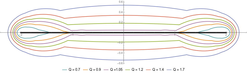
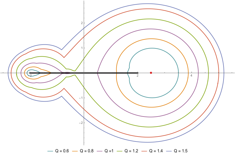
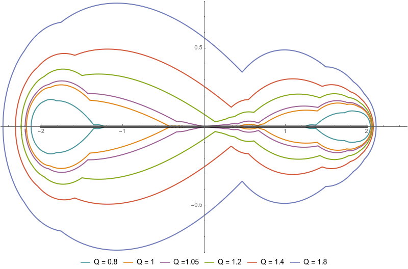
Below in Figures 3, 4 and 5, we provide illustrative plots of the optimal spectral enclosures of Theorem 3 for a∈{1/2,2,i⁡(1+5)/2}a\in\{1/2,2,{\rm i}(1+\sqrt{5})/2\}. Namely, the plots show the boundary curves given by the equation

|z2−4|=ga​(z)​Q,\sqrt{|z^{2}-4|}=g_{a}(z)Q,

for several values of the parameter Q=‖v‖ℓ1Q=\|v\|_{\ell^{1}}. For a=2a=2 and a=i⁡(1+5)/2a={\rm i}(1+\sqrt{5})/2, the spectrum of the unperturbed operator JaJ_{a} contains the extra eigenvalue a+a−1a+a^{-1}, see Theorem 1, that is designated by a red dot.
Refer to caption
Figure 3. Optimal spectral enclosures (7) for a=1/2a=1/2 and several values of Q=‖v‖ℓ1Q=\|v\|_{\ell^{1}}.
Refer to caption
Figure 4. Optimal spectral enclosures (7) for a=2a=2 and several values of Q=‖v‖ℓ1Q=\|v\|_{\ell^{1}}. The red dot designates the sole eigenvalue of JaJ_{a}.
Refer to caption
Figure 5. Optimal spectral enclosures (7) for a=i⁡(1+5)/2a={\rm i}(1+\sqrt{5})/2 and several values of Q=‖v‖ℓ1Q=\|v\|_{\ell^{1}}. The red dot designates the sole eigenvalue of JaJ_{a}.

References

  • [1] Abramov, A. A., Aslanyan, A., and Davies, E. B. Bounds on complex eigenvalues and resonances. J. Phys. A 34, 1 (2001), 57–72.
  • [2] Bagarello, F., Gazeau, J.-P., Szafraniec, F. H., and Znojil, M., Eds. Non-selfadjoint operators in quantum physics: Mathematical aspects. Wiley-Interscience, 2015. 432 pages.
  • [3] Böttcher, A., and Silbermann, B. Analysis of Toeplitz operators, second ed. Springer Monographs in Mathematics. Springer-Verlag, Berlin, 2006. Prepared jointly with Alexei Karlovich.
  • [4] Cassano, B., Ibrogimov, O. O., Krejčiřík, D., and Štampach, F. Location of eigenvalues of non-self-adjoint discrete Dirac operators. Ann. Henri Poincaré 21, 7 (2020), 2193–2217.
  • [5] Cossetti, L., and Krejčiřík, D. Absence of eigenvalues of non-self-adjoint Robin Laplacians on the half-space. Proc. London. Math. Soc. 121 (2020), 584–616.
  • [6] Dereziński, J., and Richard, S. On Schrödinger operators with inverse square potentials on the half-line. Ann. Henri Poincaré 18, 3 (2017), 869–928.
  • [7] Devyver, B., Fraas, M., and Pinchover, Y. Optimal Hardy-type inequalities for elliptic operators. C. R. Acad. Sc. Paris 350 (2012), 475–479.
  • [8] Devyver, B., Fraas, M., and Pinchover, Y. Optimal Hardy weight for second-order elliptic operator: an answer to a problem of Agmon. J. Funct. Anal. 266 (2014), 4422–4489.
  • [9] Enblom, A. Estimates of eigenvalues of Schrödinger operators on the half-line with complex-valued potentials. Oper. Matrices 11 (2017), 369–380.
  • [10] Fanelli, L., Krejčiřík, D., and Vega, L. Spectral stability of Schrödinger operators with subordinated complex potentials. J. Spectr. Theory 8 (2018), 575–604.
  • [11] Frank, R. L., Laptev, A., and Seiringer, R. A sharp bound on eigenvalues of Schrödinger operators on the half-line with complex-valued potentials. In Spectral Theory and Analysis (2011), J. Janas, P. Kurasov, A. Laptev, S. Naboko, and G. Stolz, Eds., vol. 214 of Oper. Theory Adv. Appl., Springer, Basel, pp. 39–44.
  • [12] Hansmann, M., and Krejčiřík, D. The abstract Birman-Schwinger principle and spectral stability. J. Anal. Math.. to appear.
  • [13] Ibrogimov, O. O., and Štampach, F. Spectral enclosures for non-self-adjoint discrete Schrödinger operators. Integral Equations Operator Theory 91, 6 (2019), Paper No. 53, 15.
  • [14] Kato, T. Wave operators and similarity for some non-selfadjoint operators. Math. Ann. 162 (1966), 258–279.
  • [15] Keller, M., Pinchover, Y., and Pogorzelski, F. An improved discrete Hardy inequality. Amer. Math. Monthly 125, 4 (2018), 347–350.
  • [16] Keller, M., Pinchover, Y., and Pogorzelski, F. Optimal Hardy inequalities for Schrödinger operators on graphs. Comm. Math. Phys. 358, 2 (2018), 767–790.
  • [17] Krejčiřík, D., and Štampach, F. A sharp form of the discrete Hardy inequality and the Keller–Pinchover–Pogorzelski inequality. Amer. Math. Monthly, to appear (2021).
  • [18] Kufner, A., Maligranda, L., and Persson, L.-E. The prehistory of the Hardy inequality. Amer. Math. Monthly 113, 8 (2006), 715–732.
  • [19] Mizutani, H., and Schiavone, N. M. Keller-type bounds for Dirac operators perturbed by rigid potentials. arXiv:2108.12854 [math.SP].
  • [20] Reed, M., and Simon, B. Methods of Modern Mathematical Physics, IV. Analysis of Operators. Academic Press, New York, 1978.
  • [21] Simon, B. Orthogonal polynomials on the unit circle. Part 2, vol. 54 of American Mathematical Society Colloquium Publications. American Mathematical Society, Providence, RI, 2005. Spectral theory.
  • [22] Weidl, T. Remarks on virtual bound states for semi-bounded operators. Comm. Partial Differential Equations 24, 1-2 (1999), 25–60.