Dynamic alignment and plasmoid formation in relativistic magnetohydrodynamic turbulenceJournal: ApJL
Abstract
We present high resolution 2D and 3D simulations of magnetized decaying turbulence in relativistic resistive magneto-hydrodynamics. The simulations show dynamic formation of large scale intermittent long-lived current sheets being disrupted by the tearing instability into plasmoid chains. These current sheets are locations of enhanced magnetic field dissipation and heating of the plasma. We find magnetic energy spectra , together with strongly pronounced dynamic alignment of Elsasser fields and of velocity and magnetic fields, for strong guide-field turbulence, whereas we retrieve spectra for the case of a weak guide-field.
Keywords:
Magnetohydrodynamics — Plasma Astrophysics — Relativistic Fluid DynamicsI Introduction
Turbulence provides a route for the energy cascade and dissipation in a wide range of astrophysical plasmas. This is relevant for astrophysical systems like black hole accretion disk-jet systems (Ripperda et al. 2020; Ripperda et al. 2021; Mahlmann et al. 2020, e.g.,), magnetar magnetospheres (Beloborodov 2020) and pulsar wind nebulae (Lyubarsky 1992; Begelman 1998, e.g.,). These astrophysical systems are typically relativistic, meaning that the magnetization , where is the magnetic field strength, is the plasma density, and is the relativistic enthalpy density, indicating that the magnetic energy density is larger than the plasma energy density. This results in an Alfvén speed that is close to the speed of light .
Most turbulence studies have been in the realm of non-relativistic magnetohydrodynamics (MHD) when the Alfvén speed, , is much lower than the speed of light, . Iroshnikov 1963; Kraichnan 1965 showed that the energy cascade from large to small scales is caused by the mutual shear of counter-propagating Alfvén waves. Thirty years later Goldreich & Sridhar 1995; Goldreich & Sridhar 1997 suggested that turbulent systems are in the critical balance regime meaning that an eddy is significantly deform ed during one Alfvén-crossing time. This also means that the turbulent eddies are elongated along the background magnetic field. The first steps towards a theory of relativistic turbulence were taken recently by Chandran et al. 2018, and they demonstrated that the relativistic picture is very similar to the Newtonian limit ( more details are presented in Section II). Boldyrev 2005; Boldyrev 2006 suggested that turbulent eddies are anisotropic in all three directions: they are elongated along the guide magnetic field and have two different sizes in the guide field-perpendicular plane. The ratio of these two sizes is called dynamic alignment angle. These eddies are progressively more elongated at smaller scales. Recent theories (Boldyrev & Loureiro 2017; Mallet et al. 2017, e.g.,) proposed that the elongated eddies at small enough scale become unstable to the tearing instability, causing a steepening of the turbulence spectrum.
In their recent paper, Dong et al. 2018 demonstrated the formation of reconnecting current sheets in two-dimensional (2D) decaying non-relativistic turbulence. They also demonstrated the formation of a turbulence spectrum and dynamic alignment in agreement with Boldyrev’s theory. It is however as of yet unclear whether these findings persist in the case of realistic three-dimensional (3D) turbulence. In 3D MHD, despite prominent current sheet formation (Zhdankin et al. 2013), it remains unclear whether reconnection can occur in the fast regime, when the dissipation efficiency is independent of resistivity. This regime is associated with the formation of plasmoid chains, resulting in a universal reconnection rate of order (Bhattacharjee et al. 2009; Uzdensky et al. 2010).
Plasmoid-mediated reconnection in relativistic plasmas can accelerate particles to non-thermal energies (e.g., Sironi & Spitkovsky 2014; Guo et al. 2014; Werner et al. 2015), responsible for the high-energy emission in many environments of compact objects (e.g., Cerutti et al. 2015; Beloborodov 2017). Recent studies of relativistic turbulence in collisionless plasmas have shown efficient particle acceleration (Zhdankin et al. 2017; Comisso & Sironi 2018) and the formation of reconnecting current sheets, which are important for the process of initial particle acceleration (Comisso & Sironi 2018) both in 2D and 3D. The high-energy power-law tail of the distribution function has been shown to get steeper quickly for smaller ratios of the turbulent component of the field to the guide field at the outer scale, . This observation further motivates the exploration of current sheet properties at moderate , when particle acceleration is efficient.
The highly magnetized relativistic () MHD limit has been largely unexplored, and it is unclear whether dynamic alignment forms in this regime, and whether it plays an important role for the current sheet formation for situations where . Neither any presence of dynamic alignment nor plasmoid unstable current sheets were shown in the first relativistic ideal MHD simulations by Zrake & MacFadyen 2012.
In this Letter we present numerical relativistic resistive MHD simulations of decaying turbulence in highly-magnetized plasma both in 2D and 3D. We demonstrate that dynamic alignment forms both in 2D and 3D. We show intermittent long-lived current sheets form naturally in the turbulence and become plasmoid-unstable.
II Theoretical overview
The study of non-relativistic turbulence is usually done with a reduced MHD approach. This method employs a few assumptions: a uniform, strong, in comparison to the perturbation , guide field and incompressibility of the flow (, where is the sound speed). Under these assumptions, the only waves of interest are perpendicularly-polarized Alfvén waves, propagating along the guide field. The reduced form of MHD equations in this limit reads (Elsasser 1950):
| (1) |
where is the total pressure, and are the Elsasser fields, representing counter-propagating Alfvén waves.
The ideal relativistic MHD equations consist of mass and stress-energy conservation laws, and the induction equation for the magnetic field evolution:
| (2) |
Here are 4-dimensional space-time indices, such that is the four-velocity vector, is Lorentz factor, and is the stress-energy tensor
| (3) |
with and is the relativistic enthalpy, , the flat-spacetime Minkowski metric. is the magnetic field four-vector
| (4) |
and . Introducing the relativistic Elsasser fields
| (5) |
and modified pressure term, , one can rewrite the relativistic MHD equations in the Elsasser-type form: (Chandran et al. 2018; TenBarge et al. 2021)
| (6) |
In contrast to the non-relativistic case, one cannot formally introduce an incompressible limit in relativistic MHD wherein there is a maximum speed of propagation, . The finite speed of light prevents easy elimination of the fast magnetosonic modes (Takamoto & Lazarian 2017). However, it is still possible to order them out in the highly anisotropic limit, , which implies , where and are the frequencies of the fast magnetosonic and Alfvén modes, correspondingly (TenBarge et al. 2021). Here, we are interested in the highly-magnetized limit, where the hot magnetization parameter, , is large:
| (7) |
This implies , or , and the elimination of the slow magnetosonic mode. The second term of the relativistic Elsasser variable is a unit vector in the direction of the four-magnetic field vector as in this limit.
TenBarge et al. 2021 discusses the Elsasser-type equations of the relativistic MHD in the highly anisotropic limit, , constructed in the average fluid rest frame (Chandran et al. 2018). In three-vector form the result is particularly similar to the reduced non-relativistic MHD equations:
| (8) |
Due to the close resemblance between the Newtonian and relativistic set of reduced MHD equations, once the anisotropic cascade reaches sufficiently small scales, where is satisfied, one can expect that relativistic MHD turbulence is statistically similar to its Newtonian counterpart. In the case of interest, , the last term of (8) is negligible, and the Alfvén speed is close to the speed of light, , such that the equations are particularly simple:
| (9) |
The applicability of equation (9) is limited to regimes where . However, when plasma is heated to relativistic temperatures, e.g., in reconnection layers, this assumption is not justified, at least locally. Since there is no a formally incompressible limit in relativistic systems, and our interest in systems with , which is particularly challenging to explore analytically, we turn to numerical simulations to confirm these expectations.
An important feature of the highly magnetized MHD turbulence is the overall dominance of the magnetic and electric field fluctuations, , over the kinetic energy, . This can be seen from the following relations for a single Alfvén wave in the relativistic regime ():
where the inequality is used,
| (10) |
Current sheets are important dissipative structures in magnetized turbulence, and it is useful to compare their behavior in non-relativistic and relativistic regimes. In a near-stationary current sheet, the reconnection rate is the ratio of the inflow velocity to the outflow velocity (Parker 1957; Sweet 1958). If the plasma can be assumed incompressible, it then follows that where is the thickness and is the length of the current sheet. The thickness of a Sweet-Parker current sheet is determined from continuity of the resistive and ideal electric fields as , where is the resistivity. The outflow speed can be approximated as the Alfvén speed , which in a relativistic plasma is . This results in a relativistic reconnection rate of , i.e., a result identical to the non-relativistic case (Lyubarsky 2005). The reconnection rate in a Sweet-Parker sheet then scales as , where is the Lundquist number. For large Lundquist numbers, typical in astrophysical sources, reconnection is mediated by the plasmoid instability, which in non-relativistic settings gets triggered at , leading to a saturation of the reconnection rate at (Loureiro et al. 2007; Bhattacharjee et al. 2009). It was shown semi-analtyically and numerically, by solving the full set of resistive relativistic MHD equations, that this result holds for highly magnetized relativistic plasmas (Del Zanna et al. 2016; Ripperda et al. 2019).
Since magnetic field fluctuations dominate over kinetic energy, resistive dissipation dominates over viscous dissipation in the inertial range of turbulence. We show that resistive dissipation in highly-magnetized MHD plasmas is also dominant in the exhausts of reconnection layers. One can see this by comparing the rate of resistive energy dissipation , to the rate of viscous dissipation , where is the viscosity, is the kinetic energy in the exhaust region, is magnetic energy and is the typical width scale in the exhaust region. The ratio of resistive to viscous dissipation rates is then 11 1 Our argument is applicable for the case of a scalar viscosity , i.e., independent of the gas pressure which is high in the exhaust region. Whether this assumption is accurate for the effective viscosity of a collisionless relativistically hot plasma is an interesting question for further investigation.. In a non-relativistic plasma, this ratio is always of order since and . However, in highly magnetized relativistic plasma, (Lyubarsky 2005) while , and hence the ratio between resistive and viscous dissipation rates is proportional to such that resistive dissipation dominates.
III Numerical Method and Setup
We solve the set of special relativistic resistive MHD (SRRMHD) equations with the Black Hole Accretion Code (BHAC, Porth et al. 2017; Olivares et al. 2019) and an Implicit-Explicit (IMEX) time stepping scheme to evolve the stiff resistive Ohm’s law (Ripperda et al. 2019; Ripperda et al. 2019). We employ a constant and uniform resistivity , which provides the simplest prescription to allow resolved magnetic reconnection.
The SRRMHD equations are numerically evolved in a periodic domain of size in 2D and in 3D. We initialize an out-of-plane (in the -direction) guide magnetic field and an in-plane () magnetic field perturbation :
where , , and are random phases. We set initial waves in each direction for 2D runs (64 initial modes) and for 3D runs, in order to allow for a larger inertial range in 3D simulations. The outer (or energy containing) scale is then for 2D simulations and for 3D. The turbulence at smaller scales forms self-consistently via energy cascading. In 3D we modulate with two modes , where is also a random phase. The normalization coefficient is then . We initialize the plasma at rest, with velocity field , and with a uniform gas pressure and rest mass density . We set an adiabatic index , assuming an ideal relativistic gas. Similar initial conditions for the magnetic field were employed in relativistic particle-in-cell (PIC) (Comisso & Sironi 2018; Nättilä & Beloborodov 2020) turbulence simulations. For all simulations we set .
In order to characterize the strength of both the guide and the in-plane magnetic field we introduce two magnetization parameters
| (11) |
A summary of the performed runs is given in Table 1. We employ an elongated box with for run 3D[d] to enforce the critical balance condition at the outer scale.
| Sim | Res | Grid | ||||
|---|---|---|---|---|---|---|
| 2D[a] | 5 | 5 | AMR | |||
| 2D[b] | 5 | 5 | AMR | |||
| 2D[c] | 5 | 5 | AMR | |||
| 2D[d] | 1 | 1 | AMR | |||
| 2D[e] | 1 | 5 | AMR | |||
| 2D[f] | 5 | 5 | Uni | |||
| 3D[a] | 1 | 5 | Uni | |||
| 3D[b] | 5 | 5 | Uni | |||
| 3D[c] | 1 | 1 | Uni | |||
| 3D[d] | 9 | 1 | Uni |
We set the resistivity to either in the 2D setup, which corresponds to Lundquist numbers for the largest current sheets of length , and . The simulation with is well-above the critical Lundquist number limit , while the simulation with is approximately at the limit . Potentially, current sheets can become plasmoid unstable at a smaller critical Lundquist number in a turbulent flow (Loureiro et al. 2009). We explore whether this effect is significant in 2D relativistic turbulence with our simulation.
In order to ensure that the resistive length scales are resolved, and results are converged with numerical resolution, we develop a novel adaptive mesh refinement (AMR) strategy (see Appendix A). We benchmark our 2D results with a short simulation (until ) on a uniform grid, with a resolution of . In 3D it is impossible to fully converge due to numerical limitations, and instead we employ the highest feasible resolution that allows to capture the development of the plasmoid instability in the longest current sheets. One high-resolution run is performed with grid points to probe the formation of plasmoid chains. We additionally present a study with different values of the magnetization parameter at a resolution of grid points.
The SRRMHD algorithm relies on viscosity at the grid level, such that the magnetic Prandtl number for 2D simulations, and for 3D simulations with a marginally resolved resistive scale, assuming resistive and viscous scales are similar and governed by the finite grid resolution. This choice is further motivated by the fact that viscous effects are subdominant for highly-magnetized plasmas, as we have demonstrated in Section II.
IV Results
We present the results of simulations which we run until , such that the turbulence is fully developed and settles to a quasi-steady state. For the case of decaying turbulence considered in this Letter, we define a quasi-steady state when the spectral slope is constant for at least one outer scale eddy turnover time, , while the total energy dissipates. Here, is the amplitude of the Fourier mode of the magnetic field with wavenumber . It takes for the energy to cascade from the initial low modes to the resistive scale. At the spectrum flattens until it reaches a quasi-steady state. This behavior of the power spectrum is illustrated in the attached video22 2 Direct link: https://youtu.be/n7SZigrJ9kk . In order to test convergence of the simulation, we compare spectra of magnetic energy, , for different resolutions: if the onset of the inertial range cutoff does not change with increasing resolution (the vertical lines in Figure 5c), i.e., if the cutoff is determined by the resolved resistive scale, the simulation is considered converged. More details about the AMR strategy and convergence tests are presented in the Appendix A.
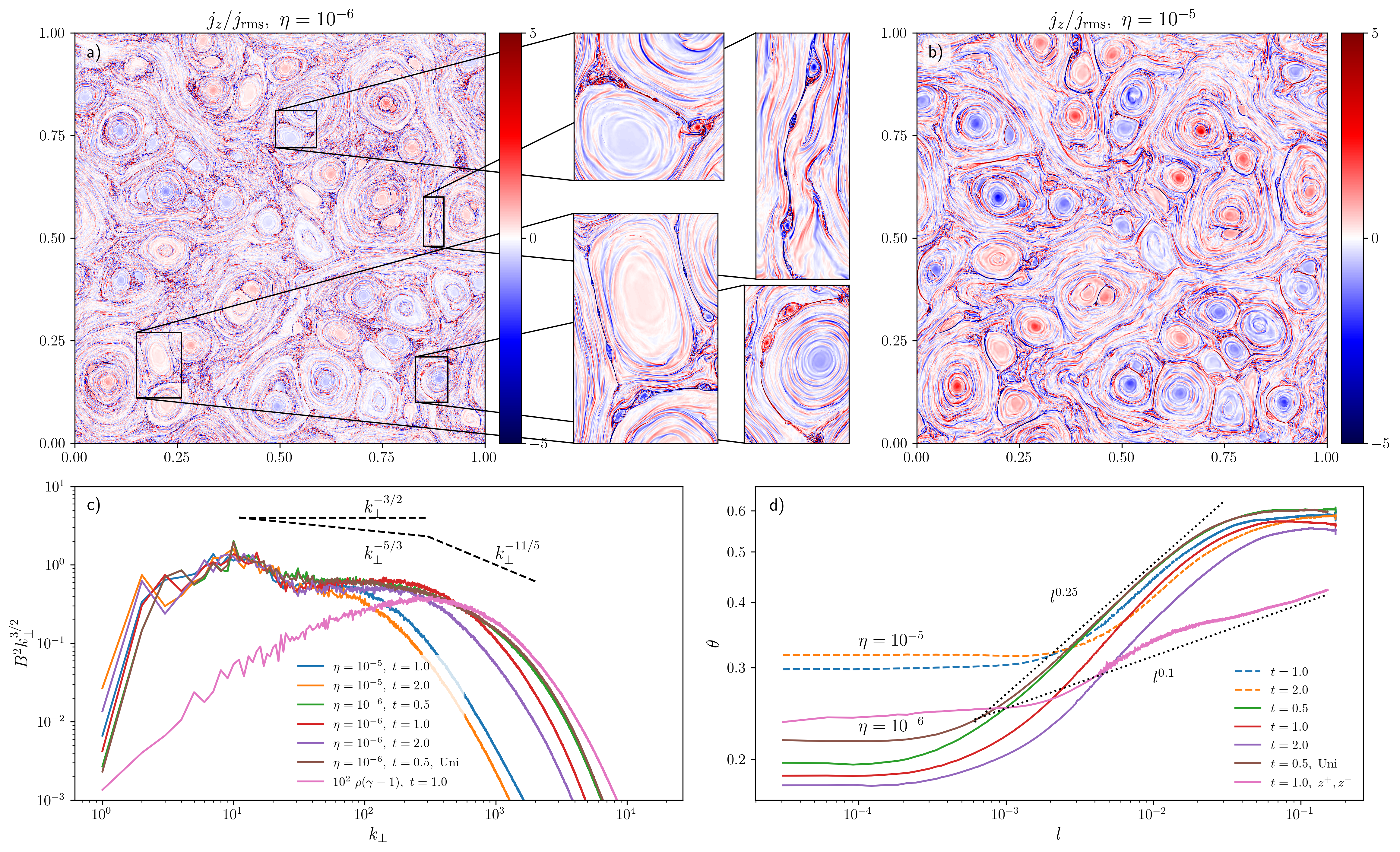
In Figure 1a we present the distribution of the out-of-plane electric current density for a 2D simulation with an effective resolution of grid points, 2D[a], and 3 AMR levels, for a resistivity . Here, we set magnetizations , equivalent to a total magnetization . Very long current sheets emerge at the interfaces of large merging eddies. The length of a current sheet is mainly defined by the size of the largest eddies present in the system. Estimating the length of these current sheets as and accounting for the relativistic Alfvén speed , we find the Lundquist number to be . These current sheets are plasmoid-unstable and break up into current sheets of smaller length scales, such that their Lundquist numbers . This results in a maximum number of plasmoids, which is consistent with results shown in Figure 1a. We also perform simulations for and and resistivity . Plasmoid-unstable current sheets form ubiquitously for all of these settings. For resistivity we observe only few plasmoids (for the longest current sheets) in the whole domain indicating that the critical Lundquist number holds for the plasmoid instability in current sheets in a 2D turbulent flow. By varying numerical resolution, we find that the onset of the plasmoid instability occurs at lower resolution for the cases with weaker guide field, , motivating our choice to perform our highest resolution 3D simulation for (run 3D[a]).
2D and 3D weak guide field (3D[a]) simulations show pronounced reconnection-mediated mergers of smaller eddies. This process has also been recently observed in simulations of merging non-helical flux tubes (Zhou et al. 2020). Our very long 2D simulations with a (smaller) resolution of demonstrate that the terminal state of the turbulence has two large eddies of opposite magnetic helicity remaining in the simulation box. 3D simulations show similar behavior. In order to identify current sheets, we choose a threshold in the current density, , and consider a point to be in the current sheet if , where is the root-mean-square of the electric current in the domain (Zhdankin et al. 2013). The long current sheets have an intermittent nature and occupy about 0.2-0.5 of the domain in 2D, yet they are responsible for of the magnetic field dissipation, , for . Our results are insensitive to the exact value of , as long as . For a larger value of resistivity, , only few plasmoids form in the whole simulation box (see Figure 1b). Comparing to the case, the current sheets for are thicker and, hence, have a lower current density amplitude. In this case we find only of the dissipation to happen in the localized current sheets.
The anisotropic properties of the turbulence can be quantified by measuring the dynamic alignment angle of eddies in the plane perpendicular to the guide field (Boldyrev 2005; Boldyrev 2006). We employ a Monte-Carlo method to compute dynamic alignment angle as a function of a point-separating vector. Following the method proposed by Mason et al. 2006; Perez et al. 2012, we compute two structure functions , , where and are increments of the velocity and the magnetic field perpendicular to the local guide field at scale . The alignment angle is defined as
| (12) |
where and are sizes of the eddy in the guide field-perpendicular plane. Note that both and are first order structure functions , and one can define the alignment angle for any as . It turns out that the slope of the alignment angle function is dependent on the order of the structure function (Mallet et al. 2016) revealing the intermittent nature of dynamic alignment (Frisch 1995). We present more details on the intermittency of dynamic alignment in Appendix C.
The slope of the dynamic alignment angle as a function of the size of eddies is tightly connected to the power-law of the magnetic energy spectrum, , which is predicted to be for turbulence that is anisotropic in the plane perpendicular to the guide field (Boldyrev 2006). By introducing a non-linear time, (Boldyrev 2005), we can relate the power spectrum with the alignment angle:
| (13) | ||||
where is the energy cascading rate, is the increment of the magnetic field at a scale in the plane perpendicular to the guide field. For , it reproduces Boldyrev’s spectrum . In the case of no alignment being present, , it reduces to the Goldreich & Sridhar 1995 spectrum, .
In Figure 1c we show the magnetic power spectrum in the steady state and multiply the result by , to make the difference between the power law indices and more pronounced. Figure 1c clearly demonstrates that the spectrum is closer to in the inertial range. We define the steady state of decaying turbulence when the spectral slope is constant in time, at , allowing us to compare our results with steady state theory. Note that the total energy decreases in time while the normalized spectrum , which we present in all spectrum plots, is constant in time. It is worth mentioning that in non-relativistic reduced MHD simulations one typically analyzes the spectrum of the total kinetic and magnetic energy (Perez et al. 2012). In our highly magnetized relativistic simulations however, , and we confirmed that the contribution of the kinetic energy is negligible for both 2D and 3D simulations (see spectra in Figures 1c and 2c). To preserve the kinetic to magnetic field energy ratio, we also normalize the kinetic energy by . In agreement with the power spectrum, the dynamic alignment (Figure 1d) demonstrates a perfect match with Boldyrev’s prediction, , at the intermediate scales, , where is defined by the number of modes in the initial conditions, and is defined by the resistive scale.
Chandran et al. 2015 proposed that mutual shear of counter-propagating Elsasser fields is responsible for the dynamic alignment. They predict that these two fields create a progressively decreasing alignment angle, while the slope becomes flatter. To test this hypothesis, we measure the alignment angle between two Elsasser fields:
| (14) |
Straightforward application of the non-relativistic Elsasser field expression, , results in , while , giving that their ratio in highly magnetized plasma. However, one should use the relativistic formulation of Elsasser fields (5) in this regime, where and can be comparable. The dynamic alignment angle between the relativistic Elsasser fields is flatter than at , for (Figure 1d). The average slope is close to the result, as predicted by Chandran et al. 2015, although it displays an unexpected break at intermediate scales.
The smallest averaged dynamic alignment angle, , in the simulation with is , and it is approximately constant for small scales. Deviations from Boldyrev’s scaling are visible at scales where resistive effects become important. Note that this is also where the inertial range of the spectra ends. The plasmoid-unstable current sheets we observe in the simulation possess much smaller alignment angles , in accordance with Loureiro et al. 2007. The presence of such current sheets with alignment angles of an order of magnitude smaller than the minimal averaged alignment angle that we find, implies the intermittent nature of these sheets (Dong et al. 2018). Formation of intermittent plasmoid-unstable current sheets can be responsible for a steepening of the spectrum at the end of the inertial range, which we observe in the range at in Figure 1c. However, we assume that the scale separation in our simulations is not enough to robustly confirm the prediction by Boldyrev & Loureiro 2017 and Mallet et al. 2017 for the non-relativistic reconnection-mediated regime. We also do not observe the increase of the alignment angle at small scales corresponding to wave-vectors in the steepening range, as predicted in Boldyrev & Loureiro 2017.
Since the onset of the plasmoid instability occurs at lower resolution in 2D simulations if a weaker guide field is assumed, we run a 3D simulation (3D[a]) with , , and highest resolution of grid points. For 2D simulations we confirm that full plasmoid chains form for smaller values of as well, but higher resolutions are required to resolve the instability. We refer to the case with initial (run 3D[a]) as a weak guide field, and to the case with initial (run 3D[d]) as a strong guide field. We note that by , when we analyze the simulations, the turbulent component of the field decayed to (3D[a]) and (3D[d]).
For the strong guide field case, the energy cascade is developing mainly in , and the full 3D analysis can be reduced to a 2D analysis in a set of planes (Perez et al. 2012, e.g.,). For simplicity, in the case of the weak guide field we also compute the spectrum for wavevectors perpendicular to using the same method (a more accurate calculation would use structure functions which take into account a locally varying guide field, Cho & Vishniac 2000). In order to provide a statistically significant result, we average the 2D spectrum and dynamic alignment angle in the set of planes taken at various . We confirm that the spectrum and the alignment angles are independent of the choice of the sampling planes if , where is the number of grid points in the direction along .

We consider the turbulence at to be in a steady state, i.e., the dynamic alignment is fully formed (see Figure 2). We confirm the steady state shape of the dynamic alignment angle function beyond with longer simulations at a lower numerical resolution, (runs 3D[b], 3D[c]). The slope of the alignment angle is close to the predicted for the smaller eddies and is less pronounced for eddies of the system size scale (see Figure 2d). In simulation 3D[a] with the initially weaker guide field , at , the alignment angle curve is significantly shallower, consistent with the steady state in driven non-relativistic turbulence at (Mason et al. 2006). At this time, the strength of turbulent fluctuations is similar to the strength of the guide field, . Further dissipation of the magnetic energy leads to at , and a steeper alignment angle curve. The spectrum of the turbulence develops simultaneously with the dynamic alignment.
The slope of the dynamic alignment angle, , is comparable to for the strong guide field (run 3D[d], , ). For the weak guide field (3D[a], , ), the alignment is very weakly pronounced. At the same time, the slope of the energy spectrum of 3D[a] is closer to as predicted by Goldreich-Sridhar theory with no dynamic alignment. It could be considered as an indication that the dynamic alignment of Elsasser fields rather than the one of reduces the non-linearity.
3D simulations show less pronounced boundaries of large-scale eddies, but the intermittent large current sheets are still present in the system with the weak guide field. Figure 2a and the linked video33 3 Direct link: https://youtu.be/nY3F4bnTtEM demonstrate the distribution of the electric current in the planes perpendicular to the guide field, , at , and Figure 2b and the accompanying video44 4 Direct link: https://youtu.be/8CRiWAZg_Bo show the same at . Similarly to the 2D results, intense current sheets occupy up to of the total volume of the domain55 5 The larger filling fraction in 3D simulations is potentially attributed to the fact that for a similar value of resistivity, , the widths of current sheets are not fully converged. and lead to of the total dissipation of the magnetic energy. Intermittent long current sheets are clearly plasmoid-unstable as shown by the insets in Figure 2. A few initial eddies are still clearly seen at , but many long intermittent current sheets are unaffected by the choice of the initial conditions. At no visible features are associated with the initial conditions (see Figure 2b).
Overall, the structure of the electric current in the 3D weak guide field simulation looks similar to the one in 2D (Figure 1a): there is a number of well-pronounced long, plasmoid unstable current sheets formed at the outer scale. Their formation is likely associated with the mergers and subsequent reconnection of large coherent structures (Hosking & Schekochihin 2020). Unlike in the weak guide field regime, the strong guide field simulation 3D[d] shows the statistical properties of “aligned” critically-balanced turbulence: the spectrum and a pronounced dynamic alignment (dashed lines in Figure 2c and d). The spatial distribution of the electric current is more uniform in this case (see Figure 3). The absence of very long current sheets is consistent with the observation of a very few plasmoids in the simulation (see insets of Figure 3). A possible explanation can be found in the small ratio of the length, , for the sheets shown in the insets of Figure 3, to the width of these sheets, which at our resolution is still limited by the numerical diffusion. We anticipate that the plasmoid instability can be more reliably captured at much higher spatial resolution: for the typical length, , and the width-to-length ratio , one requires grid points, where cells is the minimally desired resolution per width of the plasmoid-unstable current sheet.

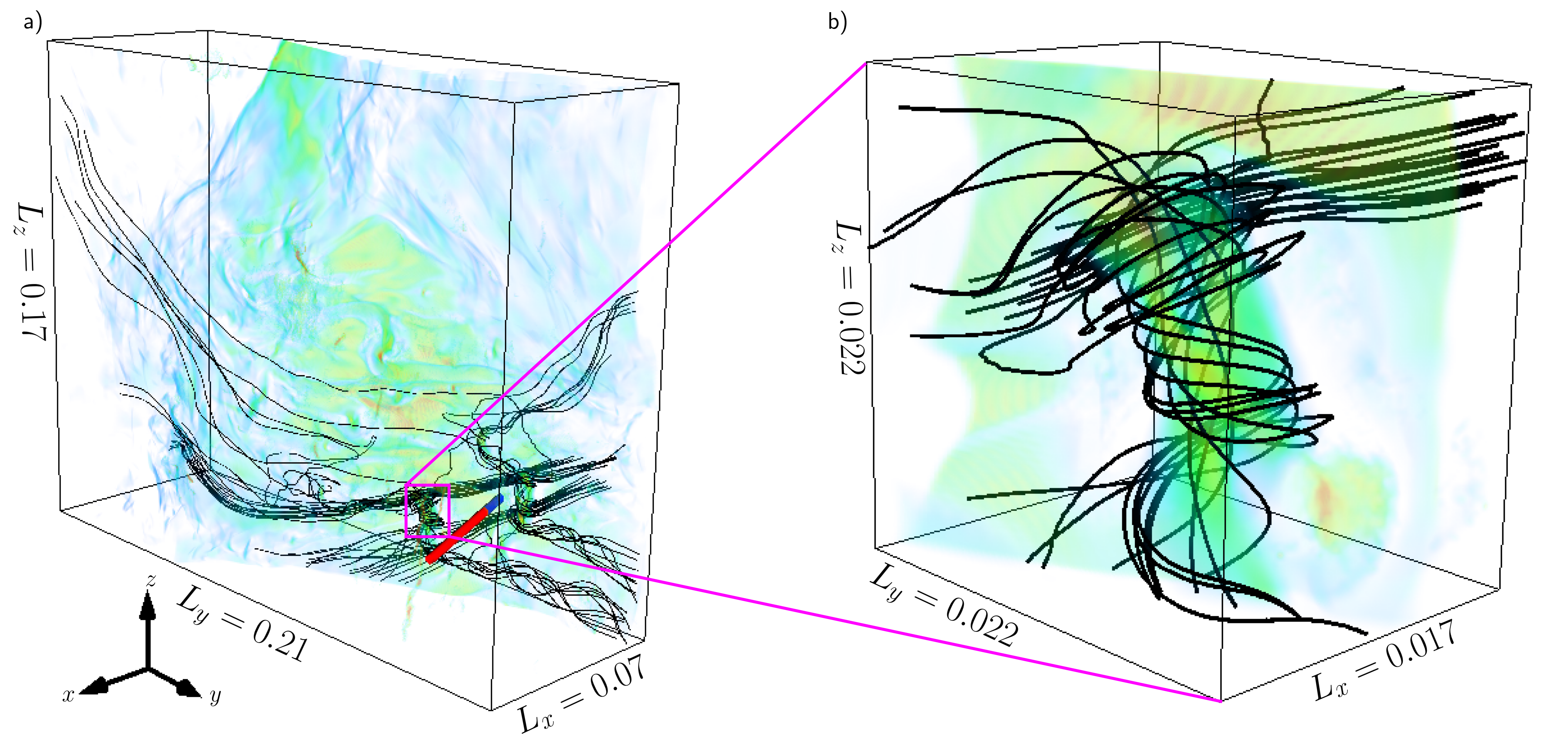
The structure of a representative current sheet for the weak guide field simulation 3D[a] is presented in Figure 4. The volume render represents the current density amplitude, and solid black lines show selected magnetic field lines. The lower threshold for the volume rendering is chosen to be , in order to remove the upstream regions without significant current. The initial (seed) points for the integration of magnetic field lines are set inside two randomly chosen plasmoids. Wrapped, helical magnetic field is responsible for the large current density inside the plasmoids. The helical structure allows longer plasmoids (or, flux tubes) to be kink-unstable if their length is large enough to exceed the Kruskal-Shafranov stability limit. This instability likely limits the life time of plasmoids in current sheets and their axial extension. A zoom into the 3D structure of a plasmoid is shown in Figure 4b.
Acceleration of the flow from the X-point of a Sweet-Parker current sheet up to Alfvénic speed creates a velocity shear, which may become unstable to the Kelvin-Helmholtz instability (KHI). The analytical non-relativistic stability criterion (Loureiro et al. 2013) suggests that the strong upstream magnetic field can lead to the stabilization of the KHI for the velocity shear and the Alfvén speed determined by the upstream magnetic field strength. A similar criterion was derived for a simplified model with in a fully relativistic case (Osmanov et al. 2008). Thus, we expect current sheets in highly-magnetized turbulence to be stabilized by the strong upstream magnetic field. To confirm this prediction, we conduct localized numerical experiments with conditions inferred from turbulence simulations (see Appendix B for the description of the setups) that confirm that long plasmoid-unstable current sheets are Kelvin-Helmholtz-stable both in 2D and 3D simulations.
V Conclusions
In this Letter we present the first 2D and 3D numerical SRRMHD simulations of highly magnetized decaying turbulence. We calculate statistical properties of the turbulence, by analyzing a quasi steady state at two Alfvén-crossing times of the simulation box. We show that the spectrum of magnetic energy in both cases is close to Boldyrev’s spectrum, , and the dynamic alignment angle follows an dependence. Despite the dynamic alignment angle of and fields in 2D is perfectly following Boldyrev’s prediction, its formation cannot be explained by the uncertainty principle originally employed by Boldyrev 2006. On the other hand, intermittent structures are vastly present in the simulations, favoring the theory of mutual shearing of Elsasser fields by Chandran et al. 2015 : an in-depth analysis of this approach is presented in Appendix C. We demonstrate that long-lived intermittent current sheets form dynamically throughout the evolution. These sheets are plasmoid unstable and KH-stable. They occupy a very small fraction of the numerical domain but provide a significant fraction of the total magnetic field dissipation.
In our simulations we only employ explicit resistivity while viscosity is dictated by the finite grid resolution. We expect that the magnetic energy dominates the kinetic energy at all scales, and dissipation is governed by resistivity. It will be useful to perform simulations with explicit viscosity and fixed magnetic Prandtl number in the future studies, and to consider the trans-relativistic regime, . These studies can be applied to turbulence in the accretion disk-jet boundary with moderate magnetization (Ripperda et al. 2020).
In order to study the properties of intermittent current sheets in a statistical steady state, it is important to study driven turbulence in highly magnetized plasmas . High magnetization leads to efficient heating of the plasma due to the dissipation of magnetic energy and a significant drop of . To mediate the effect of runaway heating, radiative cooling of the plasma should be incorporated in the simulations (Zhdankin et al. 2021).
The limitation of computational resources does not allow to reach numerical resolutions significantly above in the nearby future. This is too low to reach alignment angles substantially below at the smallest scales. On the other hand, the intriguing similarity of statistical properties of 2D and 3D turbulence in our simulations makes it interesting to perform even higher resolution simulations of 2D turbulence. The most significant milestone will be a resolution of which allows progressively elongated eddies to reach an alignment angle corresponding to the plasmoid instability of these eddies. The steepening of the turbulence spectrum due to the onset of the plasmoid instability in intermittent current sheets (or due to the linear tearing instability in elongated eddies, Boldyrev & Loureiro 2017) can be measured reliably at resolutions of , realistically attainable in the nearby future, in particular with the AMR criterion we propose here.
VI Acknowledgements
We acknowledge useful discussions with Lev Arzamasskiy, Amitava Bhattacharjee, Benjamin Chandran, Luca Comisso, Mikhail Medvedev, Joonas Nättilä, Jason TenBarge, James Stone, and help in navigating through 3D-visualization by Hayk Hakobyan. The authors acknowledge insightful comments by the anonymous referee which helped to significantly improve the manuscript. The computational resources and services used in this work were provided by facilities supported by the Scientific Computing Core at the Flatiron Institute, a division of the Simons Foundation; and by the VSC (Flemish Supercomputer Center), funded by the Research Foundation Flanders (FWO) and the Flemish Government – department EWI. A.C. gratefully acknowledges support and hospitality from the Simons Foundation through the pre-doctoral program at the Center for Computational Astrophysics, Flatiron Institute. B.R. is supported by a Joint Princeton/Fellowship Postdoctoral Fellowship. A.P. acknowledges support by the National Science Foundation under Grant No. AST-1910248.
Software: BHAC, (Porth et al. 2017; Olivares et al. 2019; Ripperda et al. 2019), Python (Oliphant 2007; Millman & Aivazis 2011), NumPy (van der Walt et al. 2011), Matplotlib (Hunter 2007), Mayavi (Ramachandran & Varoquaux 2011)
Appendix A Adaptive Mesh Refinement and Convergence Study

For the fully resolved and converged 2D simulations we present the adaptive mesh refinement (AMR) criterion we designed to accelerate the simulations and to simultaneously capture the main properties of the turbulence and dissipative structures. The main principle is that the largest eddies are resolved by many cells at low resolution. To capture the physics at smallest scales, one needs to refine the resolution in the smallest eddies, capturing both velocity and magnetic field gradients. We define the characteristic sizes of the eddies as
| (A1) |
The refinement routine is called if the size of any of the two quantities is less than a threshold value: at the point. Coefficient is chosen to be such that the threshold scale is larger than the numerical resistive scale. In the simulations we use , which is larger than the numerical resistive scale in simulations 2D[a] and 2D[c], and is the grid spacing at a given resolution. Coarsening of the grid in the numerical domain is only allowed if both quantities at a given grid point are larger than the threshold. Since the electric current density is roughly given by the gradient of the magnetic field, , regions of the large electric current density (indicating current sheets) are automatically refined. Since the inverse cascade is very pronounced in 2D simulations, AMR shows very high efficiency at early times, when the spectrum is being formed, and at later times, when small eddies merge in larger ones (see Figure 5a for ). Since the resistive scale is much larger for , the coverage by the highest resolution level does not exceed in this case.
The threshold value is tested for a resolution of grid points by comparing spectra of the magnetic field energy for uniform grid and AMR-enabled runs (where the effective resolution for the AMR runs indicates the total resolution if the whole domain were refined to the highest AMR level) at the same moment in time (see Figure 5b). Interestingly, the most accurate spectra are produced by simulations where the refinement algorithm is called only every time-steps, most likely due to less numerical noise being generated during the refining and coarsening of the grid and re-interpolation. The frequency of the refinement calls is defined to ensure that the finest structures are always located inside the refined grid block during their motion in the domain. For the bulk velocity of the fluid , and CFL number , an element of the fluid travels about cells between two calls of the refinement, while the minimum size of a refined grid is cells.
This AMR strategy does not seem to be effective in 3D simulations due to the overall low grid resolution, compared to the extreme resolutions employed in 2D: AMR automatically chooses the resolution needed to resolve all the features in the block. Since the size of all features in the flow is rather defined by the numerical resolution than by an explicit resistivity, AMR refines the whole domain up to the highest available resolution. It is impossible to find a reasonable threshold for the 2D counterpart of the highest resolution 3D run with grid points: any chosen either truncates the inertial range of the spectrum or refines the whole domain shortly after the start of the simulation. Figure 5c demonstrates that a base resolution of grid points is needed to fully resolve the resistive scale for and keep the inertial range of the turbulence unaffected by the resolution. In order to demonstrate this, we compare spectra for resolutions with points.
Appendix B Kelvin-Helmholtz Stability of Current Sheets
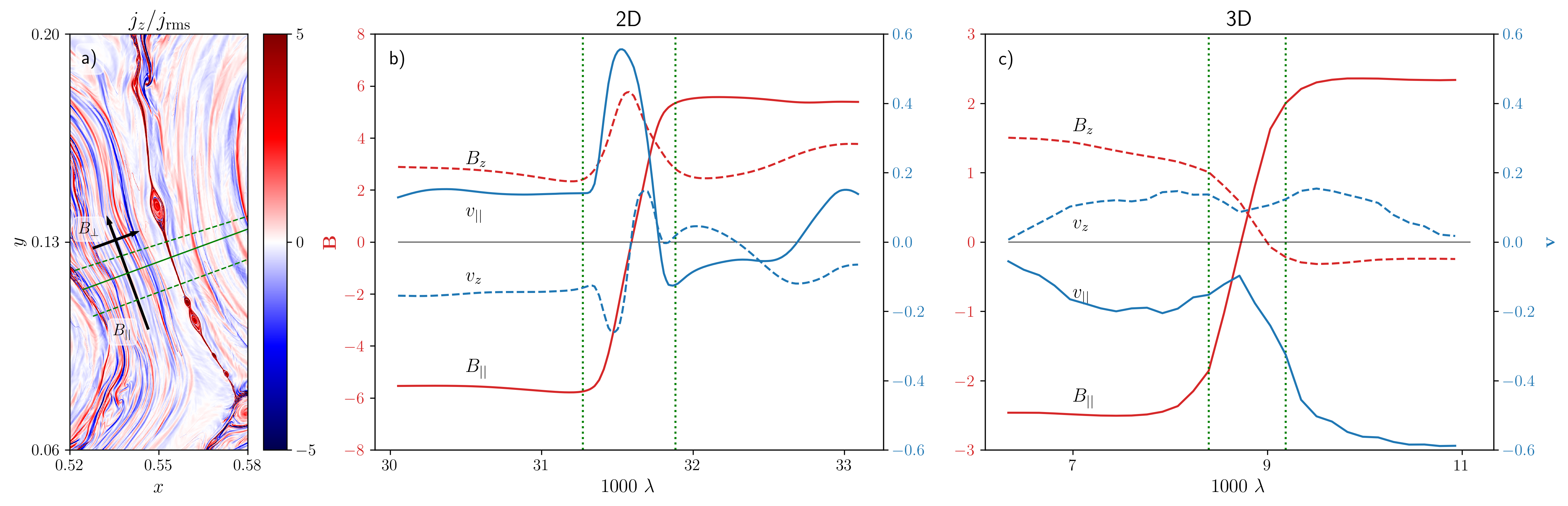
In order to study the stability of the magnetized shear flow in our plasmoid-unstable current sheets in 2D, we calculate the value of the in-plane reconnecting magnetic field component and the out-of-plane component as well as velocity field components for each of the three slices shown in Figure 6a by green lines. For all these slices we find and , where represents the direction parallel to the current sheet at a given point in the slice (the arrows in Figure 6a indicate parallel and perpendicular directions, and the -direction is out-of-plane). We show the typical behavior of these parameters in Figure 6b, which implies that the flow satisfies the non-relativistic stability criterion .
For each slice across the current sheet, we run a local simulation of the shear flow, with one flow having parameters () given by the upstream of the current sheet, and its counter-flow having parameters from the interior of the current sheet, particularly, . Zero parallel magnetic field in one of the two interacting flows prohibits reconnection at their interface in these experiments, but allows to study the KHI. Plasma pressure is adjusted to maintain the force balance across the interface of the flows.
We run simulations with a resolution of grid points for 20 light-crossing times along the sheet, which exceeds the life time of intermittent current sheets in the full 2D turbulence simulation. For the intermediate slice (shown by the solid line in Figure 6a), we run an AMR-enabled simulation with an effective resolution of grid points, which resolves all the scales up to the resistive scale for a resistivity (see Appendix A for the resolution study). This finest grid covers the whole interface of the flows at any moment of the simulation. In all of these experiments we do not observe any instability growth. This implies that the in-plane magnetic field in the upstream of the current sheet is capable of preserving KH-stability in both the upstream and downstream of the current sheet.

In order to explore the KH-stability of the 3D current sheet, we select slices between the two plasmoids (red-blue line in Figure 4), and perform test simulations in a 3D setup with a geometry similar to the one described above for 2D simulations. This slice is also normal to the surface of the current sheet at the point of their intersection. We test the sheet’s stability by running a 3D simulation with a resolution of grid points for 20 light-crossing times along the shear interface, with parameters corresponding to the slice shown in Figure 4c.
Appendix C Amplitude-dependent intermittency of the turbulence.
Since the lack of scale invariance is the most prominent sign of intermittency, we focus on the scale dependence of the Elsasser field increments, . The results presented in this Appendix are similar for as we expect the turbulence to be balanced, . As shown by Mallet et al. 2015, the scale invariance can be characterized by the similarity of the conditional probability distribution functions (PDFs) of at different scales . We computed these PDFs for 2D (run 2D[a]) and 3D (runs 3D[a] and 3D[d]) simulations. To measure the PDF, we use a set of 30 logarithmically spaced scales from to . The smallest scale , corresponding to , lies deeply in the inertial range of the energy spectrum, while the largest scale of the considered set, , is located at the outer scale of the turbulence. As the bottom row of Figure 7 shows, the smaller-scale eddies (darker lines) have higher probability to reach large normalized amplitudes of . The flattening of the PDFs at smaller scales can be attributed to the sheet-like structures emerging at these scales. For 2D and weak guide field 3D simulations, the presence of long current sheets can also explain a flatter tail of the PDF at the larger scales, while the PDF for the strong guide field 3D case has an abrupt cutoff at the high for the same eddy sizes. We normalized by a geometrical mean of at a given scale , as it is less sensitive to outliers than an arithmetical mean.
The intermittent, scale-dependent, nature of the dynamic alignment can also be shown by measuring the PDF of the dynamic alignment angle at given scales, as considered by Dong et al. 2018. We are, however, also interested in testing the assumption of Chandran et al. 2015 that large rotates into alignment, while balanced collisions are not aligned. This anti-correlation of the alignment angle with the amplitude of contradicts the intuitive explanation of the dynamic alignment by an uncertainty principle. To test this, we measure the conditional PDF of the dynamic alignment angle for a given scale and the amplitude of the Elsasser field . The middle and top rows of Figure 7 show that the the prediction is matched perfectly for strong guide field 3D turbulence: the larger , the more aligned and are. For 2D and weak guide field 3D turbulence there is a deviation from this prediction at the outer scale: while the statement holds for intermediate amplitudes of , at high amplitudes eddies become uncorrelated again. The most powerful increments are associated to current sheets and plasmoids, and one can expect that circular plasmoids have an alignment angle (the ratio of two length scales of the eddy) that can explain decorrelation of the alignment angle at high .
References
- Begelman (1998) Begelman, M. C. 1998, ApJ, 493, 291. https://arxiv.org/abs/astro-ph/9708142
- Beloborodov (2017) Beloborodov, A. M. 2017, ApJ, 850, 141, doi: 10.3847/1538-4357/aa8f4f
- Beloborodov (2020) Beloborodov, A. M. 2020, Emission of magnetar bursts and precursors of neutron star mergers. https://arxiv.org/abs/2011.07310
- Bhattacharjee et al. (2009) Bhattacharjee, A., Huang, Y.-M., Yang, H., & Rogers, B. 2009, Physics of Plasmas, 16, 112102
- Boldyrev (2005) Boldyrev, S. 2005, ApJ, 626, L37. https://arxiv.org/abs/astro-ph/0503053
- Boldyrev (2006) —. 2006, Phys. Rev. Lett., 96, 115002. https://arxiv.org/abs/astro-ph/0511290
- Boldyrev & Loureiro (2017) Boldyrev, S., & Loureiro, N. F. 2017, ApJ, 844, 125. https://arxiv.org/abs/1706.07139
- Cerutti et al. (2015) Cerutti, B., Philippov, A., Parfrey, K., & Spitkovsky, A. 2015, MNRAS, 448, 606, doi: 10.1093/mnras/stv042
- Chandran et al. (2018) Chandran, B. D. G., Foucart, F., & Tchekhovskoy, A. 2018, Journal of Plasma Physics, 84, 905840310. https://arxiv.org/abs/1707.06216
- Chandran et al. (2015) Chandran, B. D. G., Schekochihin, A. A., & Mallet, A. 2015, ApJ, 807, 39. https://arxiv.org/abs/1403.6354
- Cho & Vishniac (2000) Cho, J., & Vishniac, E. T. 2000, ApJ, 539, 273, doi: 10.1086/309213
- Comisso & Sironi (2018) Comisso, L., & Sironi, L. 2018, Phys. Rev. Lett., 121, 255101. https://arxiv.org/abs/1809.01168
- Del Zanna et al. (2016) Del Zanna, L., Papini, E., Landi, S., Bugli, M., & Bucciantini, N. 2016, MNRAS, 460, 3753, doi: 10.1093/mnras/stw1242
- Dong et al. (2018) Dong, C., Wang, L., Huang, Y.-M., Comisso, L., & Bhattacharjee, A. 2018, Phys. Rev. Lett., 121, 165101. https://arxiv.org/abs/1804.07361
- Elsasser (1950) Elsasser, W. M. 1950, Physical Review, 79, 183, doi: 10.1103/PhysRev.79.183
- Frisch (1995) Frisch, U. 1995, Turbulence: The Legacy of A. N. Kolmogorov (Cambridge University Press), doi: 10.1017/CBO9781139170666
- Goldreich & Sridhar (1995) Goldreich, P., & Sridhar, S. 1995, ApJ, 438, 763
- Goldreich & Sridhar (1997) —. 1997, ApJ, 485, 680. https://arxiv.org/abs/astro-ph/9612243
- Guo et al. (2014) Guo, F., Li, H., Daughton, W., & Liu, Y.-H. 2014, Phys. Rev. Lett., 113
- Hosking & Schekochihin (2020) Hosking, D. N., & Schekochihin, A. A. 2020, arXiv e-prints, arXiv:2012.01393. https://arxiv.org/abs/2012.01393
- Hunter (2007) Hunter, J. D. 2007, Computing in Science Engineering, 9, 90, doi: 10.1109/MCSE.2007.55
- Iroshnikov (1963) Iroshnikov, P. S. 1963, AZh, 40, 742
- Kraichnan (1965) Kraichnan, R. H. 1965, Physics of Fluids, 8, 1385
- Loureiro et al. (2007) Loureiro, N. F., Schekochihin, A. A., & Cowley, S. C. 2007, Physics of Plasmas, 14, 100703. https://arxiv.org/abs/astro-ph/0703631
- Loureiro et al. (2013) Loureiro, N. F., Schekochihin, A. A., & Uzdensky, D. A. 2013, Phys. Rev. E, 87, 013102. https://arxiv.org/abs/1208.0966
- Loureiro et al. (2009) Loureiro, N. F., Uzdensky, D. A., Schekochihin, A. A., Cowley, S. C., & Yousef, T. A. 2009, MNRAS, 399, L146, doi: 10.1111/j.1745-3933.2009.00742.x
- Lyubarsky (1992) Lyubarsky, Y. E. 1992, Soviet Astronomy Letters, 18, 356
- Lyubarsky (2005) —. 2005, MNRAS, 358, 113, doi: 10.1111/j.1365-2966.2005.08767.x
- Mahlmann et al. (2020) Mahlmann, J. F., Levinson, A., & Aloy, M. A. 2020, MNRAS, 494, 4203. https://arxiv.org/abs/2001.03171
- Mallet et al. (2015) Mallet, A., Schekochihin, A. A., & Chandran, B. D. G. 2015, MNRAS, 449, L77, doi: 10.1093/mnrasl/slv021
- Mallet et al. (2017) —. 2017, MNRAS, 468, 4862. https://arxiv.org/abs/1612.07604
- Mallet et al. (2016) Mallet, A., Schekochihin, A. A., Chandran, B. D. G., et al. 2016, MNRAS, 459, 2130, doi: 10.1093/mnras/stw802
- Mason et al. (2006) Mason, J., Cattaneo, F., & Boldyrev, S. 2006, Phys. Rev. Lett., 97, 255002. https://arxiv.org/abs/astro-ph/0602382
- Millman & Aivazis (2011) Millman, K., & Aivazis, M. 2011, Computing in Science & Engineering, 13, 9 , doi: 10.1109/MCSE.2011.36
- Nättilä & Beloborodov (2020) Nättilä, J., & Beloborodov, A. M. 2020, arXiv e-prints, arXiv:2012.03043. https://arxiv.org/abs/2012.03043
- Oliphant (2007) Oliphant, T. E. 2007, Computing in Science Engineering, 9, 10, doi: 10.1109/MCSE.2007.58
- Olivares et al. (2019) Olivares, H., Porth, O., Davelaar, J., et al. 2019, A&A, 629, A61. https://arxiv.org/abs/1906.10795
- Osmanov et al. (2008) Osmanov, Z., Mignone, A., Massaglia, S., Bodo, G., & Ferrari, A. 2008, A&A, 490, 493. https://arxiv.org/abs/0802.2607
- Parker (1957) Parker, E. N. 1957, J. Geophys. Res., 62, 509, doi: 10.1029/JZ062i004p00509
- Perez et al. (2012) Perez, J. C., Mason, J., Boldyrev, S., & Cattaneo, F. 2012, Physical Review X, 2, 041005. https://arxiv.org/abs/1209.2011
- Porth et al. (2017) Porth, O., Olivares, H., Mizuno, Y., et al. 2017, Computational Astrophysics and Cosmology, 4, 1. https://arxiv.org/abs/1611.09720
- Ramachandran & Varoquaux (2011) Ramachandran, P., & Varoquaux, G. 2011, Computing in Science & Engineering, 13, 40 , doi: 10.1109/MCSE.2011.35
- Ripperda et al. (2020) Ripperda, B., Bacchini, F., & Philippov, A. A. 2020, ApJ, 900, 100. https://arxiv.org/abs/2003.04330
- Ripperda et al. (2021) Ripperda, B., Liska, M., Chatterjee, K., et al. 2021, arXiv e-prints, arXiv:2109.15115. https://arxiv.org/abs/2109.15115
- Ripperda et al. (2019) Ripperda, B., Porth, O., Sironi, L., & Keppens, R. 2019, Monthly Notices of the Royal Astronomical Society, 485, 299–314. http://dx.doi.org/10.1093/mnras/stz387
- Ripperda et al. (2019) Ripperda, B., Bacchini, F., Porth, O., et al. 2019, ApJS, 244, 10. https://arxiv.org/abs/1907.07197
- Sironi & Spitkovsky (2014) Sironi, L., & Spitkovsky, A. 2014, ApJ, 783, L21. https://arxiv.org/abs/1401.5471
- Sweet (1958) Sweet, P. A. 1958, in Electromagnetic Phenomena in Cosmical Physics, ed. B. Lehnert, Vol. 6, 123
- Takamoto & Lazarian (2017) Takamoto, M., & Lazarian, A. 2017, MNRAS, 472, 4542, doi: 10.1093/mnras/stx2292
- TenBarge et al. (2021) TenBarge, J. M., Ripperda, B., Chernoglazov, A., et al. 2021, arXiv e-prints, arXiv:2105.01146. https://arxiv.org/abs/2105.01146
- Uzdensky et al. (2010) Uzdensky, D. A., Loureiro, N. F., & Schekochihin, A. A. 2010, Phys. Rev. Lett., 105, 235002, doi: 10.1103/PhysRevLett.105.235002
- van der Walt et al. (2011) van der Walt, S., Colbert, S. C., & Varoquaux, G. 2011, Computing in Science and Engineering, 13, 22, doi: 10.1109/MCSE.2011.37
- Werner et al. (2015) Werner, G. R., Uzdensky, D. A., Cerutti, B., Nalewajko, K., & Begelman, M. C. 2015, ApJ, 816, L8
- Zhdankin et al. (2021) Zhdankin, V., Uzdensky, D. A., & Kunz, M. W. 2021, ApJ, 908, 71. https://arxiv.org/abs/2007.12050
- Zhdankin et al. (2013) Zhdankin, V., Uzdensky, D. A., Perez, J. C., & Boldyrev, S. 2013, ApJ, 771, 124. https://arxiv.org/abs/1302.1460
- Zhdankin et al. (2017) Zhdankin, V., Werner, G. R., Uzdensky, D. A., & Begelman, M. C. 2017, Phys. Rev. Lett., 118, 055103, doi: 10.1103/PhysRevLett.118.055103
- Zhou et al. (2020) Zhou, M., Loureiro, N. F., & Uzdensky, D. A. 2020, Journal of Plasma Physics, 86, 535860401. https://arxiv.org/abs/2001.07291
- Zrake & MacFadyen (2012) Zrake, J., & MacFadyen, A. I. 2012, ApJ, 744, 32. https://arxiv.org/abs/1108.1991