Learning-Based Symbol Level Precoding: A Memory-Efficient Unsupervised Learning Approach

Consider single cell MU-MISO downlink transmission scenario where $K$ single-antenna users are served by an by $M$ BS antennas. Assuming a flat-fading Rayleigh channel $\mathbf{h}_{i}\in\mathbb{C}^{{N}_{t}\times 1}$, the received signal at the $i$-th user is expressed as

where $\mathbf{h}_{i}$, $\mathbf{w}_{i}$, ${d}_{i}$ and ${n}_{i}$ represent the channel vector, precoding vector, data symbol, phase rotation and additive white Gaussian noise for the i-th user.

Instantaneous interference is categorized into constructive and destructive [21]. As an illustration, Fig. shows the QPSK constellations diagram, where the CI area is indicated by the green region with respect to the minimum distance ($\tau$) from the decision boundaries, allowing the interfering signals to be added constructively with the symbol of interest via precoding vectors. The generic geometrical representation of the CI in Fig. shows that if the maximum angle shift ($\phi=0$) in the CI region is zero, the interfering signals overlap completely on the symbol of interest. Hence, the problem becomes a strict phase angle optimization. However, the strict phase formulation is not appealing because it leads to an additional transmission power compared to the corresponding relaxed counterpart [21]. For simplicity, we define the following variables, $\hat{\mathbf{h}}_{i}=\mathbf{h}_{i}\sum_{k=1}^{K}e^{j(\phi_{k}-\phi_{i})}\in{\mathbb{C}^{M\times 1}}$, ${\mathbf{w}}=\sum_{k=1}^{K}\mathbf{w}_{k}\in{\mathbb{C}^{M\times 1}}$, $\hat{\mathbf{h}}_{Ri}=\Re\{\hat{\mathbf{h}}_{i}\}$, $\hat{\mathbf{h}}_{Ii}=\Im\{\hat{\mathbf{h}}_{i}\}$, $\mathbf{w}_{R}=\Re\{\mathbf{w}\}$ and $\mathbf{w}_{I}=\Im\{\mathbf{w}\}$. Similarly, we also let $\bm{\Psi}=\begin{bmatrix}\hat{\mathbf{h}}_{Ri}\ \hat{\mathbf{h}}_{Ii}\ \end{bmatrix}^{T}$, $\mathbf{w}_{1}=[\mathbf{w}_{R}\ \ -\mathbf{w}_{I}]^{T}$, where $\bm{\Theta}=\begin{bmatrix}\mathbf{O}_{M}&-\mathbf{I}_{M}\\ \mathbf{I}_{M}&\mathbf{O}_{M}\end{bmatrix}\ \in\mathbb{R}^{2M\times 2M}$.

In practice, the exact channel state information (CSI) is often unknown; only the estimate is

where ${\mathbf{h}}_{i}$ is the known CSI estimates at the BS and ${\mathbf{e}}_{i}$ denotes the channel error. Given this, the robust traditional recording for the downlink MU-MISO power minimization optimization is[22]

where $\bm{T}_{i}\overset{\Delta}{=}\bar{\mathbf{W}}_{i}-\Gamma_{i}\sum_{k=1,k\neq i}^{K}\bar{\mathbf{W}}_{k}\ \forall{k}$ and $\bar{\mathbf{W}}_{i}=\mathbf{w}_{i}\mathbf{w}_{i}^{\dagger}$.

The multi-cast CI formulation of the power minimization problem for the worst-case scenario is given by [22]

For simplicity, we drop the subscripts in (4) and slit the real and imaginary parts of the constraint into two separate constraints real-valued functions as follows

where $\hat{\mathbf{e}}\overset{\Delta}{=}\begin{bmatrix}\mathbf{e}_{R}&\mathbf{e}_{I}\end{bmatrix}^{T}$ and $\hat{\mathbf{h}}=\mathbf{h}_{R}+j\mathbf{h}_{I}+\mathbf{e}_{R}+j\mathbf{e}_{I}$. Then (5) becomes

We begin by unfolding (10) using an IPM ‘log’ barrier function and transform it to its equivalent unconstrained sequence of sub-problems per user[14]

where ${B}(\cdot)\triangleq-\sum\ln{(\cdot)}$ is the logarithmic barrier function, $\upsilon$ is the Lagrangian multiplier for inequality constraints. The learning framework is derived by defining a proximity operator of (11) [14]

where $\gamma\in\{0,+\infty\}$ is the training step-size, $\mathbf{w}_{0}$ is the initial precoding vector and $\upsilon$ is the Lagrange multiplier of the inequality constraint.

Intuitively, we can form NN cascade layers from (21) as follows

where $\textbf{1}\in\mathbb{R}^{1\times 2M}$ is a vector of ones. By letting $\mathbf{W}_{l}=\mathbf{I}_{2M}-2\gamma^{[l]}$, $\mathbf{b}_{l}=\gamma^{[l]}\lambda^{[l]}\textbf{1}^{T}$ and $\bm{\Xi}_{l}=\text{prox}_{\gamma^{[l]}{\upsilon}^{[l]}{B}}$, the l-layer network $\mathcal{L}^{[l-1]}\cdots\mathcal{L}^{[0]}$ will correspond to the following

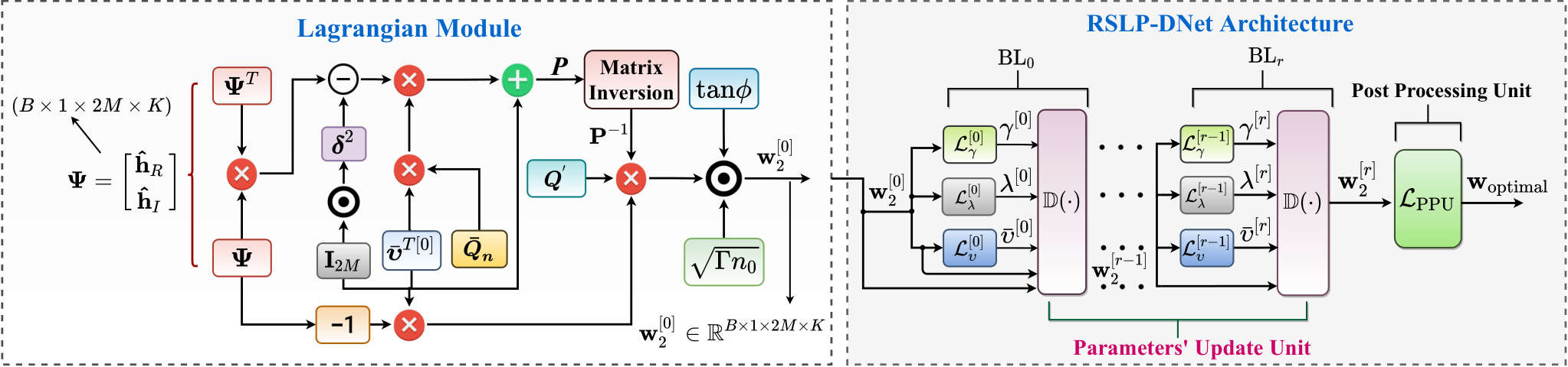
$\mathbf{W}_{l}$ and $\mathbf{b}_{l}$ present weight and bias parameters, respectively, and $\bm{\Xi}_{l}$ describes the nonlinear activation functions. Finally, based on this formulation, RSLP-DNet is built as shown in Fig. 2 and its internal DNN designs are summarised in Tables I and II.

Traditionally, DNN is designed with full-precision weights and activations. The quantization schemes have been proposed to design low-bit DNN models to address the problems of limited storage capacity and reduce hardware requirements during model deployment.

The RSLP-BDNet has two central units; the parameter update unit (PUU) and the post-processing unit (PPU). The parameter unit has three core components; $\bm{\upsilon}$ (associated with the barrier term), $\lambda$ and $\gamma$ that are wired across the network (see Fig. 2). The barrier term is formed with one convolutional layer, an average pooling layer, a fully connected layer, and a softPlus layer to satisfy the positive inequality constraint. The PUU has r-th blocks, each representing a layer, and is trained block-wise for l-th iterations. Similarly, the PPU is made up three convolutional layers with batch normalisation layers in between them except for the last layer, and is trained for k-th iterations. The number of training iterations for the PUU may not necessarily be the same as that of the PPU. We train the PUU unit for 15 iterations and the PPU 10 iterations with Adam optimizer[25]. We also adjust the learning rate by a factor $\vartheta\in\mathbb{R}^{+}$ for every training step to enhance the training convergence. Because the learning is done unsupervised, we use regularised Lagrangian function as a loss function. During the inference, forward pass is performed over the entire layers with the learned Lagrangian multipliers to compute the precoding vector using (26). The inference is performed with different SINR values to calculate the required optimal precoding matrix.

We assume a single cell in a downlink scenario where the BS having four antennas ($M=4$) serves $K$, single users. We generate 50000 training and 2000 test samples of channel coefficients, respectively. The transmit symbols are modulated using a QPSK modulation. The training SINR is randomly generated from uniform distribution $\Gamma_{\text{train}}\sim\mathcal{U}(\Gamma_{\text{low}},\,\Gamma_{\text{high}})$ to allow training over wide range of SINR values. parametric rectified linear unit (PReLu) activation function is used in RSLP-DNet instead of the traditional ReLu function to mitigate the effect of dying gradient due to the saturation of neurons. After every iteration, the learning rate is reduced by a factor $\alpha=0.65$ to facilitate learning convergence. The simulation parameters are summarized in Table 1. We implement the models in Pytorch 1.7.1 and Python 3.7.8 on a computer with the following specifications: Intel(R) Core (TM) i7-6700 CPU Core, 32.0GB of RAM.

In this subsection, we consider a full-precision RSLP-DNet and its quantized counterparts (RSLP-BDNet and RSLP-TDNet). We use $4\times 4$ MISO system with CSI error bounds $\delta^{2}={10}^{-4}$, and QPSK modulation scheme. We compare the average transmit power of RSLP-BDNet and RSLP-TDNet against R-SLP-DNet [14] robust SLP optimization-based [5] and conventional [22] BLP methods. Fig. 4 depicts how the average transmit power increases with the $SNR$ thresholds. The RSLP optimization-based is observed to show a significant power savings of more than 60% compared to the conventional RBPL solution. Similarly, the proposed RSLP-BDNet and RSLP-TDNet show considerable power savings of $40\%-58\%$ against the conventional RBLP but lower lower than the RSLP optimization-based solution.

Furthermore, we study the effect of the CSI error bounds on the transmit power at 30dB. Fig. 5 depicts the variation of the transmit power with increasing CSI error bounds. A significant increase in transmit power can be observed where the channel uncertainty lies within the region of CSI error bounds of $\delta^{2}=10^{-3}$. Interestingly, like the RSLP optimization-based, by exploiting the CI, the proposed methods show a descent or moderate increase in transmit power.

The computational costs of the proposed learning methods are obtained from the PUU and the feed-forward convolutions of the CNN that makes up the PPU. For the PUU, the dominant computation is in computing the proximal barrier functions, which requires computing the ‘log’ of the barrier and the shallow CNN structure. It can be seen that both RSLP optimization-based and the proposed schemes are feasible for all sets of $M$ BS antenna and $K$ mobile users. However, for conventional RBLP, the solution is only feasible for $M\geq K$.

Fig. 6(a) shows the average execution time of the proposed learning solutions per symbol averaged over 2000 test samples. We observe that while RSLP-DNet is faster than both RSLP optimization-based and conventional RBLP, RSLP-BDNet and RSLP-TDNet offer much less average execution time by $\sim 3\times$ and $\sim 5\times$ compared to RSLP-DNet, respectively. This because most of the MACs operations are replaced by binary bit-wise operations. RSLP-TDNet is slightly slower than RSLP-BDNet due to the additional ‘0’ binary state introduced in the former. Accordingly, we binarized DNN could offer significant training and inference accelerations while offering good trade-off between the performance and computational complexity.

The size of the DNN is often bounded by the available memory. Therefore, it is beneficial to estimate the memory requirements of the DNN at the inference. We examine and analyze the memory utilization of full-precision RSLP-DNet and its corresponding quantized versions at inference. We adopt the approach presented in [26] to calculate the inference memory utilization as the summation of 32-bit times the number of floating-point parameters and 1-bit times the number of binary parameters, expressed as $\frac{1}{32}W_{b}+W_{f}$, where $W_{b}$ and $W_{f}$ are the binary and floating-point weights, respectively. Table IV presents the summary of the inference memory requirements, where we observe tha RSLP-BDNet and RSLP-TDNet provide considerable memory savings up to $\sim 21\times$ and $\sim 13\times$ compared to the RSLP-DNet, respectively.

References

- [1] C. Windpassinger, R. F. Fischer, T. Vencel, and J. B. Huber, “Precoding in multiantenna and multiuser communications,” IEEE Transactions on Wireless Communications, vol. 3, no. 4, pp. 1305–1316, 2004.
- [2] C. Masouros and E. Alsusa, “A novel transmitter-based selective-precoding technique for DS/CDMA systems,” in 2007 IEEE International Conference on Communications. IEEE, 2007, pp. 2829–2834.
- [3] C. Masouros, “Correlation rotation linear precoding for mimo broadcast communications,” IEEE Transactions on Signal Processing, vol. 59, no. 1, pp. 252–262, 2010.
- [4] C. Masouros, M. Sellathurai, and T. Ratnarajah, “Vector perturbation based on symbol scaling for limited feedback miso downlinks,” IEEE Transactions on Signal Processing, vol. 62, no. 3, pp. 562–571, 2014.
- [5] C. Masouros and G. Zheng, “Exploiting known interference as green signal power for downlink beamforming optimization,” IEEE Transactions on Signal processing, vol. 63, no. 14, pp. 3628–3640, 2015.
- [6] P. V. Amadori and C. Masouros, “Constant envelope precoding by interference exploitation in phase shift keying-modulated multiuser transmission,” IEEE Transactions on Wireless Communications, vol. 16, no. 1, pp. 538–550, 2016.
- [7] D. Spano, M. Alodeh, S. Chatzinotas, and B. Ottersten, “Symbol-level precoding for the nonlinear multiuser miso downlink channel,” IEEE Transactions on Signal Processing, vol. 66, no. 5, pp. 1331–1345, 2017.
- [8] C. Masouros, “Harvesting signal power from constructive interference in multiuser downlinks,” in Wireless Information and Power Transfer: A New Paradigm for Green Communications. Springer, 2018, pp. 87–122.
- [9] A. Li and C. Masouros, “Interference exploitation precoding made practical: Optimal closed-form solutions for psk modulations,” IEEE Transactions on Wireless Communications, vol. 17, no. 11, pp. 7661–7676, 2018.
- [10] A. Alkhateeb, S. Alex, P. Varkey, Y. Li, Q. Qu, and D. Tujkovic, “Deep learning coordinated beamforming for highly-mobile millimeter wave systems,” IEEE Access, vol. 6, pp. 37 328–37 348, 2018.
- [11] W. Xia, G. Zheng, Y. Zhu, J. Zhang, J. Wang, and A. P. Petropulu, “A deep learning framework for optimization of miso downlink beamforming,” IEEE Transactions on Communications, vol. 68, no. 3, pp. 1866–1880, 2019.
- [12] P. de Kerret and D. Gesbert, “Robust decentralized joint precoding using team deep neural network,” in 2018 15th International Symposium on Wireless Communication Systems (ISWCS). IEEE, 2018, pp. 1–5.
- [13] H. Huang, Y. Peng, J. Yang, W. Xia, and G. Gui, “Fast beamforming design via deep learning,” IEEE Transactions on Vehicular Technology, vol. 69, no. 1, pp. 1065–1069, 2019.
- [14] A. Mohammad, C. Masouros, and Y. Andreopoulos, “An unsupervised deep unfolding framework for robust symbol level precoding,” submitted to IEEE Transactions on Signal Processing, 2021.
- [15] M. Rastegari, V. Ordonez, J. Redmon, and A. Farhadi, “Xnor-net: Imagenet classification using binary convolutional neural networks,” in European conference on computer vision. Springer, 2016, pp. 525–542.
- [16] I. Hubara, M. Courbariaux, D. Soudry, R. El-Yaniv, and Y. Bengio, “Quantized neural networks: Training neural networks with low precision weights and activations,” The Journal of Machine Learning Research, vol. 18, no. 1, pp. 6869–6898, 2017.
- [17] Y. He, X. Zhang, and J. Sun, “Channel pruning for accelerating very deep neural networks,” in Proceedings of the IEEE International Conference on Computer Vision, 2017, pp. 1389–1397.
- [18] A. Mohammad, C. Masouros, and Y. Andreopoulos, “Complexity-scalable neural-network-based mimo detection with learnable weight scaling,” IEEE Transactions on Communications, vol. 68, no. 10, pp. 6101–6113, 2020.
- [19] ——, “Accelerated learning-based mimo detection through weighted neural network design,” in ICC 2020-2020 IEEE International Conference on Communications (ICC). IEEE, 2020, pp. 1–6.
- [20] ——, “A memory-efficient learning framework for symbollevel precoding with quantized nn weights,” submitted to IEEE Transactions on Signal Processing, 2021.
- [21] A. Li, D. Spano, J. Krivochiza, S. Domouchtsidis, C. G. Tsinos, C. Masouros, S. Chatzinotas, Y. Li, B. Vucetic, and B. Ottersten, “A tutorial on interference exploitation via symbol-level precoding: Overview, state-of-the-art and future directions,” IEEE Communications Surveys & Tutorials, vol. 22, no. 2, pp. 796–839, 2020.
- [22] G. Zheng, K.-K. Wong, and T.-S. Ng, “Robust linear mimo in the downlink: A worst-case optimization with ellipsoidal uncertainty regions,” EURASIP Journal on Advances in Signal Processing, vol. 2008, pp. 1–15, 2008.
- [23] C. Bertocchi, E. Chouzenoux, M.-C. Corbineau, J.-C. Pesquet, and M. Prato, “Deep unfolding of a proximal interior point method for image restoration,” Inverse Problems, vol. 36, no. 3, p. 034005, 2020.
- [24] H. Alemdar, V. Leroy, A. Prost-Boucle, and F. Pétrot, “Ternary neural networks for resource-efficient ai applications,” in 2017 international joint conference on neural networks (IJCNN). IEEE, 2017, pp. 2547–2554.
- [25] S. Shalev-Shwartz and S. Ben-David, Understanding machine learning: From theory to algorithms. Cambridge university press, 2014.
- [26] J. Bethge, H. Yang, M. Bornstein, and C. Meinel, “Binarydensenet: developing an architecture for binary neural networks,” in Proceedings of the IEEE/CVF International Conference on Computer Vision Workshops, 2019, pp. 0–0.