A Review of the System-Intrinsic Nonequilibrium Thermodynamics in Extended Space (MNEQT) with Applications Preprint: UATP/2105
Abstract
The review deals with a novel approach (MNEQT) to nonequilibrium thermodynamics (NEQT) that is based on the concept of internal equilibrium (IEQ) in an enlarged state space involving internal variables as additional state variables. The IEQ macrostates are unique in and have no memory just as EQ macrostates are in the EQ state space . The approach provides a clear strategy to identify the internal variables for any model through several examples. The MNEQT deals directly with system-intrinsic quantities, which are very useful as they fully describe irreversibility. Because of this, MNEQT solves a long-standing problem in NEQT of identifying a unique global temperature of a system, thus fulfilling Planck’s dream of a global temperature for any system, even if it is not uniform such as when it is driven between two heat baths; has the conventional interpretation of satisfying the Clausius statement that the exchange macroheat flows from hot to cold, and other sensible criteria expected of a temperature. The concept of the generalized macroheat converts the Clausius inequality for a system in a medium at temperature into the Clausius equality , which also covers macrostates with memory, and follows from the extensivity property. The equality also holds for a NEQ isolated system. The novel approach is extremely useful as it also works when no internal state variables are used to study nonunique macrostates in the EQ state space at the expense of explicit time dependence in the entropy that gives rise to memory effects. To show the usefulness of the novel approach, we give several examples such as irreversible Carnot cycle, friction and Brownian motion, the free expansion, etc.
I Introduction
Thermodynamics of a system out of equilibrium (EQ) DeDonder; Prigogine71; deGroot; Bedeaux; Kuiken; Ottinger; Eu0; Evans is far from a complete science in contrast to the EQ thermodynamics based on the original ideas of Carnot, Clapeyron, Clausius, Thomson, Maxwell, and many others Prigogine; Reif; Landau; Waldram; Balian; Kestin; Fermi; Woods that has by now been firmly established in physics, thanks to Boltzmann Boltzmann and Gibbs Gibbs. Therefore, it should not be a surprise that there are currently many schools of nonequilibrium (NEQ) thermodynamics (NEQT), among which are the most widely known schools of local-EQ thermodynamics, rational thermodynamics, extended thermodynamics, and GENERIC thermodynamics Muschik0; Jou0. This pedagogical review and various applications in different contexts deal with a recently developed NEQT, which we have termed MNEQT, with M referring to a macroscopic treatment in terms of system-intrinsic (SI) quantities of the system at each instant. These quantities are normally taken to be extensive SI-quantities, and are used as state variables to describe a macrostate of . The MNEQT has met with success as we will describe in this review so it is desirable to introduce it to a wider class of readers and supplement it with many nontrivial applications.

We take as a discrete system in that it is separated from its surrounding medium (if it exists) with which it interacts; see Fig. 1. Such a system is also called a Schottky system Muschik0; Schottky; Muschik-2020 Because of the use of SI-quantities, the MNEQT differs from all other existing approaches to the NEQT in that the latter invariably deal with exchange quantities with , which are medium-intensive (MI) quantities that differ from SI-quantities in important ways in a NEQ process as we will see. We will use M̊NEQT to refer to the latter approaches, with M̊ referring to the use of macroscopic exchange quantities. The corresponding NEQ statistical mechanics of the MNEQT is termed NEQT, in which refers to the treatment of in terms of microstates, which form a countable set , with counting various microstates. The existence of the NEQT is possible only because of the use of SI-quantities in the MNEQT. These quantities are easily associated with as will become clear here. This ability in the MNEQT immediately distinguishes it from the M̊NEQT as the latter cannot lead directly to a statistical mechanical treatment with . Therefore, we believe that the MNEQT and NEQT will prove very useful. All quantities pertaining to are called macroquantities, while those pertaining to microstates contain an index and are called microquantities for simplicity in this review.
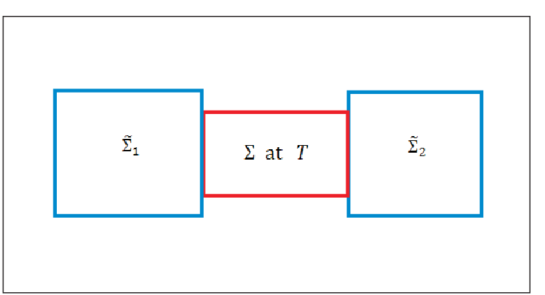
While most of the review deals with an isolated system or an interacting system in a medium, we will occasionally also consider a system interacting with two different media such as in Fig. 2, to study driven and steady macrostates Oono; Sasa; Bejan at for which there is no EQ macrostate having unique values of the temperature, pressure, etc. as long as we do not allow the media to come to EQ with each other, which takes much longer time . A steady or an unsteady macrostate always gives rise to irreversible entropy generation so it truly belongs to the realm of the NEQT. What makes the MNEQT a highly desirable approach is that it can also deal with unsteady processes easily as we will do.
I.1 Unique Macrostates in Extended State Space
The firm foundation of EQ statistical mechanics is accomplished by using the concept of microstates of and their EQ probabilities . This is feasible as the EQ macrostate is unique in the EQ state space spanned by the set of observables Note , where are the energy, volume, etc. using standard notation (we do not show the number of particles as we keep it fixed throughout this review Note0; see later, however). But the same cannot be said about its extension to describe NEQT, since NEQ macrostates in are not unique Kestin even if they appear in a process between two EQ macrostates, which we will always denote by and use for any general process including . It is clear that unless we can specify the microstates for uniquely, we cannot speak of their probabilities in a sensible way, but this is precisely what we need to establish a rigorous NEQ statistical mechanics of thermodynamic processes Keizer-Book; Schuss; Coffee; Jarzynski; Sekimoto; Seifert; Gujrati-LangevinEq; Stratonovich; Bochkov. The system is usually surrounded by an external medium , which we always take to be in EQ; see Fig. 1(b). The combination as the union forms an isolated system, which we assume to be stationary.
The lack of uniqueness of is handled in the MNEQT by using a well-established practice deGroot; Coleman; Maugin; Gujrati-II; Langer; Prigogine; Pokrovskii; Gujrati-Hierarchy by considering a properly extended state space spanned by , by including a set of internal variables, in which NEQ macrostates and microstates of interest can be uniquely specified during the entire process . Here, is internally generated within so it cannot be controlled by the observer Note. The use of internal variables in glasses, prime examples of NEQ systems, is well known, where they give rise to distinct relaxations of the glassy macrostate Davies; Gutzow; Nemilov; Langer; Goldstein. Their justification is based on the ideas of chemical reactions Prigogine0, and has been formalized recently by us Gujrati-Hierarchy to any NEQ macrostate . It is well known that internal variables contribute to irreversibility in , which justifies their important role in the NEQT. We give several examples for their need later in the review and a clear strategy to identify them for computation under different conditions. In , the unique ’s are specified by the collection of two independent quantities, which form a probability space . We can then pursue any followed by as the latter evolves in time to another (EQ or NEQ) unique macrostate. A major simplification occurs when this independence is maintained at each instant so that during the evolution, each microstate follows a trajectory (such as a Brownian trajectory) whose characteristics do not depend on as a function of time (Gujrati-LangevinEq, for example); the latter, of course, determines the trajectory probability . Thus, uniquely specifies in . For the same collection , different choices of describe different processes.
I.2 Layout
The review is divided into two distinct parts. The first part consisting of Sects. III-IX deals with the up-to-date foundation of the MNEQT for , regardless of whether it is isolated or interacting (in the presence of one or more a external sources). We have tried to make the new concepts and their physics as clear as possible so a reader can appreciate the foundation of the MNEQT, which can be complex at times. The most important one is that of the NEQ temperature as anticipated by Planck that is required to be defined globally over the system so that it can satisfy the Clausius statement about macroheat flow from hot to cold. The concepts of the generalized macroheat and the generalized macrowork are directly and uniquely defined in terms of SI-quantities that pertain to the system alone. Thus, they are capable of describing the irreversibilty in the system. A clear strategy to identify internal variables is discussed for carrying out thermodynamic computation. The other part consisting of Sects. X-XIV deals with various applications of the MNEQT, many of which cannot be studied within the M̊NEQT without imposing additional requirements. This part provides an abundant evidence of successful implementation of the MNEQT.
The layout of the paper is as follows. In the next section, we introduce our notation and give some useful definitions and new concepts without any explanation. This section is only for bookkeeping so that readers can come back to it to refresh the concepts in the manuscript later when they are not sure of their meanings. The next six sections deal with various new concepts and theory behind the MNEQT. Sect. III introduces the central concept of internal variables that are required for arbitrary NEQ macrostates . Many examples are given to highlight their importance for . They form the extended state space , which contains the state space as a proper subspace. The internal variables are irrelevant for EQ macrostates in . Sect. IV is also very important, where we introduce the concept of NEQ entropies based on the original ideas of Boltzmann. In this sense, the derivation of this entropy is thermodynamic in nature, and gives rise to an expression of that generalizes the Gibbs formulation of the entropy to NEQ macrostates. Using this formulation, we reformulate a previously given proof of the second law. In Sect. V, we formulate the statistical mechanics of the MNEQT, and discuss the statistical significance of and that provide a reformulation of the first law in terms of SI-quantities for any arbitrary process between any two arbitrary macrostates. The SI-quantities are determined by alone, even if it is interacting with its exterior, and its usage has neither been noted nor has been appreciated by other workers in the field. These generalized macroquantities are different from exchange macrowork and macroheat. In this reformulation, the first law includes the second law in that it contains all the information of the irreversibility encoded in . This formulation applies equally well to the exchange energy change and the internally generated energy change , which shows the usefulness of the formulation. In Sect. VI, which is the most important section for the foundation of the MNEQT, we discuss the conditions for to be uniquely specified in , and introduce the concept of the internal equilibrium (IEQ) to specify in . A parallel is drawn between and so that many results valid for also apply to , except that the latter has nonzero entropy generation (). The entropy of is a state function in , while that of a macrostate that lies outside of is not a state function. see later. The entropy of that lies outside is similarly not a state function of . We show that the NEQ entropy in Sect. IV reduces to the thermodynamic EQ entropy for and to the thermodynamic IEQ entropy for . We introduce the concept of a NEQ thermodynamic temperature as an inverse entropy derivative (). We show that this concept satisfies various sensible requirements (C1-C4) of a thermodynamic temperature, which is global over the entire system even if it is inhomogeneous. This, we believe, solves a long-standing problem of a NEQ temperature. In terms of , we show that the Clausius inequality in the M̊NEQT is turned into an equality in the MNEQT as shown in Sect. VII. In Sect. IX, which is the last section of the first part, we use the idea of chemical equilibrium to show how entropy is generated in an isolated system. We now turn to the second part of the review. In Sect. X, we consider various applications of the MNEQT ranging from a simple system to composite systems under various conditions. This section is very important in that we establish here that we can treat a system either (i) as a ”black box” of temperature but without knowing anything about its interior, or (ii) as a composite system for which we have a detailed information about its interior inhomogeneity. Both realizations give the same irreversible entropy generation. Thus, we can always treat a system as of temperature , whose study then becomes simpler. In Sect. XI, we apply our approach to a glassy system and derive the famous Tool-Narayanaswamy equation for the glassy temperature . In Sect. XII, we apply the MNEQT to study an irreversible Carnot cycle and determine its efficiency in terms of . In Sect. XIII, we apply the MNEQT to a very important problem of friction and the Brownian motion. In Sect. XIV, we consider a classical and a quantum expansion. In the classical case, we study the expansion in , where is a non-IEQ macrostate, with an explicit time-dependence, and in , where is a an IEQ macrostate, with no explicit time-dependence, and show that we obtain the same result. The quantum expansion is only studied in . The last section provides an extensive discussion of the MNEQT and draws some useful conclusions.
II Notation, Definitions and New Concepts
II.1 Notation
Before proceeding further, it is useful to introduce in this section our notation to describe various systems and their behavior and new concepts for their understanding without much or any explanation (that will be offered later in the review where we discuss them) so that a reader can always come back here to be reminded of their meaning in case of confusion. In this sense, this section plays an important role in the review for the purpose of bookkeeping.
Even though is macroscopic in size, it is extremely small compared to the medium ; see Fig. 1(b). The medium consists of two parts: a work source and a macroheat source , both of which can interact with the system directly but not with each other. This separation allows us to study macrowork and macroheat exchanges separately. We will continue to use to refer to both of them together. The collection forms an isolated system, which we assume to be stationary. The system in Fig. 1(a) is an isolated system, which we may not divide into a medium and a system. Each medium in Fig. 2, although not interacting with each other, has a similar relationship with , except that the collection forms an isolated system. In case they were mutually interacting, they can be treated as a single medium. In the following, we will mostly focus on Fig. 1 to introduce the notation, which can be easily extended to Fig. 2.
We will use the term ”body” to refer to any of , and in this review and use to denote it. However, to avoid notational complication, we will use the notation suitable for for if no confusion would arise in the context. As the mechanical aspect of a body is described by the Hamiltonian , whose value determines its macroenergy , it plays an important role in thermodynamics. Therefore, it is convenient to introduce
| (1) |
where means to delete from the set, and refers to the rest of the elements in besides . We use to denote the collection of coordinates and momenta of the particles in the phase space of . The variable appears as a parameter set in the Hamiltonian of that can be varied in a process with a concomitant change in . As internal variables play no role in EQ, in EQ. We will normally employ a discretization of the phase space in which we divide it into cells , centered at and of some small size, commonly taken to be . The cells cover the entire phase space. To account for the identical nature of the particles, the number of cells and the volume of the phase space is assumed to be divided by to give distinct arrangements of the particles in the cells, which are indexed by and write them as ; the center of is at . These cells represents the microstates . The energy and probability of these cells are denoted by in which is a function of . Different choices of for the same set describes different macrostates for a given , one of which corresponding to uniquely specifies an EQ macrostate ; all other states are called NEQ macrostates . Among are some special macrostates that are said to be in internal equilibrium (IEQ); the rest are nonIEQ macrostates . An arbitrary macrostate refers to either an EQ or a NEQ macrostate.
We use a suffix to denote all quantities pertaining to , a tilde for all quantities pertaining to , and no suffix for all quantities pertaining to even if it is isolated. Thus, the set of observables are denoted by and , respectively, and the set of state variables by and , respectively, in the state space ; the set of internal variables are and , respectively. As is taken to be in EQ, weakly interacting with and is extremely large compared to , all its fields can be safely taken to be the fields associated with so can be denoted by using the suffix .
In the discrete approach, and are spatially disjoint so
They are weakly interacting so that their energies are quasi-additive
where is the weak interaction energy between and and can be neglected to a good approximation. We also take them to be quasi-independent Gujrati-II so that their entropies also become quasiadditive:
| (2) |
here, is a negligible contribution to the entropy due to quasi-independence between and , and can also be neglected to a good approximation. The entropy has no explicit time dependence as is always assumed to be in equilibrium, and remains constant for the isolated system . The discussion of quasi-independence and its distinction from weak interaction has been carefully presented elsewhere (Gujrati-II, was called there; however, seems to be more appropriate) for the first time, which we summarize as follows. The concept of quasi-independence is determined by the thermodynamic concept of correlation length , which is a property of macrostates, and can be much larger than the interaction length between particles. A simple well-known example is of the correlation length of a nearest neighbor Ising model, which can be extremely large near a critical point than the nearest neighbor distance between the spins. This distinction is usually not made explicit in the literature. For quasi-independence between and , we require their sizes to be larger than . Throughout this review, we will think of the above approximate equalities as equalities to make the energies to be additive by neglecting the interaction energy between and , which is a standard practice in the field, but also assuming quasi-independence between them to make the entropies to be additive, which is not usually mentioned as a requirement in the literature.
For a reversible process, the entropy of each macrostate of a body along the process is a state function of , but not for an irreversible process for which . Their entropies are written as Gujrati-Entropy1; Gujrati-Entropy2 with an explicit time dependence. In general Gujrati-Symmetry; Landau; Gujrati-Entropy1; Gujrati-Entropy2,
| (3) |
The equilibrium values of various entropies are always denoted with no explicit time dependence such as by for . These entropies represent the maximum possible values of the entropies of a body as it relaxes and comes to equilibrium for a given set of observables. Once in equilibrium, the body will have no memory of its original macrostate. The set , which includes its energy among others, remains constant for as it relaxes Note. This notion is also extended to a body in internal equilibrium.
Notation 1
We use modern notation Prigogine; deGroot and its extension, see Fig. 1, that will be extremely useful to understand the usefulness of our novel approach. Any infinitesimal and extensive system-intrinsic quantity during an arbitrary process can be partitioned as
| (4) |
where is the change caused by exchange (e) with the medium and is its change due to internal or irreversible (i) processes going on within the system.
II.2 Some Definitions and New Concepts
Definition 2
Observables of a system are quantities that can be controlled from outside the system, and internal variables are quantities that cannot be controlled. Their collection is called the set of state variables in the state space .
Definition 3
A system-intrinsic quantity is a quantity that pertains to the system alone and can be used to characterize the system. A medium–intrinsic quantity is a quantity that is solely determined by the medium alone and can be used to characterize the exchange between the system and the medium.
Definition 4
A macrostate in or is a collection of microstates and their probabilities . In general, are functions of or , depending on the state space. They are implicit function of time through them; they may also depend explicitly on time if not unique in the state space.. For an EQ or an IEQ macrostate, have no explicit dependence on . For EQ states, have no time-dependence. It is through the microstate probabilities that thermodynamics gets its stochastic nature.
Definition 5
The collection provides a complete microscopic or statistical mechanical description of thermodynamics for in some state space in which one deals with macroscopic or ensemble averages, see Definition 13, over of microstate variables. The same collection also provides a microscopic description of a microstate and its probability in any arbitrary process.
Definition 6
The nonequilibrium macrostates can be classified into two classes:
- (a)
Internal-equilibrium macrostates (IEQ): The nonequilibrium entropy for such a macrostate is a state function in the larger nonequilibrium state space spanned by ; is a proper subspace of : . As there is no explicit time dependence, there is no memory of the initial macrostate in IEQ macrostates.
- (b)
Non-internal-equilibrium macrostates (NIEQ): The nonequilibrium entropy for such a macrostate is not a state function of the state variable . Accordingly, we denote it by with an explicit time dependence. The explicit time dependence gives rise to memory effects in these NEQ macrostates that lie outside the nonequilibrium state space . A NIEQ macrostate in becomes an IEQ macrostate in a larger state space , with a proper choice of .
Definition 7
An arbitrary macrostate (ARB) of a system refers to all possible thermodynamic states, which include EQ macrostates, and NEQ macrostates with and without the memory of the initial macrostate. We denote an arbitrary macrostate by , NEQ macrostates by , EQ macrostates by , and IEQ macrostates by .
Definition 8
Thermodynamic entropy is defined by the Gibbs fundamental relation for a macrostate.
Definition 9
Statistical entropy for is defined by its microstates by Gibbs formulation.
Definition 10
Changes in quantities such as in an infinitesimal processes are denoted by ; changes during a finite process are denoted by .
Definition 11
The path of a macrostate is the path it takes in during a process . The trajectory is the trajectory a microstate takes in time in during the process .
As evolves due to Hamilton’s equations of motion for given , the variation of has no effect on . Therefore, we will no longer exhibit and simply use for the Hamiltonian. The microenergy changes isentropically as changes without changing Gujrati-GeneralizedWork. Accordingly, the generalized macrowork does not generate any stochasticity. The latter is brought about by the generalized macroheat , which changes but without changing . In the MNEQT,
| (5a) | |||
| in terms of the temperature | |||
| (5b) | |||
| and of . The Eq. (5a) is a general result in the MNEQT. | |||
It is convenient to introduce as the set of all thermodynamic macrovariables, which takes the microvalue on .
Definition 12
This is an extension of the standard partition for the entropy change Prigogine; deGroot
| (7) |
For and , the partitions are
| (8) |
except that
| (9) |
for the simple reason that internal processes cannot change and , respectively. For , the partition is
with present when there is chemical reaction. We will find the shorthand notation
| (10) |
quite useful in the following for the various infinitesimal contributions. These linear operators satisfy
| (11) |
Definition 13
Ensemble Average: In NEQT, any thermodynamic macroquantity is obtained by the instantaneous ensemble average
| (12) |
where takes microvalues on at that instant with probability .
We have used the standard convention to write for . For example, the internal energy is given by
| (13) |
while the statistical entropy, often called the Gibbs entropy, is given by
| (14) |
where the microentropy is
| (15) |
in terms of Gibbs’ index of probability (Gibbs, p. 16).
Definition 14
Micropartition:The macropartition in Eq. (6a) is extended to microvariable :
| (16a) | |||
| Thus, | |||
| (16b) | |||
| The micropartition also applies to : | |||
| (17a) | |||
| We define | |||
| (17b) | |||
In a process, undergoes infinitesimal changes at fixed , or infinitesimal changes at fixed . The changes result in two distinct ensemble averages or process quantities.
Definition 15
Infinitesimal macroquantities are ensemble averages
| (18a) | |||
| at fixed so they are isentropic. We identify them as mechanical macroquantity and write it as . Infinitesimal macroquantities | |||
| (18b) | |||
| that are ensemble averages involving are identified as stochastic macroquantities and written as . Together, they determine the change : | |||
| (19) |
We must carefully distinguish and . For , we will use instead the following notation:
| (20) |
from which follows
| (21) |
Using Eq. (9) for , we have the following thermodynamic identity:
| (22) |
For , we have the following SI- and MI- formulation of the first law:
| (23a) | ||||
| (23b) | ||||
| where we have used the identity . The top equation is also known as the Gibbs fundamental relation. | ||||
We can use the operator identity in Eq. (11) to introduce the following important identities following Notation 1
| (24) | ||||
| (25) |
that will be very useful in the MNEQT. For an isolated system, . Note that , etc. do not represent changes in any SI-macrovariable.
Definition 16
We simply call and macroheat and macrowork, respectively, unless clarity is needed and use exchange macroheat for and exchange macrowork for , irreversible macroheat for and irreversible macrowork for , respectively.
Manipulating such as the ”volume” from the outside through requires some external ”force” , such as the external pressure to do some ”exchange macrowork” on . We have , and
| (26) |
where ; see Fig. 1. We use .
In a NEQ system, the generalized force in differs from . The resulting macrowork done by is
| (27) |
This is the SI-macrowork and differs from the MI-macrowork . Here,
| (28) |
see Fig. 1. The SI-affinity corresponding to Prigogine; Prigogine0 is nonzero, except in EQ, when it vanishes: deGroot; Prigogine. The ” SI-macrowork” done by as varies is
| (29) |
Even for an isolated NEQ system, will not vanish; it vanishes only in EQ, since does no work when ; however, and are unaffected by the presence of .
The macroforce imbalance is the difference
| (30a) | |||
| In general, controls the behavior of in Prigogine; Prigogine0 and vanishes when EQ is reached deGroot; Prigogine. Here, we will take a more general view of , and extend its definition to also. In particular, also plays the role of an affinity Gujrati-I so we can include it with to form set of thermodynamic macroforces or of macroforce imbalance: | |||
| (30b) | |||
| The same reasoning also shows that plays the role of an activity. | |||
The irreversible macrowork is given by
| (31) |
For the sake of clarity, we will take as a symbolic representation of , and a single as an internal variable in many examples. Then is the macrowork parameter. In this case, we have
| (32a) | ||||
| (32b) | ||||
| provided . | ||||
The microanalogue of is the internal microforce imbalance
| (33) |
which determines the internal microwork
| (34) |
as the exchange microwork is
| (35) |
III Internal Variables
We should emphasize that the concept of internal variables and their usefulness in NEQT has a long history. We refer the reader to an excellent exposition of this topic in the monograph by Maugin (Maugin, see Ch. 4). We consider a few simple examples to justify why internal variables are needed to uniquely specify a , and how to identify them for various systems.
It should be stated that in order to capture a NEQ process, internal variables are usually necessary. Another way to appreciate this fact is to realize that
Remark 17
For an isolated system, all the observables in are fixed so if the entropy is a function of only, it cannot change Gujrati-I; Gujrati-II; Gujrati-Entropy1; Gujrati-Entropy2 even if the system is out of EQ.
Thus, we need additional independent variables to ensure the law of increase of entropy for a NEQ isolated system. A point in represents , but a point represents . In EQ, internal variables are no longer independent of the observables. Consequently, their affinities (see later) vanish in EQ. It is common to define the internal variables so their EQ values vanish. We now discuss various scenarios where they are needed for a proper consideration.
III.1 A Two-level System
Consider a NEQ system of particles such as Ising spins, each of which can be in two levels, forming an isolated system of volume . Let and denote the probabilities and energies of the two levels of a particle in a NEQ macrostate so that keep changing. We have assumed that depends on the observable only, which happens to be constant for . We have for the average energy per particle, which is also a constant for , and
as a consequence of . Using , we get
which, for , is inconsistent with the first equation (unless , which corresponds to EQ). Thus, cannot be treated as constant in evaluating . In other words, there must be an extra dependence in so that
and the inconsistency is removed. This extra dependence must be due to independent internal variables that are not controlled from the outside (isolated system) so they continue to relax in as it approaches EQ. Let us imagine that there is a single internal variable so that we can express as in which continues to change as the system comes to equilibrium. The above equation then relates and ; they both vanish simultaneously as EQ is reached. We also see that without any , the isolated system cannot equilibrate; see Remark 17.
III.2 A Many-level System
The above discussion is easily extended to a with many energy levels of a particle with the same conclusion that at least a single internal variable is required to express for each level . We can also visualize the above system in terms of microstates. A microstate refers to a particular distribution of the particles in any of the levels with energy , where is the number of particles in the th level, and is obviously a function of so we will express it as ; we suppress the dependence on . This makes the average energy of the system also a function of , which we express as .
III.3 Disparate Degrees of freedom
In classical statistical mechanics, the kinetic and potential energies and , respectively, are functions of independent variables. Only their sum can be controlled from the outside, but not individually. Thus, one of them can be treated as an internal variable. In a NEQ macrostates, each term can have its own temperature. Only in EQ, do they have the same temperature.
This has an important consequence for glasses, where the vibrational degrees of freedom (dof) come to EQ with the heat bath at faster than the configurational degrees of freedom (dof), which have a different temperature than . The disparity in dof and dof cannot be controlled by the observer so it plays the role of an internal variable. A well-known equation, the Tool-Narayanaswamy equation is concerned with this disparity and is discussed in Sect. XI.
Consider a collection of semiflexible polymers in a solution on a lattice. The interaction energy consists of several additive terms as discussed in (Gujrati-II, Eq. (40)): the interaction energy between the polymer and the solvent, the interaction energy between the solvent, the interaction energy between polymers. Only the total can be controlled from the outside so the remaining terms determine several internal variables.
In the examples above, the internal variables are not due to spatial inhomogeneity. An EQ system is uniform. Thus, the presence of suggests some sort of nonuniformity in the system. To appreciate its physics, we consider a slightly different situation below as a possible example of nonuniformity.
III.4 Nonuniformity
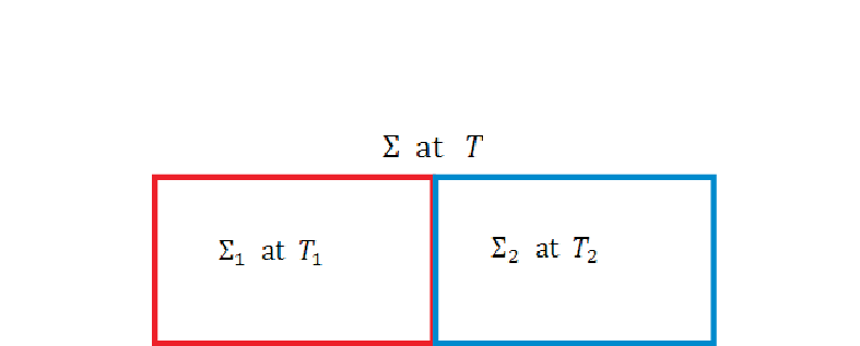
(a) We consider as a simple NEQ example a composite isolated system , see Fig. 3, consisting of two subsystems and of identical volumes and numbers of particles but at different temperatures and at any time before EQ is reached at so the subsystems have different time-dependent energies and , respectively. We assume a diathermal wall separating and . Treating each subsystem in EQ at each , we write their entropies as and , which we simply show as and as we will not let their volumes and particles numbers change. The entropy of is a function of and . Obviously, is in a NEQ macrostate at each . As and do not refer to , we form two independent combinations from and
| (36) |
that refer to so that we can express the entropy as for treated as a blackbox ; we do not need to know about its interior (its inhomogeneity) anymore. Here, plays the role of an internal variable, which continues to relax towards zero as approaches EQ. For given and , has the maximum possible values since both and have their maximum value. As we will see below, this is the idea behind the concept of internal equilibrium in which is a state function of state variables and continues to increase as decreases and vanishes in EQ. In this macrostate, has the maximum possible value for fixed so it becomes a state function; see Definition 30. This case and its various extensions are investigated in MNEQT in Sec. X.3.
(b) We can easily extend the model to include four identical subsystems of fixed and identical volumes and numbers of particles, but of different energies , and . Instead of using these independent variables, we can use the following four independent combinations
| (37) |
to express the entropy of as . The pattern of extension for this simple case of energy inhomogeneity. is evident.
(c) We make the model a bit more interesting by allowing the volumes and to also vary as equilibrates. Apart from the internal variable , we require another internal variable to form two independent combinations
| (38) |
so that we can use for the entropy of in terms of the entropies of and .
(d) In the above examples, we have assumed the subsystems to be in EQ. We now consider when the subsystems are in IEQ. We consider the simple case of two subsystems and of identical volumes and numbers of particles. Each subsystem is in different IEQ macrostates described by and . We now construct four independent combinations
| (39) |
which can be used to express the entropy of as .
(e) The example in (a) can be easily extended to the case of expansion and contraction by replacing , and by , and , see Fig. 6, to describe the diffusion of particles Vilar-Rubi. The role of and , etc. are played by and , etc.
III.5 Relative Motion in Piston-Gas System
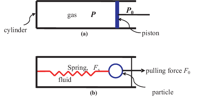
We now consider the motion of the piston in Fig. 4(a) because of the pressure difference across it. The discussion also shows how the Hamiltonian becomes dependent on internal variables, and how the system is maintained stationary despite motion of its parts.
Let denote the momentum of the piston. The gas, the cylinder and the piston constitute the system . We have a gas of mass in the cylindrical volume , the piston of mass , and the rigid cylinder (with its end opposite to the piston closed) of mass . However, we will consider the composite subsystem so that with it makes up . The Hamiltonian of the system is the sum of of the gas and cylinder, of the piston, the interaction Hamiltonian between the two subsystems and , and the interaction Hamiltonian between and . As is customary, see the discussion in Sect. II, we will neglect here. We assume that the centers-of-mass of and are moving with respect to the medium with linear momentum and , respectively. We do not allow any rotation for simplicity. We assume that
| (40) |
so that is at rest with respect to the medium. Thus,
| (41) |
where gc,p, denotes a point in the phase space of ; is the volume of , and is the volume of . We do not exhibit the number of particles as we keep them fixed. We let denotes the collection (). Thus, and the average energy depend on the parameters . As the relative motion cannot be controlled from the outside, one of the momenta plays the role of an internal variable.
III.6 Extended State Space
It should be clear from above that we can identify the entropy
If we divide into many subsystems so that they are all quasi-independent, then the entropy additivity gives
As we will be dealing with the Hamiltonian of the system, it is useful to introduce the notation in Eq. (1) with . Then, and become a function of as we will show in Sec. V. Here, appears as a parameter in the Hamiltonian, which we will write as , where is a point (collection of coordinates and momenta of the particles) in the phase space specified by . As an example, are the parameters in Sec. XIII. When the system moves about in the phase space , changes but as a parameter remains fixed in a state subspace ; see the discussion of Eq. (55a).
It is important to draw attention to the following important distinction between the Hamiltonian and the ensemble average energy ; see Eq. (44). While accounts for the stochasticity through microstate probabilities, the use of the Hamiltonian is going to be restricted to a particular microstate. In other words, the Hamiltonian depends on and but the energy depends on the entropy and . The energy of , on the other hand, depends only on and denotes the value of for . In the following, we will always treat Hamiltonians and microstate energies as equivalent description, which does not depend on knowing ; the average energies depend on for their definition; see Eq. (13).
IV NEQ Entropy
IV.1 Determination of
The uniqueness issue about the NEQ macrostate says nothing about the entropy of an arbitrary (so it may be nonunique) macrostate , which is always given by the Gibbs entropy in Eq. (14); see also Shannon. The ensemble averaging implies that the entropy is a statistical concept, as is the energy , Eq. (13).
We now justify the Gibbs’ statistical formulation of for any arbitrary in thermodynamics. The demonstration follows a very simple combinatorial argument Gujrati-Entropy2 using Boltzmann concept of thermodynamic entropy. In the demonstration, is not required to be uniquely identified. This entropy satisfies the law of increase of entropy as is easily seen by the discussion by Landau and Lifshitz Landau for a NEQ ideal gas Note-Landau in to derive the equilibrium distribution. Thus, the form in Eq. (14) is not restricted to only uniquely identified ’s. Hopefully, this will become clear below.
Proposition 18
The Second Law The NEQ Gibbs entropy of an isolated system is bounded above by its equilibrium entropy and continuously increases towards it so that Landau
| (42) |
IV.2 General Formulation of the Statistical Entropy
We focus on a macrostate of some body at a given instant , which refers to the set of microstates and their probabilities . The microstates are specified by , and may not uniquely specify the macrostate . Thus, even the set need not be uniquely specified. In the following, we will use the set for the set for simplicity. We will also denote by so that we can separate out the explicit variation due to . For simplicity, we suppress in in the following. For the computation of combinatorics, the probabilities are handled in the following abstract way. We consider a large number of independent replicas or samples of , with some large integer constant and the number of distinct microstates . We will see that is determined by ’s having nonzero probabilities. We will call them available microstates. The samples should be thought of as identically prepared experimental samples Gujrati-Symmetry.
Let denote the sample space spanned by , and let denote the number of th samples (samples specified by ) so that
| (43) |
The above sample space is a generalization of the ensemble introduced by Gibbs, except that the latter is restricted to an equilibrium body, whereas refers to the body in any arbitrary macrostate so that may be time-dependent, and need not be unique. The ensemble average of some quantity over these samples is given by Eq. (12). Thus,
| (44) |
where is the value of in .
The samples are, by definition, independent of each other so that there are no correlations among them. Because of this, we can treat the samples to be the outcomes of some random variable, the macrostate . This independence property of the outcomes is crucial in the following. They may be equiprobable but not necessarily. The number of ways to arrange the samples into distinct microstates is
| (45) |
Taking its natural log, as proposed by Boltzmann, to obtain an additive quantity per sample as
| (46) |
and using Stirling’s approximation, we see easily that it can be written as the average of the negative of Gibbs’ index of probability:
| (47) |
where we have also shown an explicit time-dependence, which merely reflects the fact that it is not a state function in , a reflection of the fact that is not uniquely specified in . We have put back above for clarity. Thus, Eq. (47) is nothing but Eq. (14) in form, and thus justifies it for an arbitrary .
The above derivation is based on fundamental principles and does not require the body to be in equilibrium; therefore, it is always applicable for any arbitrary macrostate . To the best of our knowledge, even though such an expression has been extensively used in the literature for NEQ entropy, it has been used by simply appealing to the information entropy Shannon.
The distinction between the Gibbs’ statistical entropy and the thermodynamic entropy should be emphasized. The latter appears in the Gibbs fundamental relation that relates the energy change with the entropy change as is well known in classical thermodynamics, and as we will also demonstrate below; see also Eq. (23a). The concept of microstates is irrelevant for this, which is a purely thermodynamic relation. On the other hand, is solely determined by so its a statistical quantity. It then becomes imperative to show their equivalence, mainly because is based on the Boltzmann idea. This equivalence has been justified elsewhere Gujrati-Entropy1; Gujrati-Entropy2, and will be briefly summarized below.
Remark 19
Because of this equivalence, we will no longer make any distinction between the statistical Gibbs entropy and the thermodynamic entropy and will use the standard notation for both of them.
Remark 20
The Gibbs entropy appears as an instantaneous ensemble average, see Definition 13. This average should be contrasted with a temporal average in which a macroquantity is considered as the average over a long period of time
where is the value of at time Landau. For an EQ macrostate , both definitions give the same result provided ergodicity holds. The physics of this average is that at represents a microstate of . As is invariant in time, these microstates belong to , and the time average is the same as the ensemble average if ergodicity holds. However, for a NEQ macrostate , which continuously changes with time, the temporal average is not physically meaningful as the microstate at time corresponds to and not to in that the probabilities and are different in the two macrostates. Only the ensemble average makes any sense at any time as was first pointed out in Gujrati-ResidualEntropy. Because of this, we only consider ensemble averages in this review.
The maximum possible value of for given occurs when are uniquely specified in . This makes a state function of with no explicit time dependence, which we write as . Thus,
| (48) |
The simplest way to understand the physical meaning is as follows: Consider at some time . As may not be a unique function of , we look at all possible entropy functions for this . These entropies correspond to all possible sets of for a fixed , and define different possible macrostates . We pick that particular among these that has the maximum possible value of the entropy, which we denote by or without any explicit -dependence. This entropy is a state function . For a macroscopic system, this occurs when the corresponding microstate probabilities for are
| (49a) | |||
| so that | |||
| (49b) | |||
| We wish to point out the presence of nonzero probabilities in Eq. (49a) that explains the comment above of available microstates. Including microstates with zero probabilities will not correcting account for the number of microstates with given . | |||
There is an alternative to the above picture in which we can imagine the for which has been fixed, which essentially ”isolates” and converts it into a . Then, as varies, its entropy increases until it reaches its maximum value in accordance with Proposition 18.
Remark 21
We emphasize that so above in Eq. (49a) is determined by the average energy and not by the microstate energy as derived later in Sect. (VIII.2). The in Eq. (49a) basically replaces the actual probability distribution in Eq. (101) by a flat distribution of height and width , a common practice in the thermodynamic limit of statistical mechanics Landau. Despite this modification, the entropy has the same value for a macroscopic system, for which and are given by Eqs. (72) and (73), respectively; see also Sect. VIII.2.
Let us consider a different formulation of the entropy for a macrostate specified by some at some instance . This macrostate provides a more incomplete specification than in . Applying the above formulation to , and consisting of microstates forming the set with probabilities , we find that
| (50) |
is the entropy of ; here is the number of distinct microstates . It should be obvious that
Again, under the equiprobable assumption
denoting the sample space spanned by , the above entropy takes its maximum possible value
| (51) |
which is the well-known value of the Boltzmann entropy for a body in equilibrium
| (52) |
and provides a statistical definition of, and hence connects it with the, thermodynamic entropy of the body proposed by Boltzmann. The maximization again has the same implication as in Eq. (48): For given , we look for the maximum entropy at all possible times. It is evident that
| (53) |
Thus, the NEQ entropy as , the equilibration time, reduces to in EQ, as expected. Before equilibration, in remains a nonstate function in where we do not invoke . It is the variation in that is responsible for the time variation in . A simple proof of this conclusion is given in Sect. VIII.3; see Remark 49 also. We can summarize this conclusion as
Conclusion 22
The variation in time in in is due to the missing set of internal variables .
We now revert back to the standard use of , and . Let us consider a body , which we take to be isolated and out of equilibrium so that its macrostate spontaneously relaxes towards at fixed . Its entropy in has an explicit time dependence, which continue to increase towards . For such NEQ states, the explicit time dependence in is explained by introducing to make their entropies a state function in an appropriately chosen larger state space Gujrati-II. It is also shown there that a NIEQ macrostate with a nonstate function entropy may be converted to an IEQ macrostate with a state function entropy by going to an appropriately chosen larger state space spanned by with its proper subspace. Therefore, in most cases of interest here, we would be dealing with a state function and usually write it as , unless a choice for has been made based on the experimental setup. In that case, we must deal with a pre-determined state space so that some NEQ states that lie outside can become a state function in some .
We have discussed above that the explicit time dependence in a NEQ macrostate with a nonstate function entropy is due to additional state variables in and that this NEQ macrostate may be converted into an IEQ macrostate with a macrostate function entropy by going from to an appropriately chosen larger state space . Similarly, it has been shown Gujrati-II that a NIEQ macrostate in with a nonstate function entropy may be converted to an IEQ macrostate in an appropriately chosen larger state space with a state function entropy .The additional internal variables that are over and above in give rise to additional entropy generation as they relax for fixed . This results in the following inequality:
| (54) |
However, if the choice for has been made based on the experimental setup and the observation time , see Sect. VIII.1, we must restrict our discussion to so that we must consider in the following. This will be done in Sect. VIII.3; see Remarks 46 and 49.
IV.3 A Proof of The Second Law
The second law has been proven so far under different assumptions (Tolman; Rice; Jaynes; Gujrati-ResidualEntropy; Gujrati-Symmetry, among others). Here, we provide a simple proof of it based on the postulate of the flat distribution; see Remark 21. The current proof is an extension of the proof given earlier see also (Gujrati-Symmetry, Theorem 4). We consider an isolated system for which the second law is expressed by Eq. (42). However, for simplicity, we will suppress the subscript from all the quantities in this section. As the law requires considering the instantaneous entropy as a function of time, we need to focus on the sample space at each instant to determine its entropy as a function of time. At each instance, it is an ensemble average over the instantaneous sample space formed by the instantaneous set of available microstates, see Eq. (14) or (47). We will use the flat distributions for the microstates at each instance, see Remark 21, so that the entropy is given by Eq. (49b).
To prove the second law, see Proposition 18, we proceed in steps by considering a sequence of sample spaces belonging to as follows Gujrati-ResidualEntropy; Gujrati-Symmetry. At a given instant, a system happens to be in some microstate. We start at , at which time happens to be in a microstate, which we label . It forms a sample space containing with probability , with the superscript denoting the sample space. We have . At some , the sample space is enlarged from to , which contains and , with probabilities and . Using the flat distribution, the entropy is now . We just follow the system in a sequence of time so that at , we have a sample space with so that . Continuing this until all microstates in have appeared, we have .
Thus, we have proven that the entropy continues to increase until it reaches its maximum in accordance with Proposition 18.
V Hamiltonian Trajectories in
V.1 Generalized Microforce and Microwork for
Traditional formulation of statistical thermodynamics Landau; Gibbs; Gujrati-Symmetry takes a mechanical approach in which follows its classical or quantum mechanical evolution dictated by its SI-Hamiltonian . The quantum microstates are specified by a set of good quantum numbers, which we have denoted by above as a single quantum number for simplicity; we take denoting the set of natural numbers. We will see below that does not change as changes. In the classical case, we use a small cell around as discussed above as the microstate . The Hamiltonian gives rise to a purely mechanical evolution of individual ’s, which we will call the Hamiltonian evolution, and suffices to provide their mechanical description. The change in in a process is
| (55a) | |||
| The first term on the right vanishes identically due to Hamilton’s equations of motion for any . Thus, for fixed , the energy remains constant as moves about in . Only the variation in generates any change in . Consequently, we do not worry about how changes in in the phase space, and focus, instead, on the state space , in which can write | |||
| (55b) | |||
| where denotes the generalized microwork produced by the generalized microforce : | |||
| (55c) | |||
| For the case , the corresponding microforce is (, where | |||
| (56) |
The corresponding microwork is
| (57) |
V.2 Statistical Significance of and
Before proceeding further, let us see how the generalized macrowork and macroheat could be understood from a statistical point of view so that we can identify them using the Hamiltonian. Once has been identified, the Hamiltonian must be expressed in terms of it. Thus, and are functions of in . We now prove
Theorem 23
is a function of and for any , even though ’s are functions of only.
Proof. We consider the differential
| (58) |
As ’s are unchanged in the first sum, this sum is evaluated at constant entropy so this is purely mechanical macroquantity ; see Eq. (20). This sum is a function of as is seen clearly in Eq. (55b). The second contribution is at fixed microstate energies so is held fixed, but require changes in the probabilities so it is the stochastic contribution , see Eq. (55b). The changes result in is . As and
| (59) |
are both extensive, they must be linearly related with an intensive constant of proportionality. This proves that is a function of and in general for any .
Note that we have used the identity above; see also Eq. (108).
We introduce a special process, to be called a generalized isometric process, which is a process at fixed and is a generalization of an isochoric process. In this process, the work done by each mechanical variables in remains zero so . We now prove the following theorem that establishes the physical significance of the two contributions.
Theorem 24
The isentropic contribution represents the generalized macrowork and the stochastic contribution represents the generalized macroheat for any .
Proof. We follow Landau and Lifshitz Landau and rewrite the first term in Eq. (58) as
where we have used Eq. (55c). The use of Eqs. (64a) and (64b) proves that
| (60) |
is the isentropic contribution, making macrowork a mechanical concept as we have already pointed out. This identification then also proves that the macroheat in the first law, see Eq. (23a), must be properly identified with . Accordingly,
| (61) |
is purely stochastic.
The linear proportionality between and mentioned above in the proof of Theorem 23 results in
| (62) |
which is a statistical proof of the identity in Eq. (5a) relating and for any . We also note that the ratio is related to the ratio of two SI-macroquantities. Thus, it can be used to characterize the instantaneous macrostate . This should be contrasted with the M̊NEQT, in which the ratio
| (63) |
does not characterize the instantaneous macrostate . In Eq. (104), we provide a general procedure for a thermodynamic identification of .
Remark 25
It is worth emphasizing that and in Eqs. (61-59) are defined as instantaneous quantities in terms of the instantaneous changes , regardless of the speed of the segmental process , and instantaneous values and . Therefore, the generalized macroheat and entropy change are defined regardless of the speed of the arbitrary process. As in Eq. (58) is also defined instantaneously, it is clear from Eq. (23a) that the generalized work is also defined instantaneously regardless of the speed of the arbitrary process. This is consistent with our above derivation of in terms of generalized forces. The observation is very important as it shows that the existence of all SI-quantities does not depend on the speed of the arbitrary process . However, see also Sect. VIII.1 further clarification on the importance of . From now onward, we will not make a distinction between and .
We should point out that, as is a parameter, is the same for all microstates. The statistical nature of is reflected in the statistical nature of , such as and , of the system. Thus, the SI-fields are fluctuating quantities from microstate to microstate as expected in any averaging process.
We can now identify as the macrowork parameter, and the variation in defines not only the microwork , but also a thermodynamic process . The trajectory in followed by as a function of time will be called the Hamiltonian trajectory during which varies from its initial (in) value to its final (fin) value during , the the path denotes the path the macrostate follows during this process; see Definition 11. The variation produces the generalized microwork . As plays no role in , its determination is simplifies in the MNEQT. The microwork also does not change the index of as said above. The ensemble average of is , see Eq. (28),
| (64a) | |||
| that of is given by | |||
| (64b) | |||
| as given earlier in Eq. (27). It is based on using the mechanical definition (force X displacement) of work. The macroforce corresponding to is , where , and . The corresponding SI-macrowork is given earlier in Eq. (32a). | |||
The above discussion proves that the definition of macroheat and macrowork is valid for any . It is useful to compare the above approach with the traditional formulation of the first law in terms of and : both formulations are valid in all cases. It should be mentioned that the above identification is well known in equilibrium statistical mechanics, but its extension to irreversible processes and our interpretation is, to the best of our knowledge, novel. While the instantaneous average such as the pressure is mechanically defined under all circumstances, it will only be identified with the thermodynamic definition of the instantaneous pressure
| (65) |
for a uniquely identified macrostate in .
Being purely mechanical in nature, a trajectory is completely deterministic and cannot describe the evolution of a macrostate during unless supplemented by thermodynamic stochasticity, which requires as discussed above Landau. Thermodynamics emerges when quantities pertaining to the trajectories are averaged over the trajectory ensemble with appropriate probabilities that will usually change during the process.
Conclusion 26
The change consists of two independent contributions- an isentropic change , and an stochastic change . On the other hand, the MI-macroheat and the MI-macrowork suffer from ambiguity; see, for example, Kestin Kestin.
Remark 27
It is clear from the above discussion that it is the macroheat and not the macrowork that causes , and therefore the entropy to change. This is the essence of the common wisdom that heat is random motion. But we now have a mathematical definition: macroheat is the isometric part of that is directly related to the change in the entropy through changes in . Macrowork is that part of the energy change caused by isentropic variations in the ”mechanical” state variables . This is true no matter how far the system is from equilibrium. Thus, our formulation of the first law and the identification of the two terms is the most general one, and applicable to any .
Remark 28
The relationship between the macroheat and the entropy becomes simple only when happens to be in internal equilibrium, see Sec. VI.1, in which case is replaced by , which has a thermodynamic significance; see Eq. (72) and we have the thermodynamic identity, called the Clausius Equality in Eq. (5a) for , which is very interesting in that it turns the well-known Clausius inequality into an equality.
For the sake of completeness, we briefly discuss the various attempts to the study of the microanalogs and of the and , respectively, that has flourished into an active field in diverse branches of NEQT at diverse length scales from mesoscopic to macroscopic lengths Bochkov; Jarzynski; Crooks; Pitaevskii; Sekimoto; Sekimoto-Book; Seifert; Lebowitz; Alicki; see also some recent reviews Seifert-Rev; Maruyama; Broeck. Unfortunately, this endeavor is apparently far from complete Gislason; Bertrand; Bauman; Kestin; Kievelson; Bizarro; Honig; Jarzynski; Rubi; Peliti; Cohen; Sekimoto; Seifert; Nieuwenhuizen; Crooks; Jarzynski-Cohen; Sung; Gross; Jarzynski-Gross; Jarzynski-Rubi; Rubi-Jarzynski; Peliti-Rubi; Rubi-Peliti; Pitaevskii; Bochkov; Maruyama; Seifert-Rev; Broeck; Sekimoto-Book; Lebowitz; Alicki. This is because of the confusion about the meaning of macrowork and macroheat even in classical NEQT Fermi; Kestin involving SI- or MI- description, which has only recently been clarified Gujrati-Heat-Work0; Gujrati-Heat-Work; Gujrati-I; Gujrati-II; Gujrati-III; Gujrati-Entropy1; Gujrati-Entropy2; Gujrati-LangevinEq in the MNEQT, where a clear distinction is made between the generalized macrowork (macroheat) () and the exchange macrowork (macroheat) (). In an EQ process, both macroworks (macroheats) have the same magnitude, but not in a NEQ process, where the difference determines ().
It is important to draw attention to the following important fact. We first recognize that the first law in Eq. (23b) refers to the change in the energy caused by exchange quantities. Therefore, on the left truly represents . Accordingly, we write Eq. (23b) as
| (66) |
which justifies Eq. (21) for . Subtracting this equation from Eq. (23a), we obtain the identity
| (67) |
which not only justifies Eq. (21) for but also Eq. (22) for which we have used Eq. (9).
Remark 29
The above analysis demonstrates the important fact that the first law can be applied either to the exchange process () or to the interior process (). The last formulation is also applicable to an isolated system.
V.3 Medium
The above discussion can be easily extended to the medium (the suffix denotes its microstates) with the following results
| (68) | ||||
where all the quantities including refer to the medium, except and , and have their standard meaning. The analog of Eq. (62) is as expected; see Eq. (63). We clearly see that
| (69a) | |||
| such as when mechanical equilibrium is not present. In this case, we also have | |||
| (69b) | |||
| with in view of Eq. (22). In a finite process , all infinitesimal quantities are replaced by their net changes | |||
| (69c) | |||
| where is obtained by integrating in Eq. (77c) over ; the result is given in Eq. (82), where it is discussed. | |||
V.4 Irreversible Macrowork and Macroheat
VI Unique Macrostates
VI.1 Internal Equilibrium
We now revert back to the original notation and . We will refer to in terms of microstate number in Eq. (49b) as the time-dependent Boltzmann formulation of the entropy or simply the Boltzmann entropy Lebowitz, whereas in Eq. (51) represents the equilibrium (Boltzmann) entropy. It is evident that the Gibbs formulation in Eqs. (47) and (50) supersedes the Boltzmann formulation in Eqs.(48) and (51), respectively, as the former contains the latter as a special limit. However, it should be also noted that there are competing views on which entropy is more general Lebowitz; Ruelle. We believe that the above derivation, being general, makes the Gibbs formulation more fundamental. The continuity of follows directly from the continuity of . Its existence follows from the observation that it is bounded above by and bounded below by , see Eq. (49b).
We now introduce the central concept of the MNEQT, which is based on the existence of above; see Definition 6, which we now expand.
Definition 30
A NEQ macrostate whose entropy is a state function in is said to be an internal equilibrium (IEQ) macrostate Gujrati-I; Gujrati-II; if not, its entropy is an explicit function of time in . An IEQ-macrostate in is a unique macrostate in .
We clarify this point. If we do not use for , which is not unique in , then its entropy cannot be a state function in , and must be expressed as . Thus, the importance of is to be able to deal with a state function entropy by choosing an appropriate number of internal variables. Throughout this work, we will only deal with IEQ macrostates. However, as we will see, our discussion of NEQ macrowork will cover all states.
Being a state function, shares many of the properties of EQ entropy , see Definition 6:
- 1.
Maximum: is the maximum possible value of the NEQ entropy in for a given Gujrati-II.
- 2.
No memory -Its value also does not depend on how the system arrives in , i.e., whether it arrives there from another IEQ macrostate or a non-IEQ macrostate Gujrati-II. Thus, it has no memory of the earlier macrostate.
There are some macrostates that emerge in fast changing processes such as the free expansion that possess memory of the initial states so that their entropy will no longer be a state function in . In this case, we need to enlarge the state space to by including internal variables as done in Sec. XIV.
Remark 31
It may appear to a reader that the concept of entropy being a state function is very restrictive. This is not the case as this concept, although not recognized by several workers, is implicit in the literature where the relationship of the thermodynamic entropy with state variables is investigated. To appreciate this, we observe that the entropy of a body in internal equilibrium Gujrati-I; Gujrati-II is given by the Boltzmann formula in Eq. (49b) in terms of the number of microstates corresponding to . In classical nonequilibrium thermodynamics deGroot, the entropy is always taken to be a state function. In the Edwards approach Edwards for granular materials, all microstates are equally probable as is required for the above Boltzmann formula. Bouchbinder and Langer Langer assume that the nonequilibrium entropy is given by Eq. (49b). Lebowitz Lebowitz also takes the above formulation for his definition of the nonequilibrium entropy. As a matter of fact, we are not aware of any work dealing with entropy computation that does not assume the nonequilibrium entropy to be a state function. This does not, of course, mean that all states of a system are internal equilibrium states. For states that are not in internal equilibrium, the entropy is not a state function so that it will have an explicit time dependence. But, as shown elsewhere,Gujrati-II this can be avoided by enlarging the space of internal variables. The choice of how many internal variables are needed will depend on experimental time scales and cannot be answered in generality just as is the case in EQ thermodynamics for the number of observables; the latter depends on the experimental setup. A detailed discussion is offered elsewhere Gujrati-Hierarchy.
VI.2 Gibbs Fundamental Relation
Being a state function, in for results in the following Gibbs fundamental relation for the entropy
| (71a) |
which can be inverted to express the Gibbs fundamental relation for the energy as
| (71b) |
where we have introduced
| (72) | ||||
| (73) |
as the inverse temperature of the system (we set the Boltzmann constant throughout the review), and have used Eq. (28) for the generalized macroforce . Recalling Eq. (64b), we see that the second term in Eq. (71b) is nothing but the SI-macrowork . Comparing Eq. (71b) with Eq. (23a), we can identify the generalized macroheat with , which then proves Eq. (5a).
It should be stated here that the choice and the number of state variables included in or is not so trivial and must be determined by the nature of the experiments Maugin. We will simply assume here that they have been specified. Just as is a state function of for in , there are in for which is a state function of .
The possibility of a Gibbs fundamental relation for is deferred to Sect. VIII.3.
VI.3 A Digression on the NEQ-Temperature
While the concept of the macrowork is quite familiar from mechanics, the concept of the macroheat is peculiar to thermodynamics in view of Eq. (5a). In EQ thermodynamics, the macroheat is directly proportional to the change , and the constant of proportionality determines the EQ temperature . Indeed, the concepts of entropy and of temperature are unique to thermodynamics and are well established in EQ thermodynamics. A in thermal equilibrium with a at obviously has the same temperature . The temperature for an isolated system in equilibrium is also well defined; its inverse is identified with the energy derivative of the equilibrium entropy Landau. The definition is valid for all EQ systems, even those containing gravitational interaction. This is confirmed by the fact that Bekenstein used it to identify the temperature of an isolated black hole Bekenstein; Hawking. The formulation is valid both classically and quantum mechanically Landau.
The EQ definition of the temperature is formally identical to that in Eq. (72), which is valid in NEQT Gujrati-Symmetry; Gujrati-Heat-Work0; Gujrati-Heat-Work; Gujrati-Entropy1; Gujrati-Entropy2; Gujrati-I; Gujrati-II; Gujrati-III. In this, we have a general thermodynamic definition of a temperature for any . It is important to realize that the notion of a NEQ temperature is an absolute necessity for the Clausius statement of the second law that the exchanged macroheat flows spontaneously from hot to cold to be meaningful.
It is clear from the above discussion that macrowork is the isentropic change in the energy, while macroheat is the energy change due to the entropy change. This is not as surprising a statement as it appears, since a mechanical system is usually thought of as a system for which the entropy concept is not meaningful. A different way to state this is that the entropy remains constant (isentropic) in any mechanical process as we have done above. Planck Planck had already suggested that the temperature should be defined for NEQ macrostates just as the entropy should be defined for them if we need to carry out a thermodynamic investigation of a NEQ system. Such a temperature was apparently first introduced by Landau Landau0 for partial set of the degrees of freedom (dof). This then allows the possibility that the notion of temperature can be separately applied, for example, to vibrational and configurational dof in glasses that are known to be out of equilibrium with each other Goldstein in that they are ascribed different temperatures. This means that macroheat would be exchanged between them until they come to equilibrium, but this is internally exchanged. But there seems to be a lot of confusion about the meaning of the entropy and temperature in NEQT (Muschik; Keizer; Morriss; Jou; Hoover; Ruelle; Evans; Oono; Maugin, for example), where different definitions lead to different results. In contrast, the meaning of entropy and fields in equilibrium thermodynamics has no such problem.
We agree with Planck and believe that there must exist a unifying approach to identify the temperature for ; see Definition 7, with or without memory effects in . The inverse temperature defined above in Eq. (72) is not directly applicable to nonIEQ-macrostates in for which is not a state function, but can be extended to them so as to accommodate memory effects as we do in Sect. VIII.3. However, we will not consider them in detail in this review.
Criterion 32
The identification of temperature in must satisfy some stringent but obvious criteria:
- C1
It must be intensive and must reduce to the temperature determined by Eq. (72) for and even for an isolated system.
- C2
It must cover negative temperatures Ramsey that are commonly observed for some dof such as nuclear spins in a system. As these dof are not involved in any macroscopic motion (Landau, Sec. 73), there is no kinetic energy involved. Most common occurrence of a negative temperature is when the above spin dof are out of equilibrium with the other dof such as lattice vibrations in the system.
- C3
It must satisfy the Clausius statement that macroheat between two objects always flows spontaneously from hot to cold for positive temperatures. When negative temperatures are considered, macroheat must flow from a system at a negative temperature to a system at a positive temperature.
- C4
It must be a global rather than a local property of the system so that we can differentiate hot and cold between two different systems.
The first criterion ensures that the new temperature is an extension of the conventional notion of the temperature that is valid when the entropy is a state function. This means that the new notion of temperature is valid for any arbitrary macrostate. In addition, it must exist even for an isolated system. The second criterion ensures that our formalism includes negative temperatures that may occur in a lattice system. The third criterion ensures compliance with the second law for interacting systems. This is a very important criterion, which every notion of temperature must satisfy. We will come back to this issue again in Sec. VI.5 where we prove it in the MNEQT. The last criterion ensures that the temperature is associated with the entire system, whether the system is homogeneous or not. This will be explained by direct calculations of inhomogeneous systems in Sect. X. By extension, the concept of a NEQ temperature can be also applied to different dof of a system such as a glass under the assumption that they are weakly interacting in accordance with the approach taken by Landau Landau0. This results in the Tool-Narayanaswamy relation derived in Sect. XI.
Before we close this discussion, we wish to point out major differences between the NEQ temperature in the MNEQT and its other definitions. We first consider the M̊NEQT. The most important theories belonging to this class are the classical local irreversible thermodynamics (LNEQT) deGroot, the rational thermodynamics (RNEQT) ColemanRational, and the extended irreversible thermodynamics (ENEQT) Jou as we had mentioned earlier. We refer the reader to Maugin; Jou for excellent reviews on these theories that use local densities of energy and entropy . They are continuum theories, and can all be classified as continuum M̊NEQT to be denoted by the CNEQT here. We consider them critically later in Sect. XV. They differ in the choice of their state spaces. Considering the local entropy and energy densities and , the inverse local temperature is defined as , and differs from the global temperature in the MNEQT.
- 1.
In the LNEQT, each local volume element is in EQ so the local temperature is the EQ temperature of the volume element, and differs from , which is a global temperature.
- 2.
In the RNEQT, the temperature is taken as a primitive quantity along with the entropy. Because of the memory effect, the temperature at any time depends on the entire history. Thus, it is a local analog of the global temperature of in the MNEQT, but the latter is defined thermodynamically.
- 3.
In the ENEQT, the fluxes are part of the state variables so the local temperature also depends on them. Assuming the total entropy to also depend on the fluxes (Jou0, see Eq. (5.66), for example), one can identify the global analog of the temperature in the ENEQT. However, as fluxes are MI-quantities, this temperature cannot be compared with the SI-temperature in the MNEQT.
There is a recent attempt Lucia to introduce another NEQ temperature by using fluctuation theorems to determine the entropy generation, which is then related to the Gouy-Stodola theorem derived later (see Eq. (84b)). It is limited to a interacting in a medium so does not apply to an isolated system. In addition, its validity is limited to the situation when the Gouy-Stodola theorem is valid as seen from the derivation of Eq. (84b).
VI.4 Uniqueness of and
We now give an alternative demonstration of the uniqueness of the entropy of in , which is based on the discussion of the internal variables in Sect. III. Let us assume that we divide into a finite number of nonoverlapping EQ subsystems such that . Without loss of generality, we assume that the subsystems are not in EQ with each other (their fields are not identical) so that is in a NEQ macrostate. Let denote the correlation length of , and we define to denote the maximum correlation length determining quasi-independence required for entropy additivity as discussed in Sect. II; see Eq. (2). For this, we need to take the linear size of . The EQ microstate of is uniquely described in . The additivity of entropy gives that must be a function of . Moreover, since each has a unique entropy , also has a unique value
| (74a) | |||
| As we need to express in terms of , we need additional independent linear combinations made from the set as already discussed in Sect. III to ensure that depends on the same number of state variables as there are in . This uniquely defines | |||
| (74b) | |||
| in in terms of the unique values. It is a mathematical identity between the left side for and the right side for . We can also take ’s to be in ’s in ’s so that are also uniquely defined. Then, the same reasoning as above also proves that | |||
| (74c) | |||
| is unique by ensuring that the number of arguments are the same on both sides between the entropies for and . | |||
We now prove the following central theorem on the existence of NEQ entropy for any with independent state variables.
Theorem 33
Existence: The SI-entropy for any exists, has a unique thermodynamic temperature , and is additive in .
Proof. According to the postulates of classical thermodynamics, EQ entropies exist in and are continuous. Therefore, Eq. (74a) proves the existence of the entropy for any in the state space , and is continuous. It follows from the existence of that has a unique thermodynamic temperature . In addition, is also additive as follows from Eq. (74c). This proves the theorem.
Corollary 34
The state space contains as a proper subspace because of the presence of the internal variables, except when is in EQ, when they become the same.
Proof. For any , contains all possible linear combinations of made from the set . Hence, it contains as a proper subspace. In EQ, internal variables become superfluous as they are no longer independent so their affinity vanishes. Thus, reduces to in EQ.
VI.5 Irreversibility Inequalities in
We consider the Hamiltonian in . We only consider the case of extensive macrowork parameters. As evolves under the variation in , its energy changes by without changing ; see Eq. (55b). The change determines the isentropic generalized macrowork . The stochasticity appears from the generalized macroheat . Recalling that for , , we have in general,
| (75a) | ||||
| (75b) | ||||
| where the missing terms in the top equation refires to other elements in . The irreversible macrowork due to the thermodynamic macroforce has been given in Eq. (31). | ||||
Using in , we find
| (76a) | |||
| Equating this with from Eq. (31), we obtain for the irreversible entropy generation | |||
| (76b) | |||
| see Eq. (31) for . Each term on the right side must be nonnegative for the second law to be valid. Thus, in terms of , we see that the first term | |||
| (77a) | |||
| in the first equation, which proves the Clausius statement of the macroheat flow from ”hot” to ”cold,” thus making sure that indeed can be thought of as a ”thermodynamic temperature” of the entire system, even if the latter is inhomogeneous. This is the requirement C4 for a thermodynamic temperature. Another important consequence of the second law comes from the first term in the second equation Gujrati-I: | |||
| (77b) | |||
| Similarly, the second term results in the inequality | |||
| (77c) | |||
| due to macroforce imbalance, and consists of three separate inequalities | |||
| (77d) | |||
| This thus proves the inequality for in Eq. (31). Using the inequality for in also proves the inequality for in Eq. (76a). All these inequalities help drive the system towards EQ in accordance with the second law. We summarize the result in the following corollary. | |||
Corollary 35
The irreversible macrowork or macroheat is nonnegative.
For example, if corresponds to the irreversible macrowork done by pressure imbalance only (so that we omit the last term in in Eq. (32b)), then
| (79) |
If the system’s pressure , the pressure of the medium, the volume of the system increases so that . In the opposite case, . In both cases, out of equilibrium. When consists of several independent contributions, each contribution must be nonnegative in accordance with the second law and Corollary 35. The significance of the irreversible macrowork in Eq. (79) has been discussed in Refs. Gujrati-Heat-Work0; Gujrati-Heat-Work, where it is shown that this macrowork results in raising the kinetic energy of the center-of-mass of the surface separating and by and overcoming macrowork done by all sorts of viscous or frictional drag. Because of the stochasticity associated with any statistical system, both energies dissipate among the particles in the system and appear in the form of macroheat .
In the absence of any heat exchange () or for an isothermal system (), we have
| (80) |
where is given by Eq. (31).
VI.6 Internal Variables and the Isolated System
The above formulation of MNEQT is perfectly suited for considering an isolated system () so that Eq. (22) or in Eq. (9) becomes the most important thermodynamic equality. For an isolated system, so that .
Theorem 36
The irreversible entropy generated within an isolated system is still related to the dissipated macrowork performed by the internal variables.
Proof. As remains fixed for an isolated system (), we have from Eq. (23a)
| (81) |
in accordance with the second law.
Note that the above equation, though it is identical to Eq. (80) in form, is very different in that here is simply . Same conclusion is also obtained when we apply Eq. (76b) to an isolated system.
Corollary 37
Neither the entropy can increase nor will there be any dissipated work unless some internal variables are present in an isolated system. If no internal variables are used to describe an isolated system, then thermodynamics requires it to be in EQ.
Proof. The proof follows trivially from Eq. (81).
VI.7 Dissipation and Thermodynamic Forces
As the inequality , see Eqs. (31) and (77c), or , see (69c), for the irreversible macrowork for in follows from the second law, it is natural to identify it as the dissipation or the dissipated work; recall that is obtained by integrating in Eq. (31) over
| (82) |
Definition 38
The irreversible macrowork or for belonging to along , is identified as the dissipation or the dissipated work in the MNEQT.
The definition is applicable regardless of , and has contributions from macroforce imbalance in as given in Eq. (30a) at each point in . All microstates along the path of denote IEQ-macrostates belonging to . In this sense, the definition is a generalization of the definition of the lost work in the M̊NEQT Kestin; Woods; Prigogine; Bejan; Landau in an irreversible process between EQ macrostates and to any process containing between and . The overbar in is for EQ macrostates and . The lost work is well known in the M̊NEQT; see for example, p. 12 in Woods Woods or Sect. 20 in Landau and Lifshitz Landau. As does not directly appear in the M̊NEQT, , which is given by
| (83) |
where is the exchange work during the reversible process associated with , is used to determine indirectly as we now explain. We take , where at constant is thermally insulated from another working medium , with . Let and be the exchange macroquantities from , which are well defined, and the exchange macrowork from . We will closely follow Landau and Lifshitz (Landau, where is denoted by and by ). We first consider an infinitesimal process . In the M̊NEQT,
so that , where we have used . We thus have
from which we obtain for
which is the generalization of the known result in Landau to an arbitrary process in . For fixed and constant and , the first two integrals vanish and the third integral reduces to over . Thus, as the minimum of is given by , we derive the result in Landau:
Using , and recognizing that , we have proved not only Eq. (83) but also
| (84a) | |||
| We now show that we obtain the same result in the MNEQT, where we assume that the temperature of remains equal to as assumed by Landau and Lifshitz Landau, use , and recognize that . Comparing it with the in the M̊NEQT above, we immediately obtain | |||
| (84b) | |||
| Thus, both theories give the same result in this simple example. But our general expression for or is not restricted to EQ terminal macrostates and of ; they refer to any two end macrostates and of any arbitrary process . The procedure described by Landau and Lifshitz Landau or by Woods Woods is not general enough to make useful in all cases. | |||
We now turn to our approach and relate dissipation with the entropy generation for in Eq. (76b). The strategy is simple. We use Eq. (22) and express using Eq. (76a). Let us use the top equation, which gives
| (85a) | |||
| For , it reduces to | |||
| (85b) | |||
| see, for example, Ref. Prigogine. The first term in both equations is due to macroheat exchange with at different temperatures, which is not considered part of dissipation as we have defined above. | |||
It is clear that the root cause of dissipation is a ”force imbalance” , etc. Kestin; Woods; Gujrati-Heat-Work0; Gujrati-Heat-Work; Gujrati-I; Gujrati-II; Gujrati-III; Gujrati-Entropy1; Gujrati-Entropy2; Gujrati-GeneralizedWork between the external and the internal forces performing macrowork, giving rise to an internal macrowork due to all kinds of force imbalances in , which is not properly captured by in the M̊NEQT in all cases as discussed above. The force imbalance are commonly known as thermodynamic forces driving the system towards equilibrium.
The irreversible macrowork is present even if there is no temperature difference such as in an isothermal process as long as there exists some nonzero thermodynamic force. The resulting irreversible entropy generation is then given by ; see Eq. (76b). We summarize this as a conclusion Prigogine:
Conclusion 39
To have dissipation, it is necessary and sufficient to have a nonzero thermodynamic force. In its absence, there can be no dissipation.
We now prove one of the central results in the MNEQT in the following theorem.
Theorem 40
Proof. As and scale the same way with the size of , is an intensive quantity. When the entropy is a state function in or , we have a Gibbs fundamental relation given in Eq. (71a). So the temperature is defined by a derivative in or , the latter giving . This shows that C1 is satisfied for any . As we have not imposed any restrictions on the signs of and , the parameter can be of any sign, which shows that C2 is satisfied. To demonstrate consistency with the second law, we rewrite the top equation in Eq. (76b) to express as a sum of two independent contributions
| (86) | ||||
so that
| (87) |
here, is generated solely by exchange macroheat at different temperatures, and by the irreversible macrowork or macroheat . The two contributions are independent of each other. Accordingly, both contributions individually must be nonnegative in accordance with the second law. In particular, the inequality
| (88) |
For , so that the macroheat flows from the system to the medium. For , so that the macroheat flows from the medium to the system. This establishes that C3 is satisfied. As and are global quantities, the parameter is also a global parameter, which means that C4 is also satisfied. This proves the theorem.
Because of the importance of C4, we give many example in Sect. X to justify that acts as a global temperature of the system even if it is composite with different temperatures. These examples leave no doubt that C4 is satisfied.
We conclude this subsection by considering a special case, also studied by Landau and Lifshitz (Landau, Sect. 13 and specifically Eq. (13.4)): it deals with the irreversibility generated only by macroheat exchange at different temperatures but no internal (macrowork) dissipation. It follows from Eq. (87) that in this case, even though there is irreversibility () due to the macroheat exchange. If there are internal variables also, then to ensure . This example is important in that it shows that just because there is irreversibility in the system, we do not have . We see from Eq. (87) that , which can be rewritten, using , as
| (89) |
a result also derived by Landau and Lifshitz; note that they use for . For , we have so that Eq. (89) is consistent with Eq. (5a), as it must. In the presence of nonzero , Eq. (89) gets modified: one must subtract from the right side.
VI.8 Cyclic Process
For a general body that is not isolated, the concept of its internal equilibrium state plays a very important role in that the body can come back to this macrostate several times in a nonequilibrium process. In a cyclic nonequilibrium process, such a macrostate can repeat itself in time after some cycle time so that all state variables and functions including the entropy repeat themselves:
This ensures
in a cyclic process. All that is required for the cyclic process to occur is that the body must start and end in the same internal equilibrium state; however, during the remainder of the cycle, the body need not be in internal equilibrium.
The same argument also applies to a cyclic process that starts and returns to after some cycle time . However, the body need not be in EQ macrostates during the rest of the cycle. We will consider such a case when we consider a NEQ Carnot cycle in Sec. XII.
VI.9 Steady State
Consider a system between two different media as shown in Fig. 2. For example, we can consider between two heat baths and replacing the two media in the figure. We will study this example in the MNEQT in Sec. X.3 using a composite system between the two heat sources. In the presence of two media, it is possible for to reach a steady state, in which it satisfies conditions similar to that for a cyclic process above in terms of MI-macroquantities:
| (90a) | |||
| where the changes are over the system . The above conditions in the MNEQT lead to important relations between exchange and irreversible macroquantities: | |||
| (90b) | |||
| as usual, the irreversible contributions satisfy the second law inequalities. For , we have from Eq. (23a) | |||
which follows from for in or for in . Therefore, in the MNEQT,
As a consequence,
a result that cannot be derived in the M̊NEQT by using the first law in Eq. (23b).
It should be noted, as said earlier in Sect. I, that the steady state occurs only over a short period compared to the time required for the two media to equilibrate with each other. The latter time period is extremely large compared to because of their extreme sizes. For a time period longer than , the steady state cannot be treated as steady as will begin the equilibrium process between them so that eventually at , will vanish as . We will not consider this possibility here, but can be studied in the MNEQT.
VI.10 Intrinsic Adiabaticity Theorem
We now have a clear statement of the generalization of the adiabatic theorem Landau for nonequilibrium processes going on in a body in an arbitrary macrostate in terms of the intrinsic quantity . We will call it the intrinsic adiabatic theorem.
Definition 41
Intrinsic Adiabatic Process: An intrinsic adiabatic process is an isentropic process ( and not necessarily ).
Such a process also includes the stationary limit, i.e. the steady macrostate of a non-equilibrium process discussed in the previous section. However, the extension goes beyond the conventional notion of an adiabatic process commonly dealt with in the M̊NEQT, according to which an adiabatic process Landau is one for which , which is equivalent to . If , it also represents a reversible process in a thermally isolated system so that . One can also have in an irreversible process during which
| (91) |
as usual, Eq. (22) always remains satisfied. If the system is in a , then we must also have
| (92) |
recall Eq. (62) for a .
Theorem 42
In an intrinsic adiabatic process, the sets of microstates and of their probabilities do not change, but for all .
Proof. In terms and , Eqs. (91) and (92) become
| (93a) | ||||
| (93b) | ||||
| Recognizing that there is only macrowork in , which requires not to change, we conclude that | ||||
in an adiabatic process. As does not vanish in an irreversible process, cannot vanish. Accordingly, for an irreversible adiabatic process. The conditions in Eq. (108) remain valid as expected. As ’s do not change, no microstate can appear or disappear. This proves the theorem.
VII Clausius Equality
We recall that Eq. (5a), which we call the Clausius equality, follows from the Gibbs fundamental equation for in or in , see Eq. (71b). It is merely is a consequence of the state function for a or in respective state spaces so the equality is also valid for any , see Eq. (62). Here, we are only concerned with some . The equality is very interesting, and should be contrasted with the Clausius inequality
| (94) |
First, it follows from Eq. (5a) that is nothing but the exact differential for so that
| (95) |
for any cyclic process; here we have added the time argument for clarity. It is only because of the use of in place of that the Clausius inequality has become an equality. The equality should not be interpreted as the absence of irreversibility () as is clear from Eq. (96) obtained by using for a cyclic process taking time :
| (96) |
which is the second law for a cyclic process, and represents the irreversible entropy generated in a cycle. This is the original Clausius inequality. The quantity is the uncompensated transformation of Clausius Prigogine that is directly related to Eu; in contrast,
| (97) |
where we have used the fundamental identity in Eq. (22), is determined by the irreversible macroheat or the irreversible macrowork , and represents a different quantity as is evident. In terms of the two macroheats, we have
| (98) |
which results in a new Clausius inequality
| (99) |
compare with the original Clausius inequality in Eq. (96).
VIII Extended State Space and
VIII.1 Choice of
We first discuss how to choose a particular state space for a unique description of a macrostate depending on the experimental setup. To understand the procedure for this, we begin by considering a set of internal variables and to form a sequence of state spaces . In general, one may need many internal variables, with the value of increasing as is more and more out of EQ Gujrati-Hierarchy relative to . We will take to be the maximum in this study, even though needed for will usually be a small number in most cases. We refer to Sect. VI.4, where the choice of is determined by the mathematical identity in Eq. (74b) in . The two most important but distinct time scales are , the time to make observations, and , the equilibration time for a macrostate to turn into . For , the system will be in a NEQ macrostate. Let denote the relaxation time of needed to come to its equilibrium value so that its affinity deGroot; Prigogine; Gujrati-Hierarchy; Prigogine0; Gutzow; Nemilov. For convenience, we order so that
we assume distinct ’s for simplicity without affecting our conclusions. For , all internal variables have equilibrated so they play no role in equilibration except thermodynamic forces , etc. associated with that still drive the system towards EQ. We choose satisfying so that all of have not equilibrated (their affinities are nonzero). They play an important role in the NEQT, while need not be considered as they have all equilibrated. This specify uniquely in , which was earlier identified as in IEQ.
Note that NEQ macrostates with are not uniquely identifiable in , even though they are uniquely identifiable in . Thus, there are many NEQ macrostates that are not unique in . The unique macrostates are special in that its Gibbs entropy is a state function of in . Thus, given , we look for the window to choose the particular value of . This then determines in which the macrostates are in IEQ. From now onward, we assume that has been found and has been identified. We now suppress and simply use below.
Remark 43
The linear sizes of various subsystems introduced in Sect. VI.4 must be larger than the correlation length as discussed elsewhere Gujrati-II for the first time, and briefly revisited in Sect. II to ensure entropy additivity; see also Sect. XV. Therefore, it is usually sufficient to take the linear size of to be a small multiple (for example, to ) of the correlation length to obtain a proper thermodynamics, which is extensive. This means that we will usually need a theoretically manageable but small number of internal variables .
VIII.2 Microstate probabilities for
As is unique in , we need to identify the unique set . If we keep fixed in as the parameter, then are fluctuating microforces in as we have seen in Sect. (V.2). In additions, we have microstate energies also fluctuating. We need to maximize the entropy at fixed
by varying without changing , i.e. and . This variation has nothing to do with in a physical process. Using the Lagrange multiplier technique, it is easy to show that the condition for this in terms of three Lagrange multipliers with obvious definitions is
| (100) |
from which follows the statistical entropy ; we have reverted back to the original symbol for the statistical entropy here. It is now easy to identify by comparing with in Eq. (71a) by varying and so we finally have
| (101) |
where with is a normalization constant and defines a NEQ partition function
| (102a) | |||
| It is easy to verify that | |||
| (102b) | |||
| so that if we neglect the fluctuations and and replace by and by , then reduces to the flat distribution in Remark 21, which can be identified as the microstate probability in the NEQ microcanonical ensemble. It should be stressed that this is consistent with the well-known fact that thermodynamics does not describe fluctuations; the latter require using statistical mechanics Landau. | |||
It should be remarked that the Lagrange multipliers in are determined by comparing the resulting entropy to match exactly the Gibbs fundamental relation, a thermodynamic relation. This then proves that is the same as the thermodynamic entropy up to a constant Gujrati-Entropy2, which can be fixed by appeals to the third law, according to which vanishes at absolute zero. We avoid considering here the issue of a residual entropy, which is discussed elsewhere Gujrati-ResidualEntropy; Gujrati-Hierarchy. The above clearly shows the effect of irreversibility and is very different from its equilibrium analog
see Eq. (28), obtained by replacing by , by , and by . The fluctuating satisfy
The observation time is determined by the way and are changed during a process. Thus, during each change, must be compared with the time needed for to come to the next IEQ macrostate, and for the microstate probabilities to be given by Eq. (101) with the new values of and .
VIII.3 in
We now focus on a non-unique macrostate in . This will be needed if is reduced to make the process faster so that instead of falling in the window (), it now falls in a higher window such as (). As said above, can now be treated as a unique macrostate in a larger state space . Let denote the set of additional internal variables needed over so that
The entropy for in satisfies the Gibbs fundamental relation
where is the work variable in . Expressing the last term as
we obtain the following generalization of the Gibbs fundamental relation for in :
| (103a) | |||
| where | |||
| (103b) | |||
| In , we can identify the temperature as the thermodynamic temperature in by the standard definition. But, it is clear from the above discussion that in has the same value as in . Therefore, we are now set to identify in Eq. (62) as a thermodynamic temperature. | |||
Remark 44
in Eq. (62) in is identified by the same derivative in the Gibbs fundamental relation in as follows
| (104) |
Definition 45
As the presence of above in is due to ”hidden” internal variables in , we will call it the hidden entropy generation rate, and
| (105a) | |||
| the hidden entropy generation. It results in a hidden irreversible macrowork | |||
| (105b) | |||
| in due to the hidden internal variable with affinity . | |||
Remark 46
A macrostate with can be converted to with a state function in an appropriately chosen state space by finding the appropriate window in which lies. The needed additional internal variable determines the hidden entropy generation rate in Eq. (103b) due to the non-IEQ nature of in , and ensures validity of the Gibbs relation in Eq. (103a) for it, thereby providing not only a new interpretation of the temporal variation of the entropy due to hidden variables but also extends the MNEQT to in .
The above discussion strongly points towards the possible
Proposition 47
The MNEQT provides a very general framework to study any in , since it can be converted into a in an appropriately chosen state space , with originating from hidden internal variable .
Remark 48
In a process resulting in in , it is natural to assume that the terminal macrostates in are so the affinity corresponding to must vanish in them.
Remark 49
By replacing by , and by , we can also express the Gibbs fundamental relation for any NEQ macrostate in as
| (106) |
by treating as in . In a NEQ process between two EQ macrostates but resulting in between them in , the affinity corresponding to must vanish in the terminal EQ macrostates of .
Eq. (106) proves extremely useful to describe in as it may not be easy to identify in all cases.
VIII.4 External and Internal Variations of
We focus on in Sect. IV.2, and partition its change in accordance with the micropartition rule; see Definition 12. We take fixed. Then, the macropartition results in the partition for given in Eq. (17a), where is the change due to exchanges with the medium and the change due to internal processes. It follows from the partition that
| (107) |
where we have replaced by in Eq. (61). As are thermodynamic quantities, they must not change their values if we change by adding a constant to . This requires
| (108) |
and put a limitation on the possible variations . We will assume this to be true. Using this fact, we similarly have
| (109) |
The relation can be expressed in terms of
Similarly, the relation can be written as
which acts as a constraint on possible variations , given that can be directly obtained from Eq. (101).
IX A Model Entropy Calculation
We consider a gas of non-interacting identical structureless particles with no spin, each of mass , in a fixed region confined by impenetrable walls (infinite potential well). Initially, the gas is in a NEQ macrostate, and is isolated in that region. In time, the gas will equilibrate and the microstate probabilities change in a way that the entropy increases. We wish to understand how the increase happens.
IX.1 1-dimensional ideal Gas:
In order to be able to carry out an exact calculation, we consider the gas in a -dimensional box of initial size . As there are no interactions between the particles, the wavefunction for the gas is a product of individual particle wavefunctions . Thus, we can focus on a single particle to study the nonequilibrium behavior of the gas Gujrati-JensenInequality; Gujrati-QuantumHeat; GujTyler; GujBoyko; Wu. The simple model of a particle in a box has been extensively studied in the literature but with a very different emphasis. Bender; Doescher; Stutz The particle only has non-degenerate eigenstates whose energies are determined by , and a quantum number . We use the energy scale to measure the eigenstate energies, and so that
| (110) |
the corresponding eigenfunctions are given by
| (111) |
The pressure generated by the eigenstate on the walls is given by Landau-QM
| (112) |
In terms of the eigenstate probability , the average energy and pressure are given by
| (113a) | ||||
| (113b) | ||||
| The entropy follows from Eq. (47) and is given for the single particle case by | ||||
The time dependence in or is due to the time dependence in and . Even for an isolated system, for which remains constant, cannot remain constant as follows directly from the second law Gujrati-Symmetry and creates a conceptual problem because the eigenstates are mutually orthogonal and there can be no transitions among them to allow for a change in .
As the gas is isolated, its energy, volume and the number of particles remain constant. As it is originally not in equilibrium, it will eventually reach equilibrium in which its entropy must increase. This requires the introduction of some internal variables even in this system whose variation will give rise to entropy generation by causing internal variations in . Here, we will assume a single internal variable . What is relevant is that the variation in is accompanied by changes occurring within the isolated system. According to our identification of heat with changes in , these variations must be associated with heat, which in this case will be associated with irreversible heat .
IX.2 Chemical Reaction Approach
A way to change in an isolated system is to require the presence of some stochastic interactions, whose presence allows for transitions among eigenstates Gujrati-Entropy1. As these transitions are happening within the system, we can treat them as ”chemical reactions” between different eigenstates DeDonder; deGroot; Prigogine by treating each eigenstate as a chemical species. During the transition, these species undergo chemical reactions to allow for the changes in their probabilities.
We follow this analogy further and extend the traditional approach DeDonder; deGroot; Prigogine to the present case. For the sake of simplicity, our discussion will be limited to the ideal gas in a box; the extension to any general system is trivial. Therefore, we will use microstates instead of eigenstates in the following to keep the discussion general. Let there be particles in at some instant so that
at all times, and . We will consider the general case that also includes the case in which final microstates refer to a box size different from its initial value . Let us use to denote the reactants (initial microstates) and to denote the products (final microstates). For the sake of simplicity of argument, we will assume that transitions between microstates is described by a single chemical reaction, which is expressed in stoichiometry form as
| (114) |
Let and denote the population of and , respectively, so that . Accordingly, for the reactant and for the product. The single reaction is described by a single extent of reaction and we have
It is easy to see that the coefficients satisfy an important relation
which reflects the fact that the change in the reactant microstates is the same as in the product microstates. The affinity in terms of the chemical potentials is given by
and will vanish only in ”equilibrium,” i.e. only when ’ s attain their equilibrium values. Otherwise, will remain non-zero. It acts as the thermodynamic force in driving the chemical reaction DeDonder; deGroot; Prigogine. But we must wait long enough for the reaction to come to completion, which happens when and both vanish. The extent of reaction is an example of an internal variable. There may be other internal variables depending on the initial NEQ macrostate. This will be discussed in the following section.
X Simple Applications
X.1 Isothermal Expansion
Let us first consider an isothermal expansion of an ideal gas in which the temperature of the gas remains constant and equal to that of the medium . During an irreversible isothermal expansion, energy is pumped into the gas isothermally from outside so remains constant. The pumping of energy will result in the change . This will determine . In addition, the gas may undergo transitions among various energy levels, as discussed in Sect. IX.2, without any external energy input, which will determine the change . From Eq. (76a), we determine , and consequently . Thus,
Such a calculation will not be possible using the first law in Eq. (23b) in the M̊NEQT.
X.2 Intrinsic Adiabatic Expansion
In a nonequilibrium intrinsic adiabatic process, we have so the heat exchange is converted into the irreversible work. We can use this to determine the work due to the single internal variable
The identification and the calculation of and of cannot be done in the traditional formulation of the first law in the M̊NEQT, in which for the traditional adiabatic process so that .
X.3 Composite with Temperature Inhomogeneity.
Here, we will show by examples that the thermodynamic temperature of allows us to treat it as a ”black box” without knowing its detailed internal structure such as its composition in terms of two subsystems and . Alternatively, we can treat as a combination of at and at at , and obtain same thermodynamics. Thus, both approaches are equivalent, which justifies the usefulness and uniqueness (see Theorem 33) of as a thermodynamically appropriate global temperature.
In the following, we will consider various cases that can be obtained as special cases of the following general situation (2): in thermal contact with the medium at temperature , and in thermal contact with the medium at temperature , with the two media having no mutual interaction.
We will consider the two realizations for : and to compare their predictions. As discussed for the case (b) in Sec. III, and are always taken to be in EQ, but in IEQ. The entropies in the two realizations are
| (115) |
and have the same value; recall that , and for ; see Eq. (36). For clarity, we will often use the argument to emphasize the variations in time in this section. In general, the irreversible entropy generation is given by
| (116) |
where should be replaced by or as the case may be:
|
|
(117) |
where we are using the inverse temperatures for various bodies. Let be the energy or macroheat transferred to from , and the energy or macroheat transferred from to . We have, using and
| (118a) | ||||
| We see that is unaffected by the internal energy transfer , while | ||||
| (118b) | ||||
| is affected by the macroheat exchange disparity along with . | ||||
We finally have
| (119) |
We now consider various cases to make our point.
X.3.1 Isolated
We first consider the realization . Using , see Eqs. (36), and (117) for above, we obtain
| (120a) | |||
| This identifies in terms of and . As EQ is attained, , the EQ temperature between and , and as expected. In the following, we will use for for simplicity. In terms of and , we also have | |||
| (120b) | |||
We now justify that in this simple example, determines due to irreversibilty in ; see Eq. (80). Setting in , we have by direct evaluation,
| (121) |
The last equation follows from the general result in Eq. (81). It should be emphasized that the existence of due to in is consistent with as a NEQ macrostate, even though its entropy is a state function in the extended state space.
We now consider , which is also very instructive to understand the origin of in a different way. Considering internal energy or macroheat transfer between and at some instant , we have
| (122a) | |||
| due to this transfer. This results in | |||
| (122b) | |||
| since . Thus, the physical origin of is the internal entropy change of the subsystems. | |||
X.3.2 Interacting with
To further appreciate the physical significance of the NEQ of the above composite system , we allow it to interact with , a heat bath, at the EQ temperature . For this, we take and at the same common temperature so that we can treat them as a single medium with macroheat exchange . We thus obtain from Eq. (119)
We will consider two different kinds of interaction below:
(i) We first consider in at so we use above. We thus have (using the identity )
| (123) |
which is consistent with the general identity given by the top equation in Eq. (76a), a result which was derived for a single system at temperature . This confirms that the composite here can be treated as a noncomposite at . To be convinced that the above includes the internally generated irreversibility in Eq. (121) due to macroheat transfer between and , we only have to set to ensure the isolation of . We reproduce Eq. (121) as . The remaining source of irreversibility given by the first term above is due to external macroheat exchange between and
| (124a) | |||
| as expected; see the first term on the right in Eq. (85b). | |||
(ii) We take treat as in contact with . We deal directly with the two macroheat exchanges to from , and the internal energy transfer . Using from Eq. (118a) in given in Eq. (119), we find that
Using Eq. (120b) to express , we can rewrite the above equation as
where we have used the identity
| (125) |
and have found
| (126) |
using its general definition . We thus see that obtained by both realizations are the same as they must. However, the realization allows us to also identify .
Each exchange generates irreversible entropy following Eq. (124a). Using in to determine , we find the generalization of Eq. (123):
| (127) |
It is easy to see that the last term above gives nothing but the sum of the irreversible entropies due to external exchanges of macroheat by and with :
| (128) |
where
| (129) |
is the external entropy exchange of with .
Thus, whether we treat as a system at temperature or a collection of and at temperatures and , respectively, we obtain the same irreversibility. In other words, is a sensible thermodynamic temperature even in the presence of inhomogeneity.
X.4 Interacting with and
We now consider our composite in thermal contact with two distinct and mutually noninteracting stochastic media and at temperatures and . We will again discuss the two different realizations as above.
(i) We first consider at temperature , which interacts with the two ’s, and use the general result in Eq. (119). A simple calculation using generalizes Eq. (123) and yields
| (130a) | |||
| since this reduces to that result when we set . As above, ; see Eq. (121), which gives rise to the last term above. Thus, setting to make isolated, we retrieve in Eq. (121) as expected. The first sum above gives the external entropy exchanges with the two stochastic media as above. | |||
(ii) We now consider , and allow to directly interact with at temperature and to directly interact with at temperature . Using generalizes Eq. (123) and yields
| (130b) |
Again using Eq. (120b) to express , we can rewrite the above as the in Eq. (130a) for , and also find that is given by Eq. (126).
It should be emphasized that the determination of in Eqs. (130a-130b) is valid for all cases of interacting with and as we have not imposed any conditions on and with respect to and , respectively. Thus it is very general. The derivation also applies to the NEQ stationary state, which happens when and . For the stationary case, using Eq. (130b), we have
| (131) |
where all quantities on the right have their steady values. Thus, is only determined by the stationary value of the internal energy exchange . The reader can easily verify that in Eqs. (130a) also reduces to the above result in the stationary limit.
From the above examples, we see that we can consider in any of the two realization and as we obtain the same thermodynamics in that is identical. We emphasize this important observation by summarizing it in the following conclusion.
Conclusion 51
If we consider as a single system with an uniform temperature and with an internal variable , we do not need to consider the energy transfer explicitly to obtain . If we consider as a composite system formed of and at their specific temperatures, then we specifically need to consider the energy transfer to obtain but no internal variable.
This conclusion emphasizes the most important fact of the MNEQT that the homogeneous thermodynamic temperature of can also describe an inhomogeneous system . This observation justifies using the thermodynamic temperature for treating as a single system , a black box, without any need to consider the internal energy transfers.
The above discussion can be easily extended to also include inhomogeneities such as two different work media and corresponding to different pressures and . We will not do that here.
X.5 Interacting with and
In this case, is specified by two observables and so to describe any inhomogeneity will require considering at least two subsystems and specified by and , respectively. From these four observables, we construct the following four combinations
to express the entropy of the system
in terms of
Note that we have assumed that and are in EQ (no internal variables for them). We now follow the procedure carried out in Sec. X.3 to identify thermodynamic temperature , pressure , and affinities:
| (132) |
All these quantities are SI-quantities and have the same values regardless of whether is isolated or interacting. A more complicated inhomogeneities will require more internal variables.
Remark 52
We now make an important remark about Eq. (85b) that contains only a single internal variable. From what is said above, it must include at least two internal variables if contains inhomogeneity. in both and . If it contains inhomogeneity. in only one variable, then and only then we will have at least one internal variable. Thus, either we will or as the case may be.
XI Tool-Narayanaswamy Equation
We consider a simple NEQ laboratory problem to model the situation in a glass Gujrati-I. It is a system consisting of two ”interpenetrating” parts at different temperatures and , but insulated from each other so that they cannot come to equilibrium. The two parts are like slow and fast motions in a glass, and the insulation allows us to treat them as independent, having different temperatures. This is a very simple model for a glass. A more detailed discussion is given elsewhere Gujrati-I, where each part was assumed to be in EQ macrostates. Here, we go beyond the earlier discussion, and assume that the two parts are in some IEQ macrostates and with temperatures and , respectively; we have suppressed ”ieq” in the subscripts for simplicity. Thus, there are irreversible processes going on within each part so that there are nonzero irreversible macroheat and generated within each part. We wish to identify the temperature of the system that we treat as a black box . This will require introducing its global temperature . However, we also need to relate it to and so that we need to treat as . We now imagine that each part is added a certain infinitesimal amount of exchange macroheat from outside, which we denote by and so that and . This does not affect their temperatures. We assume the entropy changes to be and . Then, we have for the net macroheat and entropy change
We introduce the temperature by . This makes it a thermodynamic temperature of the black box. Using , we immediately find
By introducing , which is determined by the setup, we find that is given by
| (133) |
As is between and , it is clear that lies between and depending on the value of . For , this heuristic model calculation reduces to that in Eq. (120a) as expected. The derivation also shows that the thermodynamic temperature is not affected by having two nonoverlapping parts or overlapping parts. A similar relation also exists for the pressure of a composite system; see Eq. (156).
If the insulation between the parts is not perfect, there is going to be some energy transfer between the two parts, which would result in maximizing the entropy of the system. As a consequence, their temperatures will eventually become the same. During this period, will also change until all the three temperatures become equal. This will require additional internal variable or variables as in Sect. X.3.

XII Irreversible Carnot Cycle
Let us consider an “irreversible” Carnot engine running between two heat sources and as shown in Fig. 5 that are always maintained at fixed temperatures and , respectively, during each cyclic process . As needs to perform work, we also need to consider it to be in constant with a work source . We first observe the following features of a reversible Carnot cycle. The system, which we take to be formed by an ideal gas, starts in thermal contact with in as it expands to , and ends in through an isothermal process resulting in . It is then detached from so no heat is exchanged () but exchanges work during the process as it expands to and ends in at temperature . The system is brought in thermal contact with now, and the volume is compressed to isothermally during the process and ends in . During , . The choice of is chosen so that comes back to along a process after detaching it from during which , but . The four segments bring back to its starting state , and form a cycle . It is well known that the EQ efficiency of the Carnot cycle is
| (134a) | |||
| so that | |||
| (134b) | |||
| the equilibrium macrowork obtained from the cycle for a given . | |||
We now consider an irreversible cyclic process , which consists of the same four segments except that some or all may be irreversible. We have discussed such a process in Sect. VI.8. However, to have a cyclic process, the system must start and end in , which does not require any internal variable. Being an irreversible process, there is no guarantee that would be in EQ macrostates at the end of , and ; must bring to the EQ initial macrostate . However, we will simplify the calculation here by assuming that the end states in , and are , and , respectively. However, relaxing this condition does not change the results below.
Being a cyclic process, we have
| (135a) | |||
| over . Thus, over , | |||
| (135b) | |||
| In the MNEQT, we also have over , | |||
| (135c) | |||
Let and be the macroheat exchanges during and , and . Similarly, let be the macrowork exchanges during , and , the net exchange macrowork. From follows
which can be rewritten by simple manipulation as
| (136a) | |||
| where we have used the identity in Eq. (135b). We can also express it as | |||
| (136b) | |||
| The efficiency of the irreversible Carnot cycle is given by | |||
| (137) |
We remark that above is similar to the result obtained by Eu (Eu, see Eq. (7.139)) in which the numerator of the last term is identified as ”the total dissipation” by Eu; however, the analysis is tedious compared to the one given here.
The determination of requires the extended state space needed for the four process segments. We will focus on Eq. (85b). Let and be the temperature and pressure of along , respectively, with for . As seen from Eq. (132), we need at least two internal variables and along that are usually different along the four segments. The corresponding affinities must vanish at the end points of each segment because they are EQ macrostates. We will assume this to be the case, and introduce
for each segment. Then,
| (138) | ||||
where for , and where is the external pressures of along and must be the same as for the reversible Carnot engine. This then determines so that is determined.
Using , we also have
| (139) |
Recognizing that is nonzero only for , we can also rewritten as
| (140) |
It should be noted that nowhere did we use the vanishing of the affinities in the EQ states at the end of , and so the calculation above is not limited by this requirement. Thus, the results in this section are general.
XIII Origin of Friction and Brownian Motion
It is well known, see for example Kestin (Kestin, Secs. 4.7 and 5.12), that there are several ways to incorporate friction in a system in thermodynamics. This has to do with the difficulties in making an unambiguous distinction between various possibilities of exchange macroheat in a process . We overcome this problem by using the MNEQT in which this is not an issue as both and are uniquely defined. We identify the origin of friction in our approach Gujrati-Entropy1; Gujrati-Entropy2; Gujrati-II; Gujrati-Heat-Work0; Gujrati-Heat-Work by considering relative motion between parts of a system or between the system and the medium; see also Gujrati-LangevinEq; Landau. Such a situation arises during sudden mixing of fluids or in a Couette flow or when friction is involved between two bodies. The origin of friction is also applicable to NEQ terminal states of the process in the MNEQT.
XIII.1 Piston-Gas System
We consider the piston gas system in Fig. 4(a). As discussed in Sec. III.5, the system entropy in is . Hence, the corresponding Gibbs fundamental relation becomes
where we have used the conventional conjugate fields
|
|
(141) |
as shown by Landau and Lifshitz Landau-Fluid and by us elsewhere (Gujrati-II, and references theirin). Using Eq. (40), we can rewrite this equation as
| (142) |
in terms of the velocity, also known as the drift velocity of the piston with respect to . We can cast the drift velocity term as , where is the force (a macroforce in nature) and is the relative displacement of the piston.
The internal motions of and is not controlled by any external agent so the relative motion described by the relative displacement represents an internal variable Kestin so that the corresponding affinity for . Because of this, the first law as given in Eq. (23b) does not involve the relative displacement . We now support this claim using our approach in the following. This also shows how develops a dependence on the internal variable . We manipulate in Eq. (142) by using the above first law for so that
which reduces to
This equation expresses the irreversible entropy generation as sum of three distinct and independent irreversible entropy generations. To comply with the second law, we conclude that for ,
| (143) |
which shows that each of the components of is nonnegative. In equilibrium, each irreversible component vanishes, which happens when
| (144) |
The inequality shows that and are antiparallel, which is what is expected of a frictional force . Thus, we can identify with , and the irreversible frictional macrowork done during this motion by
| (145) |
This macrowork, which appears as part of in our approach, vanishes as the motion ceases so that the equilibrium value of is just as the equilibrium affinity for . This causes the piston to finally come to rest. As and vanish together, we can express this force as
| (146) |
where and is an even function of . The medium is specified by and or . We will take and to be colinear and replace by (), where is the magnitude of the relative displacement . The sign convention is that and increasing point in the same direction. We can invert Eq. (142) to obtain
| (147) |
in which from our general result in Eq. (5a). Comparing the above equation with the first law in Eq. (23a), we conclude that
| (148) |
The important point to note is that the friction term properly belongs to . As , we have
| (149) |
Both contributions in are separately nonnegative.
We can determine the exchange macroheat
| (150) |
It should be emphasized that in the above discussion, we have not considered any other internal motion such as between different parts of the gas besides the relative motion between and . These internal motions within can be considered by following the approach outlined elsewhere Gujrati-II. We will not consider such a complication here.
XIII.2 Particle-Spring-Fluid System
It should be evident that by treating the piston as a mesoscopic particle such as a pollen or a colloid, we can treat its thermodynamics using the above procedure. This allows us to finally make a connection with the system depicted in Fig. 4(b) in which the particle (a pollen or a colloid) is manipulated by an external force . We need to also consider two additional forces and , both pointing in the same direction as increasing ; the latter is the frictional force induced by the presence of the fluid in which the particle is moving around. The analog of Eq. (149) for this case becomes
| (151) |
where is the net force. The other two macroworks are and . In EQ, and () to ensure .
XIII.3 Particle-Fluid System
In the absence of a spring in the previous subsection, we must set so
| (152) |
In EQ, so that . This means that in EQ, the particle’s nonzero terminal velocity is determined by as expected.

XIV Free Expansion
What makes NEQ thermodynamics complicated than EQ thermodynamics is the evaluation of nonzero irreversible entropy generation . As and are independent contributions, it is simpler to consider an isolated system for which so that we only deal with in Eq. (87). Then the use of Eq. (81) allows us to determine the temperature of the system in any arbitrary macrostate. In free expansion, there is no exchange of any kind so . This simplifies our notation as we do not need to use when referring to , which we will do in this section.
XIV.1 Classical Free Expansion in
The gas, which forms , expands freely in a vacuum () from , the volume of the left chamber, to , the volume of ; the volume of the right chamber is . The initial and final macrostate are denoted by and . The vacuum exerts no pressure (). The left (L) and right (R) chambers are initially separated by an impenetrable partition, shown by the solid partition in Fig. 6(a), to ensure that they are thermodynamically independent regions, with all the particles of in the left chamber, which are initially in an EQ macrostate with entropy . For ideal gas, we have Landau
where is kept as a suffix for a reason that will become evident below. The initial pressure and temperature of the gas prior to expansion in at time are and , respectively, that are related to and by its EQ equation of state. A similar set of quantities also pertain to . As is isolated, the expansion occurs at constant energy , which is also the energy of .
It should be stated, which is also evident from Fig. 6(b), that while the removal of the partition is instantaneous, the actual process of gas expanding in the right chamber is continuous and gradually fills it. This is obviously a very complex internal process in a highly inhomogeneous macrostate. As thus, it will require many internal variables to describe different number of particles, different energies, different pressures, different flow pattern which may be even chaotic, etc. in each of the chambers. For example, we can divide the volume into many layers of volume parallel to the partition, each layer in equilibrium with itself but need not be with others; see the example in Sec. III. As our aim is to show the feasibility of the MNEQT in this investigation, we will simplify the situation by limiting to two internal variables. The first internal variable
| (153) |
is obtained by considering only two layers to describe different numbers particles to left and particles to the right of the chamber partition in Fig. 6(a) as a function of time. Initially, and finally at EQ, . At each instant, we imagine a front of the expanding gas shown by the solid vertical line in Fig. 6(b) containing all the particles to its left. We denote this volume by a time-dependent to the right of which exists a vacuum. This means that at each instant when there is a vacuum to the right of this front, the gas is expanding against zero pressure so that . Since we have a NEQ expansion, . As cannot be controlled externally, it can be used to determine another internal variable by using :
so that and . Initially, and finally at EQ, . The choice of the two internal variables and follows the procedure in Sect. XI for two subsystems of different sizes, and allow us to distinguish between and as we will see below. We assume that the expansion is isothermal (which it need not be) so there is no additional internal variable associated with temperature variation. As , the expansion is irreversible so the entropy continues to increase.
At , the partition is suddenly removed, shown by the broken partition in Fig. 6(b) and the gas expands freely to the final volume at time during . At , the free expansion stops but there is no reason a priori for so the gas is still inhomogeneous (). This is in a NEQ macrostate until achieves its EQ value during , at the end of which at the gas eventually comes into isoenergetically. The complete process is between and . We briefly review this expansion in the MNEQT Gujrati-Heat-Work.
We work in the extended state space with the two internal variables, which we denote simply by here. Using Eq. (23a), we have
| (154a) | |||
| Setting in Eq. (32b), we have | |||
| (154b) | |||
| here, we have used the fact that does not change for . Thus, | |||
the last equation is the fundamental identity in Eq. (22). The irreversible entropy change from EQ macrostate from to is the EQ entropy change is
| (155) |
and can be directly obtained since the EQ entropy is known. The above analysis is also valid for any arbitrary free expansion process and not just as we have not used any information yet about to .
For , , a well-known result Prigogine. Here, we provide a more general result for the entropy for , which can be trivially determined:
Thus, for arbitrary and , we have . We can determine the two affinities. A simple calculation gives
We see that does not vanish when as discussed above. It is easy to verify that vanish in . The pressure of the expanding gas is obtained by using the derivative as usual. A simple calculation yields
| (156) | ||||
The last expression for pressure has a close similarity with the Toll-Narayanaswamy equation (133), which should not be surprising. Before expansion, we have in and in as expected. At EQ in , the entropy is given by , which gives , as expected. We can also take the initial macrostate to be not an EQ one in by using one or more additional internal variables. Thus, the approach is very general.
XIV.2 Quantum Free Expansion
The sudden expansion has been studied Bender; Gujrati-QuantumHeat; Gujrati-JensenInequality quantum mechanically (without any ) as a particle in an isolated box of length , which we restrict to here, with rigid, insulating walls. We briefly revisit this study and expand on it by introducing a to parallel the study of the classical expansion above but using the NEQT. Thus, we will closely follow the microstates and follow Ref. Gujrati-JensenInequality closely.
We make the very simplifying assumptions in the previous section to introduce . At time , all the particles (or their wavefunctions) are confined in EQ in the left chamber of length so that initially. We can think of an intermediate length , in analogy with in the previous section, so that particles are simultaneously confined in the intermediate chamber of size , while particles are still confined in the left chamber for all . This is slightly different from what we did in the previous section. Eventually, at , all the particles are confined in the larger chamber of size so that there are no particles are confined in the initial chamber. We let , which gradually increases from to . Note that this definition is different from the previous section but we make this choice for the sake of simplicity. At some intermediate time that identifies , , but is still not equal to (). We then follow its equilibration during as the gas come to EQ in the larger chamber at the end of when . Again, there are two internal variables and . The expansion is isoenergetic at each instant. As we will see below, this means that it is also isothermal. However, ensuring a irreversible process so the microstate probabilities continue to change.
Since we are dealing with an ideal gas, we can focus on a single particle whose energy levels are in appropriate units , where is the length of the chamber confining it. The single-particle partition function for arbitrary and inverse temperature is given by
from which we find that the single particle free energy is and the average single particle energy is , which depends only on but not on . Assuming that the gas is in IEQ so that the particles in each of the two chambers are in EQ (see the second example in Sec. III) at inverse temperatures and , we find that the -particle partition function is given by
so that the average energy is . As this must equal for all values of and , it is clear that , which proves the above assertion of an isothermal free expansion at .
To determine , we merely have to determine the microenergy change Gujrati-GeneralizedWork; Gujrati-JensenInequality.
Below we will show that the quantum calculation here deals with an irreversible . The single-particle energy change is
The micropressure
| (157) |
determines the microwork
| (158) |
It is easy to see that this microwork is precisely equal to as expected. It is also evident from Eq. (157) that for each between and ,
We can use this average pressure to calculate the thermodynamic macrowork
as expected. As , this means that the irreversible macroheat and macrowork are nonnegative and equal: . This establishes that the expansion we are studying is irreversible.
We now turn to the entire system in which the work is done by particles occupying the larger box. We need to think of the microstate index as an -component vector denoting the indices for the single-particle microstates. For a given , we have , where runs over the particles. We can compute the macrowork, which turns out to be . The corresponding change in the free energy is
which is consistent with Eq. (84a) for an isolated system for any .
XV Discussion and Conclusions
As we noted in Sect. I, thermodynamics is a science of entropy and temperature. As these macroquantities should uniquely describe the system, we have required them to SI-quantities in developing the new NEQT, called the MNEQT, to go beyond the EQ thermodynamics. We will now briefly summarize and discuss our conclusions form this thermodynamics. We will consider them separately.
XV.1 Unique NEQ in
We first point out the important consequence of the restriction imposed by quasi-independence discussed in Sects. II and (VI.4). By always dealing with the SI-entropy , which we have shown to be identical to the statistical quantity in all cases, we can appreciate the concept of quasi-independence by considering that appears in Eq. (47). Considering to consist of two subsystems and , which are in macrostates and . If and are quasi-independent and form for , then
As a consequence, the entropy additivity
is approximately satisfied. This has a generalization to many subsystems given in Eqs. (74a-74c) so that they are all quasi-independent. In terms of the volume of so that , the generalization can be simply written in the form of the entropy additivity requirement over
| (160a) | |||
| in accordance with quasi-independence. The requirement of quasi-independence forces the linear size of to be not less than the correlation length as discussed in Sects. II and VI.4; see also Gujrati-II. Thus, there will be no nonlocal effects (Jou1; Hutter, for example.) to consider in the MNEQT as they are subsumed within each subsystem. Each subsystem has its own Hamiltonian containing all the information regarding interactions between its constituent particles and internal variables (see how in Sect. ) so its microstates will contain the effects of all the interactions in . | |||
By a proper choice of , can be replaced by a unique state function . Similarly, by a proper choice of , a subspace of , can be replaced by a state function in . By matching the number of independent variables on both sides in Eq. (160a) as discussed in Sect. VI.4, we ensures that is uniquely determined as a sum of in accordance with Eq. (74c). By replacing by , and using Theorem 33 and Corollary 34, we know that uniquely exists in the MNEQT so there is no freedom to choose any other variables on which can depend on. But the actual choice of for a given is determined by the experimental setup. It is this that is physically relevant for unless we are dealing with a , where is the number of independent variables in . The remaining internal variables have equilibrated so their affinities vanish.
We turn back to and . If is less than the correlation length, then Eq. (160a) must be replaced by
| (160b) |
due to the correlations present among various ’s; cf. Eq. (2). In a continuum NEQT introduced as CNEQT in Sect. VI.3, we are in the limit of ”infinitesimal volume element” over which can be expressed as ; here, is the local analog of over this volume element. In this limit, Eq. (160b) reduces to
| (160c) |
where cannot be converted to a volume integral as it is a nonlocal quantity over at least the correlation length. Unfortunately, is almost invariably overlooked in the CNEQT Maugin; Jou0, which allows the function to be commonly identified as the entropy density. This is most probably a misleading nomenclature as has been neglected. Even in EQ, the correct entropy density should be precisely , which is not . With this approximation, the SI-entropy is replaced by given by the integral on the right side (CT for the CNEQT),
| (160d) |
the questionmark is because it is hard to estimate the error due to the neglect of . Thus, the additivity of in the integral is not the postulated additivity of even in EQ thermodynamics. To ensure that satisfies the second law, it is postulated that shares this property Jou0. Because of these issues, we do not focus on in this review as the volume elements are not usually quasi-independent unless we are at high enough temperatures so that the correlation lengths become small enough to make them quasi-independent.
The above limitations also distinguish the MNEQT with all CNEQT theories, which fall under the category of the M̊NEQT. Here, we will briefly comment on two successful theories.
The first one is the extended irreversible thermodynamics (ENEQT) Jou0, a well-known CNEQT, which also neglects but treats the corresponding entropy density (ET for the ENEQT) as a state function involving various dissipative fluxes such as the heat flux. As said above, one needs to be careful to incorporate nonlocal effects (Jou1; Hutter, for example.) in the CNEQT. In addition, the total entropy (Jou0, see Eq. (5.66) and the discussion thereafter) is also a state function involving the same fluxes for , which violates Corollary 34 about requiring a larger state space relative to : Both and cannot have the same state space for the additivity of entropy to be an identity; see also Remark 43. As the fluxes determine MI-macroquantities and , is not a SI-entropy as is in the MNEQT.
The second one is the MNET Rubi-Vilar-Reguera that is based on the idea of internal dof (dof) proposed by Prigogine and Mazur Prigogine2 for a in contact with a . The authors provide a very good comparison of the MNET with other important theories to which we direct the reader. Here, we only compare it with the MNEQT. The emphasis in the MNET is to study slow relaxation in (cf. Sect. XI) caused by the dof, that we denote here by dof or by observables , and the corresponding part of by ; the remainder of the system is denoted by with observables . In addition to , is also allowed to interact with another work medium, which we denote by with an extra prime, with which it exchanges macrowork only; see (Landau, Sect. 20). This makes As is well-known from the Tool-Narayanaswamy equation, see Eq. (133), and other works Gujrati-II; Langer; Nagel; Liu, and usually have different temperatures, see Eq. (133), pressures, see for example Eq. (132), etc. and they need not be equal to those of . This is not considered in the MNET, where it is assumed that , etc. so is assumed to be in EQ with , so there cannot be any internal exchanges between and . The main focus in the MNET is only on and not the entire . This makes as the realization ; see Sect. X. The entropy in the MNET in our discrete notation is given by
| (161) |
where
is the net contribution from (Rubi-Vilar-Reguera, Eq. (7)); here, is the probability of , the microstate in the internal configurational space (c) formed by dof Prigogine2, with denoting its configuration. As equilibrates with , so that . Consequently, so that is the contribution from the NEQ dof vanKampen. The presence of , which surely depends on the conjugate fields of the medium controlling , makes an MI-quantity. Thus, it is different from our SI-entropy . Moreover, as interacts with , there is an exchange work done by Landau. As in the MNET is controlled externally, it does not represent an internal variable in the sense used in the MNEQT, which explains the use of and not to represent dof. This is also consistent with Conclusion 51 since there is no need to consider any internal variable for the realization . This is further clarified in the next paragraph. It is easy to see that satisfies Eq. (23b):
| (162) |
see (Landau, see the derivation leading to Eq. (20.1)). Thus, MNET belongs to the M̊NEQT as pointed out above. A configuration temperature for is also introduced in the MNET by using , which is not considered in the MNEQT, where only a global thermodynamic temperature is defined.
As the examples in Sect. X.3 have revealed, we can treat either as or . We need internal variables to specify that help to describe whatever is going on within without knowing these processes. While we do not need internal variables to specify , we need to know internal processes such as the internal transfer . Both realizations are equivalent in the MNEQT. As the entropy is a unique function in , there is no room for any extra dependence such as external fluxes in either realization; see Theorem 33. The internal fluxes such as are needed for , but they are not controlled by the medium (they are present even if is isolated). Thus, the MNEQT always deals with a SI-entropy.
Thus, the two entropies, and , are very distinct in many ways, and cannot be compared as their predictions will be very different.
We now turn to the significance of the new NEQT (MNEQT) in the enlarged state space, which is a SI-thermodynamics. As macroheat and macrowork are two independent quantities in the MNEQT, it is clear that the notion of temperature can be understood by merely focusing of the relationship between and for any arbitrary process; plays no role in it. This is what makes the MNEQT a very useful thermodynamic approach. It should be stressed that the generalized macrowork (the generalized macroheat ) is not the same as the exchanged macrowork (exchanged macroheat ) with the medium unless (), i.e., unless there is no internal irreversibility caused by internal processes.
Thus, any deviation of from or from in a process is the result of irreversibility due to internal processes alone. Indeed, is the macrowork done internally by the system against all dissipative forces within the system, see Eq. (82), which explains why is a measure of dissipative irreversibility (Definition 38) within the system. In a similar manner, is the macroheat generated internally by the system, which from is also due to all dissipative forces within the system. It must be emphasized that irreversible macroheat transfer due to temperature difference between a system and a medium does not affect ; see Eq. (86). On the other hand, irreversible macroheat transfer between different internal parts of will be part of as seen from the discussion of in Sect. X.
The use of SI-quantities to specify a macrostate and microstates of a system allows us to determine a statistical definition of the entropy of any in Sect. IV, which is based on the ideas of Boltzmann. Using the flatness hypothesis, see Remark 21, known to be valid for macroscopic systems, we provide a simple proof of the second law in Sect. IV.3; see also (Gujrati-Symmetry, Theorem 4).
XV.2 Unique NEQ in
As and are SI-macroquantities, their extensivity requires a linear relation between them for any as discussed in Sect. V.2; see Eq. (62). The proportionality parameter is identified as the temperature in Eq. (104). With this extension to deal with in , the definition is applicable to any . Thus, there is no need to differentiate between and in the MNEQT as said earlier. The same definition also applies to an isolated system in an arbitrary macrostate. Determining other fields related to such as the pressure do not pose any new complications in the new approach as they are mechanical in nature as discussed in Sect. VI.2. We have thus proposed a novel approach to define the unique temperature (see Theorem 33) that is applicable to any by selecting the particular where is convert to . Then the changes in and identify and for given and in . All these SI-macroquantities have the same values also in for . All of this strongly supports Proposition 47 as the fundamental axiom of the MNEQT that can explain the behavior of any .
It should be pointed out that the statistical definition of temperature in Eqs. (5a) or (81) is not limited to extensive systems only. The discussion and the conclusions are also valid for systems for which and scale the same way with . We have only considered a linear scaling between the two SI-macroquantities in this work. It should be pointed out that our concept of temperature has some similarity with the idea of a contact temperature for a system in thermal contact with a medium. The latter is introduced Muschik; Muschik-2016; Muschik-2020 by the inequality in Eq. (88) for a system in thermal contact with a medium (but not when the system is isolated). We, instead, define the temperature as an equality in Eq. (5a) for any arbitrary macrostate, which works even for an isolated system. Eq. (88) is a consequence of our definition.
We have seen that this definition of satisfies the four requirements, see Criterion 32, listed in Sect. VI. This thus solves the dreams of Planck and Landau Landau0; Planck. For example, we need to ensure that macroheat , if it is transferred at different temperatures, always flows from hot to cold. Indeed, this is a fundamental requirement for a consistent notion of temperature due to the second law; see Criterion C3. To the best of our knowledge, this question has not been answered satisfactorily Muschik; Keizer; Morriss; Jou; Hoover; Ruelle for an arbitrary nonequilibrium macrostate. The question is not purely academic as it arises in various contexts of current interest in applying nonequilibrium thermodynamics to various fields such as the Szilard engine Marathe; Zurek; Kim, Jarzynski process Jarzynski, stochastic thermodynamics Seifert, Maxwell’s demon Wiener; Brillouin, thermogalvanic cells, corrosion, chemical reactions, biological systems Hunt; Horn; Forland, etc. to name a few. Our approach thus finally solves the long-standing unsolved problem of defining the temperature for an arbitrary macrostate in a consistent way that satisfy the stringent criteria C1-C4 as proven in Theorem 40. Thus, must be treated as a genuine unique temperature of the system in any macrostate .
Our definition of the temperature in Eqs. (5a) and (81) introduces as a global quantity, see C4 in Criterion 32, for the entire system and should not be confused as a local quantity, which varies from region to region within the system. This is true even if the system is inhomogeneous. Recall that we have not imposed any requirement for the system to be homogeneous in our discussion in Sec. VI. One may wonder if it makes any sense to call the temperature of the system even if it is inhomogeneous. It is possible to think of an inhomogeneous system to be composed of a number of homogeneous subsystems , each macroscopic in its own right. In that case, we can assign a temperature to , respectively. It is then possible to relate to . We have explicitly shown this here by considering only two subsystems in Sect. X when they are of identical sizes, and Sect. XI when they are of different sizes, and treating the system as ; see Eqs. (120a) and (133), respectively. For example, we can divide into four subsystems , and of equal volumes and numbers of particles, but of different energies. We can assume them in their own EQ macrostate at temperature . Then, we will obtain for
which will require three internal variables as shown in Eq. (37). It is easy to generalize the above relation to many subsystems and allowing the possibility of different sizes. We can also allow for volumes to be different for different subsystems as was done in deriving Eq. (132).
The possibility to study the formation of internal structures in in a NEQ should prove very useful to understand what drives their formation. A very simple example of this is the pattern formation of Rayleigh-Bérnard cells and their competition Hohenberg in a fluid system. This pattern formation has received a lot of attention recently (Chatterjee, for example), where stable cells are studied in nonturbulent convection in steady state. It is found that each cell can be described in one of its EQ macrostate to a very good approximation with its own temperature . What our approach shows is that the stable convection here can also be described by a thermodynamic constant (steady) temperature associated with the steady macrostate of the entire fluid.
Having a global temperature for an inhomogeneous system does not mean that if we insert a thermometer in it anywhere, we will measure . This is because the act of ”inserting” a thermometer amounts to looking at the ”internal” structure of the system, so we will be probing it as . Thus, if we insert it in , we will record ; and if we insert it in , we will record , and so on. This should not be a surprise. We refer the reader to an interesting discussion of this issue in Muschik-2016.
As far as fields such as the pressure that are associated with are concerned, they do not pose the same kind of problem as they are purely mechanical. All one needs to do is to take their instantaneous averages over microstate probabilities for any arbitrary macrostate; see, for example, Eq. (64a) involving such an average. This is possible because is a parameter, which makes fluctuating quantities over . This cannot be done for the temperature as is not a parameter in the Hamiltonian. In this sense, we are considering a NEQ version of the canonical ensemble in the MNEQT, which makes fluctuating over . Thus, plays the role of a ”parameter.” For this reason, there is no way to define a temperature for and then take its average. What we can do in the MNEQT is to use the temperature of various subsystems to obtain as is done in Eqs. (120a) or (133).
We have shown that the definition of the irreversible macrowork is always nonnegative as required by the second law; see Eq. (77c). Various consequences of the second law are discussed in Sect. VI.5. We have shown that, once a model for a system is given, we can identify the required number and nature of internal variables as a computational scheme in Sects. III and X, and later sections in the second half of the review. These applications provide a clear strategy, once a model has been created, for computation for an arbitrary thermodynamic process and should prove useful in the field.
We have mostly alluded to ’s above to highlight the importance of internal variables in , and to ’s for memory-effects with respect to ’s in . In the absence of a reliable model, finding in many cases may not be easy to do. Compared to this, the identification of the state space is almost trivial based on the experimental setup. Therefore, it is much more convenient to work with , with respect to which all NEQ states possess memory. Thus, the novel approach we develop here is extremely useful as it does not require knowing the internal variables as discussed in Sect. VIII.3. However, for completeness, we have developed the MNEQT in , which can be easily adapted to by the procedure outlined in Remark 46.
It should be stressed, as noted in Remarks 25 and 50 that both and exist, and so does their relation in Eq. (5a), regardless of the speed of the arbitrary process . This makes the Clausius equality extremely important and useful as there is no restriction on its validity. It is a genuine equality even in the presence of irreversibility without any restriction on the process. This should be contrasted with the conventional form of Clausius’s inequality in Eq. (94); the equality here holds only in the absence of irreversibility.
The existence of a unique also appears in the microstate probabilities, see Sect. VIII.2 that can be used to determine various fluctuations of interest. These probabilities for also give a generalization of the EQ partition function to a NEQ partition function in Eq. (102a). Because of the space limitation, we did not cover its consequences.
XV.3 Applications
We now come to the various applications of the MNEQT in the later half of the review. The main lesson here is that several applications cannot be carried out in the M̊NEQT. Apart from the many applications in Sect. X that we have already discussed above, we have applied it to glasses when we derive the famous Tool-Narayanaswamy equation in Sect. XI. It is a phenomenological equation for which we provide a theoretical justification within the MNEQT. We study an irreversible Carnot cycle in Sect. XII and derive its efficiency in terms of the entropy generation and show how it differs from the that of a reversible Carnot cycle. We also show how to compute for a simple case in which each segment is irreversible but between EQ macrostates; see Eq. (138).
The next important application is about friction and the Brownian motion in Sect. XIII. By considering the relative motion between and , we theoretically predict the well-know empirical fact that friction is caused by the relative motion. We apply the approach to a system of piston in a cylinder, a moving particle-spring system in a fluid, and just a particle fluid system.
The last application is on free expansion in Sect. XIV. Here, we consider classical and quantum expansion. In both cases, we make a simple model of the process and show how it can used to determine between not only two macrostates but also between two ; the latter cannot be determined in the M̊NEQT.
XV.4 Summary
To summarize, we have given a detailed review of the MNEQT in an extended state space that was initiated a while back Gujrati-II; Gujrati-Heat-Work; Gujrati-Entropy2. Its main attraction is the variety of new applications, many of which cannot be investigated in the M̊NEQT in which internal variables play no direct role. The approach is applicable to a system in any arbitrary macrostate and is used to provide a unique but very sensible definition of the temperature, which satisfies all of its important requirements. The useful aspect of the statistical approach needed for the MNEQT is that it provides a unique definition of generalized macroheat and macrowork and , respectively, that are independent contributions in the generalized first law in Eq. (23a); both quantities are system intrinsic and obey the conventional partitioning in Eq. (4) valid for any process. These macroquantities differ from the exchange macroheat and macrowork and , respectively. Therefore, the MNEQT directly considers the irreversible components and that originate from all internal dissipation within the system and satisfy an important identity , see Corollary 35, for any arbitrary irreversible process. The irreversible macroquantities vanish for a reversible process. The identification of a global and unique temperature is the most significant aspect of the MNEQT in that it allows us to deal with as a blackbox so that we do not need to know its interior. This requires a certain number of internal variables, which explains the extended state space. We similarly define other fields like the pressure, etc. statistically in terms of generalized ”mechanical” forces; these also include generalized forces for internal variables. All these definitions are instantaneous and are not affected by how slow or fast any arbitrary process is. The latter only determines the time window of relaxations of the internal processes, and the choice of the state space. We believe that our novel approach provides a first-ever definition of the temperature, pressure, etc. and of and for any arbitrary macrostate, whether the system is isolated on in a medium. Our approach is also valid to investigate nonequilibrium macrostates with respect to , which brings memory effects in the investigation. Thus, the approach is applicable in a wide variety of situations, and fulfils Planck’s dream.
References
- (1) Th. De Donder and P.V. Rysselberghe, Thermodynamic Theory of Affinity: A Book of Principles. Oxford, England: Oxford University Press (1936).
- (2) I. Prigogine, Thermodynamics of Irreversible Processes, Wiley-Interscience, New York (1971).
- (3) S.R. de Groot and P. Mazur, Nonequilibrium Thermodynamics, First Edition, Dover, New York (1984).
- (4) B.G. Eu, Kinetic Theory and Irreversible Thermodynamics, John Wiley, New York (1992).
- (5) G.D.C. Kuiken, Thermodynamics of Irreversible Processes, John Wiley, Chichester, (1994).
- (6) H.C. Ottinger, Beyond Equilibrium Thermodynamics, Wiley, Hoboken (2005).
- (7) S. Kjelstrum and D. Bedeaux, Nonequilibrium Thermodynamics of Heterogeneous Systems, World-Scientific, Singapore (2008).
- (8) D.J. Evans and G. Morriss, Statistical Mechanics of Nonequilibrium Liquids, Second edition, Cambridge University Press, Cambridge (2008).
- (9) E. Fermi, Thermodynamics, Dover, New York (1956).
- (10) F. Reif, Fundamentals of Statistical and Thermal Physics, McGraw-Hill, Inc. New York (1965).
- (11) L.C. Woods, The Thermodynamics of Fluids Systems, Oxford University Press, Oxford (1975).
- (12) J. Kestin, A course in Thermodynamics, vols. 1 & 2, McGraw-Hill Book Company, New York (1979).
- (13) J.R. Waldram, The Theory of Thermodynamics, Cambridge University, Cambridge (1985).
- (14) L.D. Landau, E.M. Lifshitz, Statistical Physics, Vol. 1, Third Edition, Pergamon Press, Oxford (1986).
- (15) R. Balian, From Microphysics to Macrophysics, Vol. 1, Springer-Verlag, Berlin (1991).
- (16) D. Kondepudi and I. Prigogine, Modern Thermodynamics, John Wiley and Sons, West Sussex (1998).
- (17) L. Boltzmann, Lectures on Gas Theory, University of California Press: Berkeley, CA, USA (1964); see also, L. Boltzmann, Wien Ber. 76, 373 (1877).
- (18) J.W. Gibbs, Elementary Principles in Statistical Mechanics, Scribner’s Sons, N.Y. (1902).
- (19) D. Jou, J. Casas-Vázquez, and G. Lebon, Extended Irreversible Thermodynamics, Second Ed, Springer, Berlin (1996).
- (20) W. Muschik, Forsch Ingenieurwes, 71: 149 (2007).
- (21) W. Schottky, Thermodynamik. Springer, Berlin (1929).
- (22) W. Muschik, arxiv:2010.14241v1.
- (23) Y. Oono and M. Paniconi, Prog.Theor. Phys. Suppl. 130, 29 (1998).
- (24) A. Bejan, Applied Engineering Thermodynamics, 3rd ed. New York, N.Y., USA, John Wiley (2006); see also, A. Bejan, J. Appl. Phys. 79, 1191 (1996).
- (25) S-i Sasa and H. Tasaki, J. Stat. Phys. 125, 125 (2006).
- (26) By definition, an observable is an extensive variable that can be controlled from outside the system such as a medium with which the system interacts. In contrast, an internal variable, to be introduced later, is an extensive variable that cannot be controlled from outside as it is generated internally within the system.
- (27) We are assuming that there is only one species of stable particles, whose number is an observable, and is held fixed to fix the size of . We can list in if we keep another observable such as fixed to fix the size of the system. Here, we will keep fixed for the size. If there are several species of particles that undergo distinct chemical reactions among themselves, then the individual numbers of the species are not constant, only their total remains constant. In this case, we need distinct extents of reaction deGroot; Prigogine as internal variables in as has been discussed later. If the species do not undergo chemical reactions among themselves, then ’s are individually observables. In this case, we can choose independent numbers that are contained in . In this review, we only consider a single species for simplicity.
- (28) J. Keizer, Statistical thermodynamics of nonequilibrium processes, Springer-Verlag, New York (1987).
- (29) R.L. Stratonovich, Nonlinear Nonequilibrium Thermodynamics I, Springer Verlag, Berlin (1992).
- (30) Z. Schuss, Theory and Applications of Stochastic Processes: An Analytical Approach, Springer, New York (2010).
- (31) W.T. Coffey and Y.P. Kalmykov, The Langevin equation, 4th ed., World Scientific, Singapore (2017).
- (32) P.D. Gujrati, Phys. Rev. E 102, 012140 (2020).
- (33) K. Sekimoto, J. Phys. Soc. Japan, 66, 1234 (1997).
- (34) C. Jarzynski, Phys. Rev. Lett. 78, 2690 (1997); C.R. Physique 8, 495 (2007).
- (35) U. Seifert, Eur. Phys. J. B 64, 423 (2008).
- (36) G.N. Bochkov and Yu.E. Kuzovlev, Sov. Phys. JETP 45, 125 (1977); ibid 49, 543 (1979).
- (37) B.D. Coleman, J. Chem. Phys. 47, 597 (1967).
- (38) G.A. Maugin, The Thermodynamics of Nonlinear Irreversible Behaviors,World Scientific,Singapore (1999).
- (39) P.D. Gujrati, Phys. Rev. E 85, 041128 (2012); P.D. Gujrati, arXiv:1101.0438. It should be remarked that only macroheat exchange is considered in Sec. IVB so there stands for the exchange macroheat; compare with Definition 16.
- (40) E. Bouchbinder and J.S. Langer, Phys. Rev. E 80, 031131 (2009); ibid 80, 031132 (2009).
- (41) V.N. Pokrovskii, ISRN Thermodynamics, Article 906136 (2013); https://doi.org/10.1155/2013/906136.
- (42) P.D. Gujrati, Entropy 20, 149 (2018).
- (43) The Glass Transition and the Nature of the Glassy State, M. Goldstein and R. Simha, ed., N.Y. Academy of Sciences, New York (1976).
- (44) R.O. Davies and G.O. Jones, Proc. R. Soc. (Lond.) A217, 26 (1953); Adv. Phys. 2, 370 (1953).
- (45) I.S. Gutzow and J.W.P. Schmelzer, The Vitreous State: Thermodynamics, Structure, Rheology, and Crystallization, Second Edition, Springer, Berlin (2013).
- (46) S.V. Nemilov, Thermodynamic and Kinetic Aspects of the Vitreous State, CRC Press, Boca Raton (2018).
- (47) I. Prigogine, Introduction to Thermodynamics of Irreversible Processes. 3rd edition, Wiley Interscience, New York (1967).
- (48) P.D. Gujrati, arXiv:1304.3768.
- (49) P.D. Gujrati, Entropy, 17, 710 (2015).
- (50) P.D. Gujrati, Symmetry 2, 1201 (2010) and references therein.
- (51) P.D. Gujrati, Phys. Rev. E 81, 051130 (2010); P.D. Gujrati, arXiv:0910.0026. It should be warned that in Eqs. (15)-(16) there stands for the exchange macroheat; recall Definition 16.
- (52) J.M.G. Vilar and J.M. Rubi, Proc. Natl. Acad. Sci. USA 98, 11081 (2001); https://doi.org/10.1073/pnas.191360398.
- (53) C.E. Shannon, Bell Syst. Tech. J. 27, 379 (1948), where a information entropy is derived that has identical mathematical form.
- (54) See Eq. (7.9) in Landau, which shows how this entropy formulation emerges in statistical physics. It is applicable to both EQ and NEQ macrostates as is clear from Sec. 40 (see Eq. (40.7) in particular) dealing with NEQ ideal gas.
- (55) P.D. Gujrati, arXiv:0908.1075.
- (56) R.C. Tolman, The Principles of Statistical Mechanics,Oxford University, London (1959).
- (57) S.A. Rice and P. Gray, The Statistical Mechanics of Simple Liquids, Interscience Publishers, New York (1965).
- (58) E.T. Jaynes, Am. J. Phys. 33, 391 (1965).
- (59) G.E. Crooks, Phys. Rev. E 60, 2721 (1999).
- (60) L.P. Pitaevskii, Physics-Uspekhi 54, 625 (2011).
- (61) K. Sekimoto, Stochastic Energetics, Springer, Berlin (2010).
- (62) H. Spohn and J.L. Lebowitz, Adv. Chem. Phys. 38, 109 (1978).
- (63) R. Alicki, J. Phys. A 12, L103 (1979).
- (64) K. Maruyama, F. Nori, and V. Vedral, Rev. Mod. Phys. 81, 1 (2009).
- (65) U. Seifert, Rep. Prog. Phys. 75, 126001, (2012).
- (66) C.Van den Broeck and M. Esposito, Physica A 418, 6 (2015).
- (67) E.A. Gislason and N.C. Craig, J. Chem. Educ. 84, 499 (2007).
- (68) G.L. Bertrand, J. Chem. Educ. 82, 874-877 (2005).
- (69) R.P. Bauman, J. Chem. Educ. 41, 102-104, 675, 676-677 (1964).
- (70) D. Kivelson and I Oppenheim, J. Chem. Educ. 43, 233-235 (1966).
- (71) (a) Th. M. Nieuwenhuizen, Phys. Rev. Lett. 80, 5580 (1998); (b) A.E. Allahverdyan and Th. M. Nieuwenhuizen, Phys. Rev. E 62, 845 (2000).
- (72) E.G.D. Cohen and D. Mauzerall, J. Stat. Mech. P07006 (2004); Mol. Phys. 103, 21 (2005).
- (73) C. Jarzynski, J. Stat. Mech. P09005 (2004).
- (74) J. Sung, arXiv:cond-mat/0506214v4.
- (75) D.H.E. Gross, arXiv:cond-mat/0508721v1.
- (76) C. Jarzynski, arXiv:cond-mat/0509344v1.
- (77) L. Peliti, J. Stat. Mech. P05002 (2008).
- (78) J.M.G. Vilar and J.M. Rubi, Phys. Rev. Lett. 101, 020601 (2008).
- (79) J. Horowitz and C. Jarzynski, Phys. Rev. Lett. 101, 098901 (2008).
- (80) J.M.G. Vilar and J.M. Rubi, Phys. Rev. Lett. 101, 098902 (2008).
- (81) L. Peliti, Phys. Rev. Lett. 100, 098903 (2008).
- (82) J.M.G. Vilar and J.M. Rubi, Phys. Rev. Lett. 100, 098904 (2008).
- (83) D.B. Amotz and J.M. Honig, J.Chem. Phys. 118, 5932 (2003); D.B. Amotz and J.M. Honig, Phys. Rev. Lett. 96, 020602 (2006); see also, J.M. Honig, Thermodynamics, 4 edition, Academic Press, Oxford (2014).
- (84) J.P.S. Bizarro, Phys. Rev. E 78, 021137 (2008).
- (85) P.D. Gujrati, Phys. Rev. E 85, 041129 (2012); P.D. Gujrati, arXiv:1101.0431.
- (86) P.D. Gujrati, arXiv:1105.5549.
- (87) P.D. Gujrati, arXiv:1206.0702.
- (88) D. Ruelle in Boltzmann’s Legacy, edited by G. Gallavotti, W. L. Reiter, and J. Yngvason, European Mathematical Society, Zürich, Switzerland (2008).
- (89) S.F. Edwards and D.V. Grinev, Adv. Phys. 51, 1669 (2002).
- (90) J.D. Bekenstein, Phys. Rev. D7,2333(1973).
- (91) S.W. Hawking, Commun. Math. Phys. 43,199(1975).
- (92) M. Planck in Festschrift Ludwig Boltzmann, p. 113, Barth, Leipzig (1904).
- (93) L.D. Landau, Zh. Eksp.Teor. Fiz. 7,203 (1937); Collected papers of L.D. Landau, p. 169, ed. D. ter Haar, Gordon and Breach, New York (1965).
- (94) J. Keizer, J. Chem. Phys. 82, 2751 (1985).
- (95) W. Muschik, Aspects of non-equilibrium thermodynamics, World Scientific, Singapore (1990); see also W. Muschik and G. Brunk, Int. J. Engng Sci., 15, 377 (1977), and W. Muschik, C. Papenfuss and H. Ehrentraut, J. Non-Newtonian Fluid Mech., 96, 255 (2001).
- (96) G.P. Morris and L. Rondoni, Phys. Rev. E 59, R5 (1999).
- (97) J. Casas-Vázquez and D. Jou, Rep. Prog. Phys. 66, 1937 (2003).
- (98) W.G. Hoover and C.G. Hoover, Phys. Rev. E 77, 041104 (2008).
- (99) N.F. Ramsey, Phys. Rev. 103, 20 (1956) and references therein.
- (100) B.D. Coleman, Arch. Rat. Mech. Anal. 17, 1 (1964).
- (101) U. Lucia and G. Grisolia, Materials 14, 2024 (2021).
- (102) P.D. Gujrati, arXiv:1702.00455.
- (103) B.C. Eu and L.S. Garcia-Colin, Phys. Rev. E 54, 2501 (1996).
- (104) I. Boyko and P.D. Gujrati, to be published.
- (105) P.D. Gujrati and Tyler Johnson, to be published.
- (106) P.D. Gujrati, arXiv:1512.08744.
- (107) P.D. Gujrati, Phys. Lett. A 384, 126460 (2020).
- (108) F. Wu, L. Chen, S. Wu, F. Sun, and C. Wu, J. Chem. Phys. 124, 214702 (2006).
- (109) C.M. Bender, D.C. Brody and B.K. Meister, J. Phys. A 33, 4427 (2000), and Proc. Roy. Soc. A 461, 733 (2005).
- (110) S.W. Doescher and M.H. Rice, Am. J. Phys. 37, 1246 (1969).
- (111) D.W. Schlitt and C. Stutz, Am. J. Phys. 38, 70 (1970); C. Stutz and D.W. Schlitt, Phys. Rev. A 2, 897 (1970).
- (112) L.D. Landau, E.M. Lifshitz, Quantum Mechanics, Third Edition, Pergamon Press, Oxford (1977).
- (113) L.D. Landau and E.M. Lifshitz, Fluid Mechanics, Pergamon Press, Oxford (1982).
- (114) J. Casas-Vazquez, M. Criado-Sancho, and D. Jou, Physica A, 311, 353 (2002).
- (115) M. Hutter and J.M. Brader, J. Chem. Phys. 130, 214908 (2009).
- (116) D. Reguera, J.M. Rubi, and J.M.G. Vilar, J. Phys. Chem. B 109, 21502 (2005).
- (117) I. Prigogine and P. Mazur, Physica 19, 241 (1953).
- (118) I.K. Ono, C.S. O’Hern, D.J. Durian, S.A. Langer, A.J. Liu and S.R. Nagel, Phys. Rev. Lett. 89, 095703 (2002).
- (119) T.K. Haxton and A.J. Liu, Phys. Rev. Lett. 99, 195701 (2007).
- (120) N.G. van Kampen, Stochastic Processes in Physics and Chemistry, Revised and enlarged edition, Elsevier Science, Amsterdam (1992).
- (121) W. Muschik, arXiv:1603.02135; Continuum Mech. Thermodyn., DOI 10.1007/s00161-016-0517-y (online).
- (122) W.H. Zurek, arXiv:quant-ph/0301076v1; see also W.H. Zurek in Frontiers of Nonequilibrium Statistical Physics, ed. GT Moore and MO Scully, Plenum, New York (1984).
- (123) R. Marathe and JMR Parrondo, Phys. Rev. Lett. 104, 245704 (2010).
- (124) S.W. Kim, T. Sagawa, S. De Libertato, and M. Ueda, Phys. Rev. Lett.106, 070401 (2011).
- (125) N. Wiener, Cybernetics, or Control and Communication in the Animal and the Machine, John Wiley and Sons, New York (1948).
- (126) Brillouin, L., J. Appl. Phys. 22, 334 (1951).
- (127) K.L.C. Hunt, P.M. Hunt, and J. Ross, Annu. Rev. Phys. Chem. 41, 409 (1990).
- (128) K. Horn, M. Scheffler (Eds.), Handbook of Surface Science, vol. 2: Electronic Structure, Elsevier, Amsterdam (2000).
- (129) K.S. Førland, T. Førland, and S. Kjelstrup, Irreversible Thermodynamics: Theory and Application, Tapir, Trondheim, Norway, 3rd edition (2001).
- (130) P.C. Hohenberg and J.B. Swift, Phys. Rev. A 35, 3855 (1987).
- (131) Y. Yaditi, N. Mears, and A. Chatterjee, Physica A 547, 123867 (2020), A. Chatterjee, T. Ban, and G. Iannacchione, arXiv:2107.03678v2.