On the Tradeoff between Energy, Precision, and Accuracy in Federated Quantized Neural NetworksThis work was supported by the U.S. National Science Foundation under Grants CNS-1814477 and CNS-2114267.
Abstract
Deploying federated learning (FL) over wireless networks with resource-constrained devices requires balancing between accuracy, energy efficiency, and precision. Prior art on FL often requires devices to train deep neural networks (DNNs) using a 32-bit precision level for data representation to improve accuracy. However, such algorithms are impractical for resource-constrained devices since DNNs could require execution of millions of operations. Thus, training DNNs with a high precision level incurs a high energy cost for FL. In this paper, a quantized FL framework, that represents data with a finite level of precision in both local training and uplink transmission, is proposed. Here, the finite level of precision is captured through the use of quantized neural networks (QNNs) that quantize weights and activations in fixed-precision format. In the considered FL model, each device trains its QNN and transmits a quantized training result to the base station. Energy models for the local training and the transmission with the quantization are rigorously derived. An energy minimization problem is formulated with respect to the level of precision while ensuring convergence. To solve the problem, we first analytically derive the FL convergence rate and use a line search method. Simulation results show that our FL framework can reduce energy consumption by up to 53% compared to a standard FL model. The results also shed light on the tradeoff between precision, energy, and accuracy in FL over wireless networks.
I Introduction
The emergence of FL (FL) ushered in a new era of distributed inference that can alleviate data privacy concerns [1]. In FL, massively distributed mobile devices and a central server (e.g., a BS (BS)) collaboratively train a shared model without requiring devices to share raw data. Many FL algorithms employ complex DNN to achieve a high accuracy by allocating many bits for the precision level in data representation [2]. DNN structures, such as CNN, can have tens of millions of parameters and billions of MAC (MAC) operations [3]. In practice, the energy consumed for computation and memory access is proportional to the level of precision [4]. Hence, computationally intensive neural networks with a conventional 32 bits full precision level may not be suitable for deployment on energy-constrained mobile and IoT (IoT) devices. In addition, a DNN may increase the energy consumption of transmitting a training result due to the large model size. To design an energy-efficient FL scheme, one could reduce the level of precision to decrease the energy consumption for the computation and transmission. However, the reduced precision level could introduce quantization error that degrades the accuracy and the convergence rate of FL. Therefore, deploying real-world FL frameworks over wireless systems requires one to balance precision, accuracy, and energy efficiency – a major challenge facing future distributed learning frameworks.
Remarkably, despite the surge in research on the use of FL, only a handful of works in [5, 6, 7, 8, 9, 10] have studied the energy efficiency of FL from a system-level perspective. A novel analytical framework that derived energy efficiency of FL algorithms in terms of the carbon footprint was proposed in [5]. Meanwhile, in [6], the authors formulated an energy minimization problem under heterogeneous power constraints of mobile devices. The work in [7] investigated a resource allocation problem to minimize the total energy consumption considering the convergence rate. In [8], the energy consumption of FL was minimized by controlling workloads of each device, which has heterogeneous computing resources. The work in [9] proposed a quantization scheme for both uplink and downlink transmission in FL and analyzed the impact of the quantization on the convergence rate. The authors in [10] considered a novel FL setting, in which each device trains a binary neural network so as to improve the energy efficiency of transmission by uploading the binary parameters to the server.
However, the works in [5, 6, 7, 8, 9] did not consider the energy efficiency of their DNN structure during training. Since devices have limited computing and memory resources, deploying an energy-efficient DNN will be a more appropriate way to reduce the energy consumption of FL. Although the work in [11] considered binarized neural networks during training, this work did not optimize the quantization levels of the neural network to balance the tradeoff between precision and energy. To the best of our knowledge, there is no work that jointly considers the tradeoff between precision, energy, and accuracy.
The main contribution of this paper is a novel energy-efficient quantized FL framework that can represent data with a finite level of precision in both local training and uplink transmission. In our FL model, each device trains a QNN (QNN), whose weights and activations are quantized with a finite level of precision, so as to decrease energy consumption for computation and memory access. After training, each device quantizes the result with the same level of precision used in the local training and transmits it to the BS. The BS aggregates the received information to generate a new global model and broadcasts it back to the devices. To quantify the energy consumption, we propose rigorous energy model for the local training based on the physical structure of a processing chip. We also derive the energy model for the uplink transmission considering the quantization. To achieve a high accuracy, FL requires a high level of precision at the cost of increased total energy consumption. Meanwhile, although, a low level of precision can decrease the energy consumption per iteration, it will decrease the convergence rate to achieve a target accuracy. Thus, there is a need for a new approach to analyze and optimize the tradeoff between precision, energy, and accuracy. To this end, we formulate an optimization problem by controlling the level of precision to minimize the total energy consumption while ensuring convergence with a target accuracy. To solve the problem, we first analytically derive the convergence rate of our FL framework and use a line search method to numerically find the local optimal solution. Simulation results show that our FL model can reduce the energy consumption up to 53% compared to a standard FL model, which uses 32-bit full-precision for data representation. The results also shed light on the tradeoff between precision, energy efficiency, and accuracy in FL over wireless networks.
The rest of this paper is organized as follows. Section II presents the system model. In Section III, we describe the studied problem. Section IV provides simulation results. Finally, conclusions are drawn in Section V.

II System Model
We consider an FL system, in which devices (e.g. edge or mobile devices) are connected to one BS. As shown in Fig. 1, the BS and devices collaboratively perform an FL algorithm for executing a certain data analysis task. Each device has local dataset , where . In particular, is an input-output pair for image classification, where is an input vector and is the corresponding output. We define a loss function to quantify the performance of a ML (ML) model with parameters over . Since device has data samples, its local loss function is given by
| (1) |
We define the global loss function over devices as follows:
| (2) |
where is the total size of the entire dataset. The FL process aims to find the optimal model parameters that can minimize the global loss function as follows
| (3) |
Solving problem (3) typically requires an iterative process between the BS and devices. However, in practical systems, such as an IoT, the devices are energy-constrained. They are unable to run a power consuming FL process. Hence, we propose to manage the level of precision of our FL to reduce the energy consumption for computation, memory access, and transmission. As such, we adopt a QNN structure whose weights and activations are quantized in fixed-point format rather than conventional 32-bit floating-point format [11].
II-A Quantized Neural Networks
In our model, each device trains a QNN of identical structure using bits of precision for quantization. We can express data more precisely if we increase at the cost of more energy usage. We can represent any given number in fixed-point format such as , where is the integer part and is the fractional part of the given number [12]. Here, we use one bit to represent the integer part and bits for the fractional part. Then, the smallest positive number we can present would be , and the possible range of numbers with bits will be . Note that a QNN restricts the value of weights to [-1, 1]. We consider a stochastic quantization scheme [12], where any given is quantized as follows:
| (4) |
where is the largest integer multiple of less than or equal to .
We denote the quantized weights of layer as for device . Then, the outputs of layer will be:
| (5) |
where is the operation of layer on the input, such as activation and batch normalization, and is the quantized output from the previous layer . Note that the output will be quantized and fed into the next layer as an input. For training, we use SGD (SGD) algorithm as follows
| (6) |
where is the learning rate and is a mini-batch for the current update. Then, we restrict the values of to as where projects each input to 1 (-1) for any input larger (smaller) than 1 (-1), or returns the same value as the input. Otherwise, can become very large without a meaningful impact on quantization [11]. After each training, are quantized as .
II-B FL model
For learning, without loss of generality, we adopt FedAvg [2] to solve problem (3). At each global iteration , the BS randomly selects a set of devices with and broadcasts the current global model to the scheduled devices. Each device in trains its local model based on the received global model by running steps of SGD on its local loss function as below
| (7) |
where is the learning rate at global iteration . Note that unscheduled devices do not perform local training. Then, devices calculates the model update , where and [9]. Typically, has a millions of elements. It is not practical to send with full precision for energy-constrained devices. Hence, we apply the same quantization scheme used in QNN to and denote its quantization result as . Then, devices transmit their model update to the BS. The received model updates are averaged by the BS, and the next global model will be generated as below
| (8) |
The FL system repeats this process until the global loss function converges to a target accuracy constraint . We summarize the aforementioned algorithm in Algorithm 1.
Next, we propose the energy model for the computation and the transmission for our FL system.
![[Uncaptioned image]](2111.07911v4/Algorithm.png)
II-C Computing and Transmission model
II-C1 Computing model
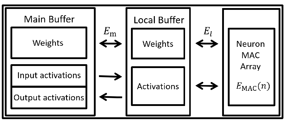
We consider a typical two dimensional processing chip for CNN as shown in Fig. 2 [4]. This chip has a parallel neuron array, MAC units, and two levels of memory: a main and a local buffer. A main buffer stores the current layers’ weights and activations, while a local buffer caches currently used weights and activations. From [13], we use the energy model of a MAC operation for levels of precision , where , , and is the maximum precision level. Here, a MAC operation includes the operation of a layer such as output calculation, batch normalization, activation, and weight update. Then, the energy consumption for accessing a local buffer can be modeled as , and the energy for accessing a main buffer is [4] .
The energy consumption of device for one iteration of local training is given by when bits are used for the precision level in the quantization. Then, is the sum of the computing energy , the access energy for fetching weights from the buffers , and the access energy for fetching activations from the buffers , as follows [13]:
| (9) |
where is the number of MAC operations, is the number of weights, and is the number of intermediate outputs throughout the network. For , in a QNN, batch normalization, activation function, gradient calculation, and weight update are done in full-precision to each output [11]. Once we fetch weights from a main to a local buffer, they can be reused in the local buffer afterward as shown in . In Fig. 2, a MAC unit fetches weights from a local buffer for computation. Since we are using a two dimensional MAC array of MAC units, they can share fetched weights with the same row and column, which has MAC units respectively. In addition, a MAC unit can fetch more weights due to the quantization with bits compared with when weights are represented in bits. Thus, we can reduce the access to a local buffer by the amount of . A similar process applies to since activations are fetched (stored) from (to) the main buffer.
II-C2 Transmission Model
We use OFDMA (OFDMA) to transmit a model update to the BS. The achievable rate of device is given by
| (10) |
where is the allocated bandwidth, is the channel gain between device and the BS, is the transmit power of each device, and is the power spectral density of white noise. After local training, device will transmit to the BS at given global iteration . Then, the transmission time for uploading is given by
| (11) |
Note that is quantized with bits of precision while is represented with bits. Then, the energy consumption for the uplink transmission is given by
| (12) |
In the following section, we formulate an energy minimizing problem based on the derived energy models.
III Proposed Approach for Energy-Efficient Federated QNN
We formulate an energy minimization problem while ensuring convergence under a target accuracy. A tradeoff exists between the energy consumption and the convergence rate with respect to . Hence, finding the optimal is important to balance the tradeoff and achieve the target accuracy. We propose a numerical method to solve this problem.
We aim to minimize the expected total energy consumption until convergence under the target accuracy as follows:
| (13a) | ||||
| s.t. | (13b) | |||
| (13c) | ||||
where is the number of local iterations, is the expectation of global loss function after global iteration, is the minimum value of , and is the target accuracy.
Since devices are randomly selected at each global iteration, we can derive the expectation of the objective function of (13a) as follows
| (14) |
To represent with respect to , we assume that the loss function is -smooth, -strongly convex and that the variance and the squared norm of the stochastic gradient are bounded by and for device , , respectively. Before we present the expression of , in the following lemma, we will first analyze the quantization error of the stochastic quantization in Sec. II.
Lemma 1.
For the stochastic quantization , a scalar value , and a vector , we have
| (15) | ||||
| (16) |
Proof.
From Lemma 1, we can see that our quantization scheme is unbiased as its expectation is zero. However, the quantization error can still increase for a large model. We next leverage the results of Lemma 1, [9], and[14] so as to derive with respect to in the following proposition.
Proposition 1.
For learning rate , we have
| (20) |
where is
| (21) |
Proof.
From Proposition 1, We let (20) be upper bounded by in (13c) as follows
| (22) |
We then take equality in (22) to obtain and approximate the problem as
| (23a) | ||||
| s.t. | (23b) | |||
Note that any optimal solution from problem (23a) can satisfy problem (13a) [15]. For any feasible from (22), we can always choose such that satisfies (13c).
Now, we relax as a continuous variable, which will be rounded back to an integer value. From (9), (12), and (21), we can observe that, as increases, and becomes larger while decreases. Hence, we can know that a local optimal may exist for minimizing . Since is differentiable with respect to in the given range, we can find by solving from Fermat’s Theorem [16]. Although it is difficult to derive analytically, we can obtain it numerically using a line search method. Hence, we can find a local optimal solution, which minimizes the total energy consumption under the given target accuracy.
IV Simulation Results
For our simulations, we uniformly deploy devices over a square area of size m m serviced by one BS at the center, and we assume a Rayleigh fading channel with a path loss exponent of 2. We also use MNIST dataset. Unless stated otherwise, we use mW, MHz, dBm, , , bits, , , , , , , and , [17]. For the computing model, we set pJ and as done in [13], and we assume that each device has the same architecture of the processing chip. All statistical results are averaged over independent runs

Figure 3 shows the total energy consumption of the FL system until convergence for varying levels of precision . In Fig. 3, we assume a QNN structure with two convolutional layers: 32 kernels of size with one padding and three of strides and 32 kernels of size with one padding and two of strides, each followed by max pooling. Then, we have one dense layer of 220 neurons and one fully-connected layer. In this setting, we have and . From this figure, we can see that the total energy consumption decreases and then increases with . This is because when is small, quantization error becomes large as shown in Lemma 1, which slows down the convergence rate in (20). However, as increases, the energy consumption for the local training and transmission also increases. Hence, a very small or very high may induce undesired large quantization error or unnecessary energy consumption due to a high level of precision. From this figure, we can see that can be optimal for minimizing energy consumption for our system.

Figure 4 shows the optimal level of precision when varying the number of local iterations . We use the same CNN architecture in Fig. 3. We can observe that increases with . This is because, as increases, the local models converge to the local optimal faster as SGD averages out the effect of quantization error [11]. Hence, a lower can be chosen by leveraging the increased to minimize the total energy consumption. We can observe that only is required at while we need at .

Figure 5 presents the optimal level of precision for varying model size . Note that equals to the number of model parameters . To scale the number of MAC operations for increasing accordingly, we set . From Fig. 5, we can see that increases with . From Lemma 1, the quantization error accumulates as increases. This directly affects the convergence rate in (20) resulting in both increased global iterations and the total energy consumption. Therefore, to mitigate the increasing quantization error from increasing , a larger level of precision may be chosen.

Figure 6 shows the total energy consumption and when varying a target accuracy . For these results, we use the same CNN architecture as Fig. 3. We can see that a higher accuracy level requires larger total energy consumption and more bits for data representation to mitigate the quantization error. In addition, the FL system needs a more number of global iterations to achieve from (22). As becomes looser, a lower can be chosen. From Fig. 6, we can see that an additional J energy is required to increase from 0.01 to while one additional bit of precision is needed.

Figure 7 compares the total energy consumption until convergence for varying the size of CNN models with the baseline that uses standard 32 bits for data representation. Case 1 is assumed to be CNN of two layers and have and . Case 2 and 3 are assumed to be CNN of five layers. They have and number of parameters and and number of MAC operations, respectively. Case 4 is 7 layers of CNN with and . Lastly, we assume Case 5 is 9 layers of CNN with and . The corresponding are 13, 14, 14 15, 15, respectively. We can see that our FL scheme is more effective for CNN models with a large model size. Note that Case 5 has 138.8 M weights while Case 1 has 25.6 M weights. In particular, for Case 5, we can reduce the total energy consumption up to 53 compared to the baseline.
V Conclusion
In this paper, we have studied the problem of energy-efficient quantized FL over wireless networks. We have presented the energy model for the quantized FL based on the physical structure of a processing chip and the convergence rate. Then, we have formulated an energy minimization problem that considers a level of precision in the quantized FL. To solve this problem, we have used a line search method. Simulation results have shown that our model requires much less energy than a standard FL model for convergence. The results particularly show significant improvements when the local models rely on large neural networks. In essence, this work provides the first holistic study of the tradeoff between energy, precision, and accuracy for FL over wireless networks.
References
- [1] T. Li, A. K. Sahu, A. Talwalkar, and V. Smith, “Federated learning: Challenges, methods, and future directions,” IEEE Signal Process. Mag., vol. 37, no. 3, pp. 50–60, May 2020.
- [2] H. B. McMahan, E. Moore, D. Ramage, S. Hampson, and B. A. Arcas, “Communication-efficient learning of deep networks from decentralized data,” arXiv preprint arXiv:1602.05629, 2017.
- [3] R. Schwartz, J. Dodge, N. A. Smith, and O. Etzioni, “Green AI,” arXiv preprint arXiv:1907.10597, 2019.
- [4] B. Moons, K. Goetschalckx, N. Van Berckelaer, and M. Verhelst, “Minimum energy quantized neural networks,” in Proc. of Asilomar Conf. on Signals, Systems, and Computers, Pacific Grove, CA, USA, Apr. 2017.
- [5] S. Savazzi, S. Kianoush, V. Rampa, and M. Bennis, “A framework for energy and carbon footprint analysis of distributed and federated edge learning,” arXiv preprint arXiv:2103.1034, 2021.
- [6] N. H. Tran, W. Bao, A. Zomaya, M. N. H. Nguyen, and C. S. Hong, “Federated learning over wireless networks: Optimization model design and analysis,” in Proc. of IEEE Conf. on Computer Commun., Paris, France, May 2019.
- [7] Z. Yang, M. Chen, W. Saad, C. S. Hong, and M. Shikh-Bahaei, “Energy efficient federated learning over wireless communication networks,” IEEE Trans. Wireless Commun., vol. 20, no. 3, pp. 1935–1949, Mar. 2021.
- [8] Q. Zeng, Y. Du, K. Huang, and K. K. Leung, “Energy-efficient resource management for federated edge learning with cpu-gpu heterogeneous computing,” IEEE Trans. Wireless Commun., 2021, to appear.
- [9] S. Zheng, C. Shen, and X. Chen, “Design and analysis of uplink and downlink communications for federated learning,” IEEE J. Sel. Areas Commun., vol. 39, no. 7, Jul. 2021.
- [10] Y. Yang, Z. Zhang, and Q. Yang, “Communication-efficient federated learning with binary neural networks,” IEEE J. Sel. Areas Commun., 2021, to appear.
- [11] I. Hubara, M. Courbariaux, D. Soudry, R. El-Yaniv, and Y. Bengio, “Quantized neural networks: Training neural networks with low precision weights and activations.” arXiv preprint arXiv:1609.07061, 2016.
- [12] S. Gupta, A. Agrawal, K. Gopalakrishnan, and P. Narayanan, “Deep learning with limited numerical precision,” in Proc. of International Conference on Machine Learning (ICML), Lille, France, Jul. 2015.
- [13] B. Moons, D. Bankman, and M. Verhelst, Embedded Deep Learning, Algorithms, Architectures and Circuits for Always-on Neural Network Processing. Springer, 2018.
- [14] X. Li, K. Huang, W. Yang, S. Wang, and Z. Zhang, “On the convergence of fedavg on non-iid data,” in Proc. of International Conference on Learning Representations (ICLR), May 2020.
- [15] B. Luo, X. Li, S. Wang, J. Huangy, and L. Tassiulas, “Cost-effective federated learning design,” in Proc. of IEEE Conf. on Computer Commun., Vancouver, BC, Canada, May 2021.
- [16] H. H. Bauschke, P. L. Combettes et al., Convex analysis and monotone operator theory in Hilbert spaces. Springer, 2011, vol. 408.
- [17] L. M. Nguyen, P. H. Nguyen, M. van Dijk, P. Richtarik, K. Scheinberg, and M. Takac, “Sgd and hogwild! convergence without the bounded gradients assumption,” in Proc. of International Conference on Machine Learning (ICML), Stockholm, Sweden, Jul. 2018.