Remarks on Fixed Point Assertions in Digital Topology, 5

A digital metric space [9] is a triple $(X,d,\kappa)$, where $(X,\kappa)$ is a digital image and $d$ is a metric on $X$. The metric is usually taken to be the Euclidean metric or some other $\ell_{p}$ metric. We are not convinced that the digital metric space is a notion worth developing. Typically, assertions in the literature do not make use of both $d$ and $\kappa$, so that “digital metric space” seems an artificial notion. E.g., for a discrete topological space $X$, all functions $f:X\to X$ are continuous, although on digital images, many functions $g:X\to X$ are not digitally continuous (digital continuity is defined in [2], generalizing an earlier definition [15]).

Figure 1 shows the definition appearing in [11] of a Kannan digital contraction.

Figure 2 shows a fixed point assertion for Kannan digital contractions in [11]. The “proof” of this assertion has errors discussed below.

• •

  In the fourth and fifth lines of the “proof” is the claim that

  $$\lambda[d(x_{n},x_{n-1})+d(x_{n-1},x_{n-2})]\leq 2\lambda d(x_{n},x_{n-1}).$$

  Since $\lambda>0$, this claim implies

  $$d(x_{n-1},x_{n-2})\leq d(x_{n},x_{n-1}),$$

  so if any $d(x_{n},x_{n-1})$ is positive, the sequence $\{x_{n}\}$ is not a Cauchy sequence, contrary to a claim that appears later in the argument.

• •

  Towards the end of the existence argument, the authors claim that a Kannan digital contraction is digitally continuous. This assumption is contradicted by Example 4.1 of [6].

In light of these errors, we must conclude that the assertion of Figure 2 is unproven.

This example is shown in Figure 3. One sees easily the following.

• •

  $d(0,1)=d(0,2)=0$, so $d$, contrary to the claim, is not a metric.

• •

  $T(1)=1/2\not\in X$.

Figure 4 shows an assertion of a fixed point result on p. 10770 of [11].

Note “And let $f$ satisfies” should be “and let $T$ satisfy”.

More importantly: In the argument offered as proof of this assertion, the authors let $x_{0}\in X$, and, inductively,

They claim that by using the statements marked (i) and (ii) in Figure 4, it follows that

which, despite the authors’ claim, does not show that the sequence $\{a_{n}\}$ is decreasing. However, what correctly follows from the statements marked (i) and (ii) in Figure 4 is

From this we see that $a_{n+1}<a_{n}$, so the sequence $\{a_{n}\}$ is decreasing and bounded below by 0, hence tends to a limit $a\geq 0$.

The authors then claim that if $a>0$ then $a_{n+1}\leq Y(a_{n})$. However, what we showed in (2) does not support this conclusion, which is not justified in any obvious way. Since the authors wish to contradict the hypothesis that $a>0$ in order to derive that the sequence $\{x_{n}\}$ is a Cauchy sequence, we must regard the assertion shown in Figure 4 as unproven.

A Zamfirescu digital contraction is defined in Figure 5. This notion is used in [11, 14], and will be discussed in the current section and in section 6.

Figure 6 shows an assertion found on p. 10770 of [11].

The argument offered as “proof” of this assertion considers cases. For an arbitrary $x_{0}\in X$, a sequence is inductively defined via $x_{n+1}=T(x_{n})$. For convenience, let us define

The argument considers several cases.

• •

  Case 1 says if $d(x_{n+1},x_{n})=M(x_{n+1},x_{n})$ then, by implied induction,

  $$d(x_{n+1},x_{n})\leq\lambda^{n}d(x_{1},x_{0}).$$

  But this argument is based on the unproven assumption that this is also the case for all indices $i<n$; i.e., that $d(x_{i+1},x_{i})=M(x_{i+1},x_{i})$.

• •

  Case 2 says if

  $$\frac{d(x_{n+1},Tx_{n+1})+d(x_{n},Tx_{n})}{2}=$$

  $$\max\left\{\begin{array}[]{l}d(x_{n+1},x_{n}),\frac{d(x_{n+1},Tx_{n+1})+d(x_{n},Tx_{n})}{2},\\ \\ \frac{d(x_{n+1},Tx_{n})+d(x_{n},Tx_{n_{1}})}{2}\end{array}\right\},$$

  then

  $$d(x_{n+1},x_{n})=d(Tx_{n},Tx_{n-1})\leq\lambda\frac{d(x_{n},x_{n-1})+d(x_{n-1},x_{n-2})}{2}\leq$$

  $$\lambda d(x_{n},x_{n-1}).$$

  But in order for the second inequality in this chain to be true, we would need $d(x_{n-1},x_{n-2})\leq d(x_{n},x_{n-1})$, and no reason is given to believe the latter.

• •

  Case 3 says that if $\frac{d(x_{n+1},Tx_{n})+d(x_{n},Tx_{n+1})}{2}=M(x_{n+1},x_{n})$ then

  $$d(x_{n+1},x_{n})=d(Tx_{n},Tx_{n-1})\leq\lambda\frac{d(x_{n},x_{n-2})+d(x_{n-1},x_{n-1})}{2}.$$

  The correct upper bound, according to the definition shown in Figure 5, is

  $$\lambda\frac{d(x_{n+1},Tx_{n})+d(x_{n},Tx_{n+1})}{2}=\lambda\frac{d(x_{n+1},x_{n+1})+d(x_{n},x_{n+2})}{2}=$$

  $$\lambda\frac{d(x_{n},x_{n+2})}{2}.$$

  Further, the conclusion reached by the authors for this case, that the distances $d(x_{n+1},x_{n})$ are bounded above by an expression that tends to 0 as $n\to\infty$, depends on the unproven hypothesis that an analog of this case holds for all indices $i<n$.

Thus all three cases considered by the authors are handled incorrectly. We must conclude that the assertion of Figure 6 is unproven.

Figure 7 shows the definition appearing in [11] of a Rhoades digital contraction. The paper [11] claims the fixed point result shown in Figure 8 for such functions. The argument offered in “proof” of this assertion has errors that are discussed below.

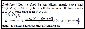
For convenience, let

The authors’ argument considers cases corresponding to which of the embraced expressions above gives the value of $M(x_{n+1},x_{n})$. In each case, the authors assume without proof that the same case is valid for $M(x_{i+1},x_{i})$, for all indices $i<n$.

Additional errors:

• •

  In case 2, the inequality

  $$d(Tx_{n},Tx_{n-1})\leq\lambda\frac{d(x_{n},x_{n-1})+d(x_{n-1},x_{n-2})}{2}$$

  should be, according to Figure 7,

  $$d(x_{n},x_{n+1})=d(Tx_{n},Tx_{n-1})\leq\lambda\frac{d(x_{n},Tx_{n})+d(x_{n+1},Tx_{n-1})}{2}$$

  $$=\lambda\frac{d(x_{n},x_{n+1})+d(x_{n+1},x_{n})}{2}=\lambda d(x_{n},x_{n+1}).$$

  Note this implies

  $$x_{n}=x_{n+1},$$

  (3)

  which would imply the existence of a fixed point. Also, the authors claim that

  $$\lambda\frac{d(x_{n},x_{n-1})+d(x_{n-1},x_{n-2})}{2}\leq\lambda d(x_{n},x_{n-1}),$$

  which is equivalent to

  $$d(x_{n-1},x_{n-2})\leq d(x_{n},x_{n-1}).$$

  No reason is given in support of the latter; further, it undermines the later claim that $\{x_{n}\}$ is a Cauchy sequence, since the authors did not deduce (3).

• •

  In case 3, it is claimed that

  $$\lambda d(x_{n},Tx_{n-1})\leq\lambda d(x_{n},x_{n-1}).$$

  This should be corrected to

  $$\lambda d(x_{n},Tx_{n-1})=\lambda d(x_{n},x_{n})=0,$$

  which would guarantee a fixed point.

• •

  In case 4, we see the claim

  $$d(x_{n-1},Tx_{n})=d(x_{n-1},x_{n-1})=0.$$

  This should be corrected to

  $$d(x_{n-1},Tx_{n})=d(x_{n-1},x_{n+1}).$$

In view of these errors, we must regard the assertion shown in Figure 8 as unproven.

The assertion stated as Theorem 3.1 in [1] is shown in Figure 9. In this section, we show the assertion is false except in a trivial case.

Note if $d$ is any $\ell_{p}$ metric (including the usual Euclidean metric) then the requirements of closed subsets of $X$ are automatically satisfied, since $(X,d)$ is a discrete space.

In Figure 10, we see the assertion presented as Example 3.1 of [1].

Note the following.

• •

  If “$X=[4,40]$” is meant to mean the real interval from 4 to 40, then $X$ is not a digital image, as all coordinates of members of a digital image must be integers. Perhaps $X$ is meant to be the digital interval $[4,40]_{{\mathbb{Z}}}=[4,40]\cap{\mathbb{Z}}$.

• •

  The function $G$ is not defined on all of $[4,40]_{{\mathbb{Z}}}$, appears to be doubly defined for some values of $x$, (notice the incomplete inequality at the end of the 3rd line) and is not restricted to integer values.

• •

  The function $H$ is not defined on all of $[4,40]_{{\mathbb{Z}}}$ and is doubly defined for $x\in\{13,14\}$.

• •

  The function $Q$ is not defined for $x\in\{9,10,11,12\}$, and is doubly defined for $x\in\{14,15\}$.

• •

  The “above theorem” referenced in the last sentence of Figure 10 is the assertion discredited by our Theorem 4.2, which shows that $P=Q=G=H$. Clearly, the assertion shown in Figure 10 fails to satisfy the latter.

Thus, Example 3.1 of [1] is not useful.

The assertion presented as Corollary 3.2 of [1] is presented in Figure 11. Notice that “weakly mappings” is an undefined phrase. No proof is given in [1] for this assertion, and it is not clear how the assertion might follow from previous assertions of the paper (which, as we have seen above, are also flawed).

Perhaps “weakly mappings” is intended to be “weakly compatible mappings”. At any rate, by labeling this assertion as a Corollary, the authors suggest that it follows from the paper’s flawed “Theorem” 3.1.

The assertion presented as “Corollary” 3.2 of [1] must be regarded as undefined and unproven.

References

- [1] S.K. Barve, Q.A. Kabir, and R.D. Daheriya, Unique common fixed point theorem for weakly compatible mappings in digital metric space, International Journal of Scientific Research and Reviews 8(1) (2019), 2114-2121
- [2] L. Boxer, A classical construction for the digital fundamental group, Journal of Mathematical Imaging and Vision 10 (1999), 51-62.
- [3] L. Boxer, Remarks on Fixed Point Assertions in Digital Topology, 2, Applied General Topology 20, (1) (2019), 155-175.
- [4] L. Boxer, Remarks on Fixed Point Assertions in Digital Topology, 3, Applied General Topology 20 (2) (2019), 349-361.
- [5] L. Boxer, Remarks on Fixed Point Assertions in Digital Topology, 4, Applied General Topology 21 (2) (2020), 265 - 284
- [6] L. Boxer and P.C. Staecker, Remarks on fixed point assertions in digital topology, Applied General Topology 20 (1) (2019), 135-153.
- [7] C. Chauhan, J. Singhal, S. Shrivastava, Q.A. Kabir, and P.K. Jha, Digital topology with fixed point, Materials Today: Proceedings 47 (2021) 7167-7169
- [8] S. Dalal, Common fixed point results for weakly compatible map in digital metric spaces, Scholars Journal of Physics, Mathematics and Statistics 4 (4) (2017), 196-201.
- [9] O. Ege and I. Karaca, Digital homotopy fixed point theory, Comptes Rendus Mathematique 353 (11) (2015), 1029-1033.
- [10] K. Jyoti and A. Rani, Fixed point theorems for - - -expansive type mappings in digital metric spaces, Asian Journal of Mathematics and Computer Research 24 (2) (2018), 56-66.
- [11] K. Jyoti and A. Rani, Fixed point theorems with digital contractions, International Journal of Current Advanced Research 7 (3(E)) (2018), 10768-10772
- [12] A. Mishra, P.K. Tripathi, A.K. Agrawal, and D.R. Joshi, A contraction mapping method in digital image processing, International Journal of Recent Technology and Engineering 8 (4S5) (2019), 193 - 196
- [13] L.N. Mishra, K. Jyoti, A. Rani, and Vandana, Fixed point theorems with digital contractions image processing, Nonlinear Science Letters A 9 (2) (2018), 104 - 115
- [14] K. Rana and A. Garg, Various contraction conditions in digital metric spaces, Advances in Mathematics: Scientific Journal 9 (2020), no.8, 5433-5441
- [15] A. Rosenfeld, ‘Continuous’ functions on digital pictures, Pattern Recognition Letters 4, pp. 177-184, 1986.